Thermodynamics of Adiabatically Loaded Cold Bosons in the Mott Insulating Phase of One-Dimensional Optical Lattices

Abstract

In this work we give a consistent picture of the thermodynamic properties of bosons in the Mott insulating phase when loaded adiabatically into one-dimensional optical lattices. We find a crucial dependence of the temperature in the optical lattice on the doping level of the Mott insulator. In the undoped case, the temperature is of the order of the large onsite Hubbard interaction. In contrast, at a finite doping level the temperature jumps almost immediately to the order of the small hopping parameter. These two situations are investigated on the one hand by considering limiting cases like the atomic limit and the case of free fermions. On the other hand, they are examined using a quasi-particle conserving continuous unitary transformation extended by an approximate thermodynamics for hardcore particles.

I Introduction

The design of tunable quantum systems with strong correlations has attracted much interest due to the fast experimental developments in the field of ultracold atoms loaded in optical lattices. It has become possible in experiment to vary the dimension of the optical lattices and the particle statistics of the involved ultracold atoms Jaksch et al. (1998); Greiner et al. (2002); Stöferle et al. (2004); Paredes et al. (2004); Kinoshita et al. (2004); Köhl et al. (2005). This opens the road to study fascinating quantum many-body effects like superfluidity in artificially created and thus tunable structures.

In order to investigate these quantum effects the temperature of the ultracold atoms in the optical lattice has to be small in units of typical model parameters. Experimentally it is an open problem to measure this temperature. We have addressed this question in a recent work Reischl et al. (2005) theoretically by analyzing spectroscopic experiments on bosons in one-dimensional optical lattices Stöferle et al. (2004). We found that the temperature in the Mott insulating phase is surprisingly large, namely of the order of the onsite Hubbard interaction $U$. In an analogous experiment the so-called Tonks-Girardeau regime (TG) was investigated Paredes et al. (2004). From this experiment, a rather small temperature of the order of the hopping parameter $t$ has been deduced.

In the present work we provide a consistent thermodynamic picture of both experiments. The large difference in temperature can be understood solely from entropy considerations. In the undoped Mott insulator the groundstate is unique and does not carry any entropy. It is separated from excited states by an energy gap which is determined by the interaction $U$. The entropy increases appreciably only at temperatures which are of the order of the gap. In a doped Mott insulator describing the TG regime the low-lying states produce a finite entropy and the temperature of the bosons is much smaller.

The paper is organized as follows. We will first introduce the model and our notation. In Sect. III we will study several analytically solvable limits. First, we calculate the entropy of non-interacting bosons in a trap relevant for the cold atoms before loading into the optical lattice. Then we consider the atomic limit and the limit of non-interacting fermions which corresponds to the TG case. In Sect. IV a continuous unitary transformation (CUT) is used to study the Mott insulating phase of the Bose-Hubbard model at zero temperature. The results are extended to finite temperatures by an approximate formalism appropriate for hardcore particles. We first test the reliability of this approximation by comparison to exact results in the case of non-interacting fermions. Then the thermodynamic properties of the doped and undoped Mott insulating phase of the one-dimensional Bose-Hubbard model are studied. The conclusions will summarize the essence of the paper. In the last section, we propose an experimental procedure to reach very low temperatures also for the Mott insulating phase.

II Model

Bosonic atoms in an optical lattice are described by the Bose-Hubbard model Jaksch et al. (1998). The Hamiltonian reads

$$H = tH_{t}+UH_{U}+\mu H_{\mu}$$

$$= -t\sum\limits_{i}(b^{\dagger}_{i}b^{\phantom{\dagger}}_{i+1}+b^{\dagger}_{i+1}b^{\phantom{\dagger}}_{i})$$

$$+ (U/2)\sum_{i}\hat{n}_{i}(\hat{n}_{i}-1)-\mu\sum_{i}\hat{n}_{i}$$

where the first term is the kinetic part $tH_{t}$ and the second term the repulsive interaction $UH_{U}$ with $U>0$. The last term accounts for a chemical potential $\mu$. The bosonic annihilation (creation) operators are denoted by $b^{(\dagger)}_{i}$, the number of bosons by $\hat{n}_{i}=b^{\dagger}_{i}b^{\phantom{\dagger}}_{i}$. The average number of bosons is $n=\langle\hat{n}_{i}\rangle=N/L$ where $N$ is the total number of bosons and $L$ the total number of wells in the optical lattice. In the spirit of the tight-binding description we will call the wells henceforth ‘sites’. On the same site, the bosons repel each other with interaction strength $U$.

In the limit $t/U\to 0$, a site with $n$ bosons contributes the energy $E(n)=(U/2)n(n-1)$. A deviation from uniform filling costs the energy $E(n+1)+E(n-1)-2E(n)=U$. Note that this excess energy results from the constant curvature of the parabola $\propto n^{2}$. Thus it is independent of $n$. For large $U$ and integer filling $n$ it is energetically favorable to distribute the bosons uniformly and to put just $n$ bosons on each site. The system is in an insulating state with an energy gap of the order of $U$.

In the opposite limit of large $t/U$ the bosons form a superfluid condensate for low enough temperatures.

We will not address the inhomogeneity that is present in the experimentally realized traps, i.e., we treat the system as translationally invariant though there is the slowly varying external trap potential. This approach makes quantitative computations much easier and it is backed by the recent finding that the inhomogeneous system acts essentially like two (or several) independent systems of different average number of bosons Batrouni et al. (2005).

Among the extensive literature on the bosonic Hubbard model there are mean-field treatments, e.g. Refs. Jaksch et al., 1998; Krauth et al., 1992; Sheshadri et al., 1993; van Oosten et al., 2001, other analytical investigations, e.g. Refs. Fisher et al., 1989; Elstner and Monien, 1999; Krauth, 1991; Dickerscheid et al., 2003, and numerical treatments, e.g. Refs. Pai et al., 1996; Kashurnikov and Svistunov, 1996; Kühner and Monien, 1998; Kühner et al., 2000; Reischl et al., 2005. The phase diagram in the $t$-$\mu$-plane consists of a series of lobes. The lobes of the Mott insulating phases correspond to an integer filling per site. The present paper is only concerned with the first lobe of the phase diagram where $n=1$.

III Limiting Cases

Three limiting cases are investigated in order to understand the basic entropy properties of the cold atoms before and after adiabatic loading into the optical lattice. First, we calculate the entropy of non-interacting bosons in a trap. This entropy is present before turning on the optical lattice. It can be viewed as a function of the superfluid fraction. The same entropy has to be realized in the optical lattice once it has been turned on in an adiabatic fashion. Hence the adiabaticity of the loading determines the temperature of the bosons in the optical lattice Blakie and Porto (2004). We calculate the entropy as a function of the microscopic model parameters and of the doping in the atomic limit, $t/U=0$ and in the limit of infinite $U$, the so-called TG regime. In one dimension Jordan and Wigner (1928); Tonks (2002); Girardeau (1960), a Jordan-Wigner mapping to non-interacting fermions is appropriate.

III.1 Free Bosons

The formula for the entropy of free bosons in a wide harmonic trap is derived. The Hamiltonian of the harmonic oscillator in $d$ dimensions reads ($\hbar=1$)

$$H=\omega_{0}\sum_{j=1}^{d}a^{\dagger}_{j}a^{\phantom{\dagger}}_{j}.$$ (2)

Many bosons loaded in the harmonic trap are considered. The energy $\omega_{0}$ is small. Therefore, sums over multiples of $\omega_{0}$ can be rewritten as integrals. The groundstate is macroscopically occupied with a fraction

$$f_{0}=N_{0}/N$$ (3)

where $N$ is the total number of bosons and $N_{0}$ their number in the condensate. With the density of states $D(\omega)$ and the boson occupation $n_{\text{B}}(\omega)=1/(e^{\beta\omega}-1)$ one has

$$N = N_{0}+\sum_{m=1}^{\infty}n_{\text{B}}(m\omega_{0})D(m\omega_{0})$$ (4a)

$$= Nf_{0}+\int_{0}^{\infty}n_{\text{B}}(\omega)D(\omega)d\omega\ .$$ (4b)

The density of states $D(\omega)$ counts the number of states in a given energy interval. Let us consider intervals of length $\omega_{0}$ centered around the energies $m\omega_{0}$, where $m$ is a non-negative integer. We consider the number of ways in which the energy $\omega=m\omega_{0}$ can be realized. One has to distribute $m$ indistinguishable energy quanta over $d$ oscillators. The number of possibilities is

$$D(m\omega_{0})\omega_{0}=\binom{m+d-1}{d-1}\ .$$ (5)

Using $m=\omega/\omega_{0}$, the leading power in $\omega$ reads

$$D(\omega)=\frac{1}{\omega_{0}(d-1)!}\left(\frac{\omega}{\omega_{0}}\right)^{d-1}\ .$$ (6)

Only the leading order in $m=\omega/\omega_{0}$ is retained because a wide trap potential is considered which implies a small oscillator frequency $\omega_{0}$.

Specializing to our case of interest, a three-dimensional trap ($d=3$), Eq. 4b becomes

$$N=Nf_{0}+\frac{T^{3}}{2}\int_{0}^{\infty}\frac{x^{2}}{e^{x}-1}dx=Nf_{0}+T^{3}\zeta(3),$$ (7)

where $x=\beta\omega$ and $\zeta(z)$ is the Riemann $\zeta$-function. Furthermore, we need the total entropy. The entropy of a single bosonic level $\epsilon$ reads ($k_{\rm B}=1$)

$$S(\epsilon)=-\ln(1-e^{-\beta\epsilon})+\beta\epsilon n_{\text{B}}(\epsilon)\ .$$ (8)

The total entropy is given by

$$S^{\text{tot}}=\int_{0}^{\infty}S(\epsilon)D(\epsilon)d\epsilon=\frac{2\pi^{4}}{45}\left(\frac{T}{\omega_{0}}\right)^{3}\ .$$ (9)

The condensate at zero energy does not contribute to the entropy because it represents a single, pure quantum state. Combining Eqs. (7) and (9) leads to

$$S/N=(1-f_{0})\frac{2\pi^{4}}{45\zeta(3)}\approx 3.60(1-f_{0})\quad.$$ (10)

This relation between entropy and superfluid fraction will serve in the following as the initial entropy of the cold atoms before turning on the optical lattice.

III.2 Atomic Limit

In this part, we calculate the entropy as a function of temperature and doping in the atomic limit, namely $t/U=0$. Then, all excitation processes are completely local. For simplicity, we restrict the local Hilbert space to the state with occupation one and the two energetically adjacent states with occupation zero and two. The energy to create a site with two bosons is $U$. All states with an even larger number of bosons have a higher energy and are therefore not important for the entropy in the temperature range considered here.

The Gibbs energy of a single site is given by

$$g=-T\ln\left[1+e^{\beta\mu}+e^{-\beta(U-2\mu)}\right]\ ,$$ (11)

where the terms in the argument of the logarithm refer to the empty, the singly occupied and the doubly occupied site. Introducing the doping $\delta:=n-1$ and using $\left.\partial_{\mu}g\right|_{T}=-n=-(1+\delta)$ we arrive at the following expression for the chemical potential at given doping $\delta$

$$\mu=\frac{1}{\beta}\ln\left[\frac{\delta e^{\beta U}}{2(1-\delta)}\left(1-\sqrt{1+\left(4/\delta^{2}-4\right)e^{-\beta U}}\right)\right].$$ (12)

The entropy per particle is calculated as the derivative of the Gibbs energy with respect to temperature $S/N=S/(nL)=-\left.\partial_{T}f\right|_{\mu}$. In Fig. 1 the entropy is shown for $n\in\{1;0.99;0.95;0.9;0.8\}$. Additionally, the entropy for free bosons with a superfluid fraction $f_{0}=\{0.95;0.9;0.8\}$ according to Eq. 10 is given. All curves display an almost constant plateau at small temperatures $T/U<0.1$, an uprise at about $T/U\sim 0.3$ and a saturation for large temperatures.

Figure 1: Entropy per particle as a function of temperature in the atomic limit $t/U=0$ for various values of doping. The entropy per particle of the three-dimensional harmonic oscillator for condensate fractions $f_{0}=0.95;0.9;0.8$ is included as black horizontal lines.

Supposing that the bosons are loaded adiabatically, three different regimes can be identified for fixed $f_{0}$. In the following, the experimentally relevant value $f_{0}=0.9$ is discussed. At zero doping, the temperature is approximately $U/6$, i.e., of the same order as deduced by analysing recent spectroscopic experiments Reischl et al. (2005); Stöferle et al. (2004). This seemingly large value for the temperature is needed because the groundstate of the Mott insulating phase at zero doping is separated by a large gap from the first excited states. The entropy has to be produced by the excited states which have an energy of the order $U$.

A small amount of doping leaves this temperature almost unchanged. But the system develops a finite entropy at zero (and small) temperatures. The reason for this is the degeneracy of the groundstate coming from the different possibilities to distribute $N$ bosons over $L$ lattice sites. The entropy at intermediate values of the temperature is only changed slightly. The temperature realized in the optical lattice is changed abruptly when the zero temperature entropy reaches the entropy value of the free bosons. Then the temperature immediately jumps to zero. Physically this corresponds to the situation where the whole entropy can be produced by the groundstate degeneracy of the doped Mott insulator. Thereby the temperature is reduced to the scale $t$ which is zero in the atomic limit. This is the mechanism which is most probably observed in the experiment in Ref. Paredes et al., 2004. It is more closely examined in the next part.

In the third temperature regime, the entropy of the free bosons is smaller than the entropy of the adiabatically loaded bosons at any temperature. This means that an adiabatic loading of the bosons into the optical lattice is not possible. Instead, a non-ergodic mixture will be realized. We emphasize, however, that this feature results from the macroscopic ground-state degeneracy in the atomic limit which represents an extreme and idealized situation.

III.3 Tonks-Girardeau Regime

The experiment performed in Ref. Paredes et al., 2004 probes the so-called Tonks-Girardeau (TG) regime Jordan and Wigner (1928); Girardeau (1960); Tonks (2002); Lieb and Liniger (1963). This is the limit of large $U$. Only empty and singly occupied sites are present and the problem can be mapped in one dimension onto fermions without interaction if we consider nearest-neighbor hopping only. If we relax the condition of nearest-neighbor hopping the mapping to fermions can still be done but the resulting system is not without interaction. Hence we focus here on nearest-neighbor hopping so that we have a benchmark system which is simple to analyze.

In order to know which temperature is realized after adiabatic loading in the TG regime one needs to know the entropy of the non-interacting fermion gas. In one dimension the dispersion of tight-binding fermions with hopping $-t$ reads

$$\epsilon(k)=-2t\cos(k).$$ (13)

Figure 2: Entropy of non-interacting tight binding fermions corresponding to the TG regime for various fillings. The entropy per particle of the three-dimensional harmonic oscillator for condensate fraction $f_{0}=0.95;0.9;0.8$ is included as black horizontal lines.

The Gibbs energy per site is ($k_{\rm B}=1$)

$$g = \frac{G}{L}=-\frac{T}{L}\sum_{k}\ln(1+e^{-\beta\epsilon(k)})$$ (14)

$$= -\frac{T}{2\pi}\int_{-\pi}^{\pi}\ln(1+e^{-\beta\epsilon(k)})dk$$ (15)

where $L$ is the number of sites. The entropy per particle is calculated as

$$\frac{S}{N} = \frac{1}{n}\frac{S}{L}=-\frac{1}{n}\left.\frac{\partial g}{\partial T}\right|_{\mu}$$

$$= \frac{k_{b}}{\pi}\int_{-\pi}^{\pi}\left(\ln(1+e^{-\beta\epsilon(k)})+\frac{\epsilon(k)}{T(1+e^{-\beta\epsilon(k)})}\right)dk\quad.$$

In the limit of high temperatures the entropy per site is

$${S}/{L}=-n\log(n)-(1-n)\log(1-n)$$ (17)

which is just the entropy of one state with occupation probability $n$. The entropy per particle is accordingly

$${S}/{N}=-\log(n)+(1-{n}^{-1})\log(1-n).$$ (18)

Figure 2 shows the entropy per particle versus $T/t$ in the TG regime for fillings $n\in\{0.5,0.6,0.7,0.8,0.9\}$. After a steep increase the entropy reaches its saturation value of $-\log(n)+(1-{n}^{-1})\log(1-n)$. Filling $n=0.5$ shows the largest saturation value. If the filling is increased further the saturation value decreases. Note that the $S/L$ is particle-hole symmetric, i.e., it does not matter whether we consider the filling of fermions $n$ or the filling of holes $1-n$.

Additionally, the entropy per particle of the three-dimensional harmonic trap is plotted for condensate fractions $f_{0}=0.95;0.9;0.8$ as horizontal lines. This allows to determine the temperature that results for these condensate fractions after loading into the optical lattice in the TG regime. For half filling $n=0.5$, the temperatures are $T/t=0.17;0.32;0.61$ for $f_{0}=0.95;0.9;0.8$. Also temperatures of multiples of the hopping parameter are possible, e.g., for $f_{0}=0.838$ and $n=0.8$ the temperature is $T/t=2$. Again, the temperatures are of the size of the microscopic system parameter $t$. This agrees well with the temperatures estimated in Ref. Paredes et al., 2004. There, the temperature has been determined from the measured momentum profiles.

For higher filling the entropy saturates at a lower value. For filling $n=0.8$ it does not rise up to the value of the harmonic trap for $f_{0}=0.8$. Thus in a process of adiabatic loading one cannot achieve a filling of $n=0.8$ when starting with a condensate fraction of $f_{0}=0.8$. Within the TG regime, even the highest temperatures are not sufficient to reach the necessary entropy. In practice this means that a system starting from too high an initial entropy will not end up in the TG regime. Doubly occupied sites will occur corresponding to temperatures of the order of the corresponding gap. This means that the description as non-interacting gas of fermions will no longer hold.

IV Continuous Unitary Transformation

After having discussed the atomic limit and the case of free fermions, we study the Bose-Hubbard Hamiltonian at finite $t/U$ by means of a particle conserving CUT at zero temperature Reischl et al. (2005). We reformulate the model in terms of new quasi-particles above the reference state with one boson per site. These particles obey hardcore statistics. Aspects of the method will be presented in the next subsection. The focus is again laid on thermodynamic, mainly entropy, considerations. We adapt a formalism introduced for spin ladders Troyer et al. (1994) to approximate the hardcore statistics to obtain results at finite temperature Reischl et al. (2005). In subsection IV.2 this formalism is introduced for the case of the Bose-Hubbard Hamiltonian. In particular, we check the reliability of the approximate hardcore statistics by comparison to the results of non-interacting fermions in the TG regime. At the end of this part, we present results for the entropy and the temperature of the undoped and doped Mott insulating phase for finite $t/U$.

IV.1 Method

In this part some technical aspects concerning the CUT are presented. For the general method we refer the interested reader to Refs. Knetter and Uhrig, 2000; Knetter et al., 2003; Reischl et al., 2004, 2005. To set up the CUT calculation the reference state has to be fixed. For $t/U\to 0$ and filling $n=1$ the groundstate of Eq. II is the product state of precisely one boson per site

$$|\text{ref}\rangle=|1\rangle_{1}\otimes|1\rangle_{2}\ldots\otimes|1\rangle_{N},$$ (19)

where $|n\rangle_{i}$ denotes the local state at site $i$ with $n$ bosons. We take $|\text{ref}\rangle$ as the reference state. For finite $t/U$ the kinetic part $tH_{t}$ will cause fluctuations around the reference state. Deviations from $|\text{ref}\rangle$ are considered to be elementary excitations. Each site can be occupied by an infinite number of bosons. The local Hilbert space has infinite dimensions. Therefore, there are also infinitely many linear independent local operators on this space. To set up a real space CUT, it is convenient to truncate the otherwise proliferating number of terms Reischl et al. (2004, 2005). In the present work, the local bosonic Hilbert space is truncated to four states. Numerical studies using density-matrix renormalization group have shown that this does not change the relevant physics Pai et al. (1996); Kashurnikov and Svistunov (1996); Kühner and Monien (1998). The CUT gives reliable results in a wide parameter regime up to $t/U\approx 0.2$, see Ref. Reischl et al., 2005. Since the calculation is restricted to four local states including the reference state there are three local creation operators. Applied to the reference state $|\text{ref}\rangle_{i}=|1\rangle_{i}$ they create local excitations. A hole at site $i$ is created by $h^{\dagger}_{i}|1\rangle_{i}=|0\rangle_{i}$, a particle by $p^{\dagger}_{i}|1\rangle_{i}=|2\rangle_{i}$, and $d^{\dagger}_{i}|1\rangle_{i}=|3\rangle_{i}$ induces another kind of particle at site $i$. The particle created by $d^{\dagger}_{i}$ corresponds to a local occupation of a site by three bosons which is treated as an independent quasi-particle. The operators $h$, $p$ and $d$ obey the commutation relations for hardcore bosons. The local bosonic operator $b^{\dagger}_{i}$ is thus represented by the $4\times 4$ matrix

$$b^{\dagger}_{i}=h^{\phantom{\dagger}}_{i}+\sqrt{2}p^{\dagger}_{i}+\sqrt{3}d^{\dagger}_{i}p^{\phantom{\dagger}}_{i}\to\left(\begin{array}[]{cccc}0&0&0&0\\ 1&0&0&0\\ 0&\sqrt{2}&0&0\\ 0&0&\sqrt{3}&0\\ \end{array}\right)_{\text{\large\it i}}\ ,$$ (20)

which acts on the vector of the coefficients of $\{|0\rangle,|1\rangle,|2\rangle,|3\rangle\}$. The CUT is implemented using this presentation of the Hamiltonian with finite local matrices Reischl et al. (2004). The Hamiltonian Eq. II conserves the number of bosons. But if it is rewritten in terms of $h,p,d$ it does not conserve the number of these newly introduced particles. For example, the application of $H_{t}$ to $|\text{ref}\rangle$ generates a particle-hole pair. To eliminate the terms that change the eigenvalue of $H_{U}$ an infinitesimal generator of the CUT is chosen as

$$\eta_{i,j}(l)={\rm sgn}\left(q_{i}-q_{j}\right)H_{i,j}(l)$$ (21)

in an eigenbasis of $H_{U}$; $q_{i}$ is the corresponding eigenvalue of $H_{U}$, see Ref. Knetter and Uhrig, 2000. The choice of this generator leads to an effective Hamiltonian commuting with $H_{U}$ which implies that the processes changing the number of quasiparticles are eliminated. For the bosonic Hubbard model a complete elimination cannot be achieved due to the occurrence of life time effects Reischl et al. (2005). But this effect is of minor importance in the parameter regime under study.

The bottom line is that the CUT maps the complicated elementary excitations of the bosonic Mott insulator onto hardcore particles. The corresponding annihilation (creation) operators are $p^{(\dagger)}$, $h^{(\dagger)}$, and $d^{(\dagger)}$.

IV.2 Finite Temperatures

In order to discuss thermodynamic properties of the Bose-Hubbard model we have to extend the calculation to finite temperatures. The CUT yields an effective Hamiltonian. The particles involved obey hardcore commutation relations. The statistics of hardcore particles, however, is complicated and thus a direct evaluation of the partition function is not easily tractable. In order to obtain results at finite temperature we will adapt the calculation in Ref. Troyer et al., 1994 for hardcore triplet excitations, called triplons, to our present purposes.

The explicit derivation of the approximate Gibbs energy for hardcore bosons is presented in Appendix A. The resulting Gibbs energy per particle reads

$$g=-(T/L)\ln\tilde{Z}=-T\ln(1+z^{p}+z^{h}),$$ (22)

where we use partition functions for the individual particles defined in Eq. (30).

IV.3 Test of the Approximate Thermodynamics

We check the validity of the approximate thermodynamics. The results for the TG regime from the previous section, Sect. III.3, are used as a benchmark. In particular, the quality of the approximate statistics for low temperatures and fillings $n\neq 1$ is addressed.

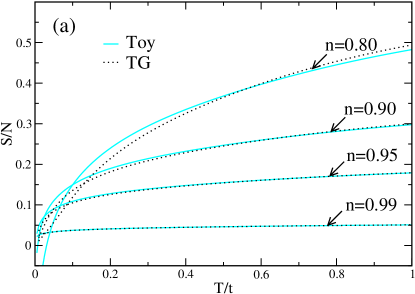
Figure 3: Comparison of entropies per particle at small temperatures calculated for the TG regime. (a) (color online) Entropy of free fermions is shown as dotted black curves. Results from the toy model calculation in gray (cyan). For fillings close to $n=1$ the entropies show good agreement. But deviations increase with increasing doping and for decreasing temperature. (b) Relative deviation $\Delta_{S}=(S_{\text{Toy}}-S_{\text{TG}})/S_{\text{TG}}$ of the entropy of the toy-model from the TG result.

For this purpose, we introduce a toy model which corresponds to the TG regime. The CUT calculation deals with the situation found for the bosonic Hubbard model for filling $n=1$ and for values $t/U$ in the Mott insulating phase. Above the groundstate of singly occupied sites there exist particle- and hole-like excitations. The toy model includes only the hole-like particles. Its Gibbs energy in Eq. 22 simplifies accordingly (cf. Appendix A)

$$g_{\text{toy}}=-T\ln(1+z^{h})\ .$$ (23)

The dispersion contains only a single cosine-term

$$\omega^{h}(k)=-2t\cos(k)$$ (24)

corresponding to hardcore bosons with nearest-neighbor hopping only. With these definitions the toy model describes the TG regime.

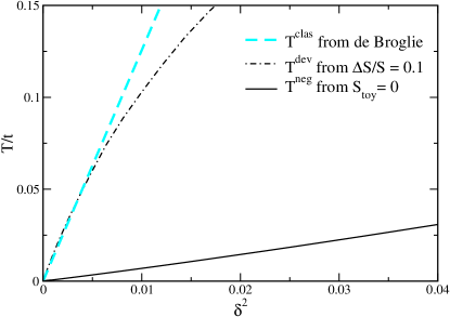
Figure 4: (color online) The toy model calculation differs from the exact fermionic calculation at low temperatures. The temperatures $T^{\rm dev}$ and $T^{\rm min}$ characterizing the limit of the approximate thermodynamics are plotted versus $\delta^{2}=(1-n)^{2}$. For comparison, $T^{\rm clas}$ resulting from the thermal de Broglie wave length $\lambda$ is included. For further details see main text.

The results for this toy model calculation are depicted in Fig. 3a in comparison to the entropy from the exact formula for non-interacting fermions. Discrepancies are found to be increasing with doping. They appear especially at low temperatures.

Since the deviations are small the relative deviation $\Delta S/S=(S_{\text{toy}}-S_{\text{TG}})/S_{\text{TG}}$ is plotted in Fig. 3b. For $n=0.8$ the difference of the entropies has a maximum at $T/t\approx 0.08$, then it drops and becomes even negative at very low temperatures because $S_{\text{toy}}$ becomes negative for $T\to 0$. This is an unphysical artifact of the approximate thermodynamics for hardcore bosons. For $n\rightarrow 1$ the maximum of the relative deviation is lower and shifted to lower temperatures. But artificial negative entropy behavior is still found for very low $T$.

To investigate systematically, below which temperature the approximate thermodynamics becomes significantly wrong, we define the temperature $T^{\rm dev}$, at which the relative deviation $\Delta S/S$ exceeds $10\%$. It is displayed in Fig. 4 as a function of $\delta^{2}=(1-n)^{2}$. In addition, the temperature $T^{\text{neg}}$ is shown which is defined as the temperature where the entropy of the toy model becomes negative. The temperatures $T^{\text{dev}}$ and $T^{\text{neg}}$ characterize the limit of applicability of the approximate thermodynamics.

Both temperatures are compared in Fig. 4 to the temperature $T^{\text{clas}}$ which results from equating the thermal de Broglie wave length

$$\lambda_{T}=\hbar\sqrt{\frac{2\pi}{mk_{\text{B}}T}}$$ (25)

with the average distance $1/\delta$ between two hole excitations $h$. The inverse mass $1/m$ is given by $2t$ which is the value of the second derivative at the band minimum. The excellent agreement in the proportionality $T\propto\delta^{2}$ and the very good agreement of $T^{\text{clas}}$ and $T^{\text{dev}}$ clearly show that the approximate thermodynamics is a classical treatment, which is valid as long as the gas of excitations is dilute enough. This argument quantifies the limitations of the approximate thermodynamics. For very low temperatures the results become unphysical. On the other hand, it shows that the results obtained for intermediate and high temperatures agree very well with the exact behavior in the TG regime.

IV.4 Results

In Sect. III, we have already learned that the temperature of the bosons in the optical lattice depends strongly on the regime of the system (Mott insulator or TG regime). The crucial point is whether the energetically low-lying states realize the initially present entropy or not. In the following, we investigate the entropy at finite $t/U$ for the effective model obtained by the CUT calculation and evaluated at finite temperatures by the approximate statistics for hardcore bosons.

In the limit of small $t/U$, the CUT can be performed straightforwardly. The results for the Mott phase are obtained for commensurate filling $n=1$. For fillings $n\neq 1$ the reference state used for normal ordering before truncation should ideally be the disordered state at the lower filling $n$ Reischl et al. (2005); Knetter et al. (2003). This requires to redo the whole CUT for each $n$. But the effect of a different reference state is not very large if $t/U$ is small. So our approach is to perform the CUT with the reference state (19) at $n=1$ as described in detail in Ref. Reischl et al., 2005. Note that this approach is exact as long as the CUT is performed without any approximation. So it does not represent an additional approximation in itself. The deviation from $n=1$ is included only on the level of the approximate thermodynamics of hardcore bosons described in Sect. IV.2. By tuning the chemical potential in Eq. 30 the average number of holes can be changed. This way of accounting for doping works particularly well for $n\approx 1$.

The entropy per site for the Bose-Hubbard system is calculated from the Gibbs energy (22) as $s=S/N=-\left.\frac{\partial g}{\partial T}\right|_{\mu}$. First, the entropy in the TG regime is discussed. In Fig. 5, the results for the entropy per particle from the CUT are compared to the results for the TG regime. The figure shows results for $t/U=0.01$ and $t/U=0.02$ corresponding to large values of the parameter $\gamma=U/t$ where the TG gas is realized Paredes et al. (2004); Wessel et al. (2005). The thick dotted curve shows the entropy per particle for $t/U=0.01$ for filling $n=1$. The increase of entropy with temperature is much slower for $n=1$ than for fillings $n=0.9$ (black curves) and $n=0.8$ (gray/cyan curves). For filling $n=0.9$, a very good agreement is found for low temperatures. The results based on CUT and on the approximate thermodynamics reproduce nicely the entropy in the TG regime. Good agreement is found up to temperatures of $T/t\approx 10$. For these temperatures, the TG result has already saturated at its high temperature limit. On the other hand, the CUT results begin to feel the presence of particle states (double occupancies in terms of the original bosons) which are not included in the TG description. Thus the CUT results deviate from the TG ones. The entropy is plotted versus $T/t$ in Fig. 5. A temperature of $10t$ corresponds to $T/U=0.1$ for $t/U=0.01$ but to $T/U=0.2$ for $t/U=0.02$. This is why the results for $t/U=0.02$ show deviations already for $T/t\approx 5$. A similar behavior is seen for $n=0.8$.

The small deviations discernible at low temperatures ($T\approx t$) must be attributed to the difference between the effective model obtained from the CUT and the simple fermionic tight-binding model with nearest-neigbor hopping only in the TG regime.

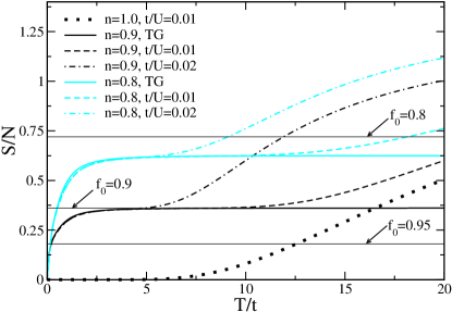
Figure 5: (color online) Entropy per particle in the TG regime. For small temperatures, the results from the CUT and the free Fermion calculation agree. At higher temperatures there are deviations caused by the presence of double occupancies in the bosonic Hubbard model.

Finally, Fig. 6 displays the entropy from the CUT calculation as function of temperature in units of $U$. The entropy per site for the undoped case is shown in Fig. 6 for three values of $t/U$ (black curves). The entropy does not change significantly for the values of $t/U$ that are shown because all of them are still deep in the Mott insulating phase.

The entropy per particle for condensate fractions $f_{0}=\{0.95;0.9;0.8\}$ is included as horizontal lines in Fig. 6. Assuming such condensate fractions and a hopping parameter $t/U=0.02$ the corresponding temperatures are $0.12;0.16;0.27$ in units of the interaction parameter $U$. These values are within the range of temperatures that were found by the analysis of spectral weights Reischl et al. (2005).

The influence of doping is shown in Fig. 6 by cyan (gray) curves for $n=0.9$. Clearly, several differences can be identified. At finite doping and small $t/U$, the constant entropy plateau seen for $t/U=0$ in Fig. 1 can still be recognized but there are changes for small temperatures of the order $t$. There is a finite dispersion at any finite $t$. Therefore, the entropy at zero temperature is zero because the macroscopic groundstate degeneracy is lifted. For increasing $t$ the plateau is washed out. At very low temperatures, there is a sharp uprise from zero entropy to a reduced entropy value comparable to the value realized at the plateau in the atomic limit. At higher temperatures, the entropy is dominated by the particle states (double occupancies) in analogy to what was found in the undoped case.

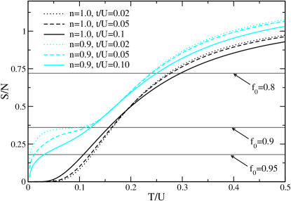
Figure 6: (color online) Entropy per particle as function of temperature for $t/U={0.02,0.05,0.1}$ at zero doping (black curves) and finite doping $n=0.9$ (cyan/gray curves). In addition, the value for the entropy per particle of the three dimensional harmonic oscillator with condensate fraction $f_{0}={0.8,0.9,0.95}$ is given.

V Conclusions

The main purpose of this work was to clarify the different orders of magnitude of temperature in recent experiments on the Mott insulating phase of ultracold bosons loaded adiabatically in one-dimensional optical lattices. On the one hand, temperatures of the order $U$ are found for the undoped Mott insulating phase Stöferle et al. (2004); Reischl et al. (2005). On the other hand, temperatures of the order $t$ are found in the TG regime.

By thermodynamic considerations, we found a physically relative simple and consistent picture. In the undoped Mott insulator, the temperature has to be of the order $U$. The groundstate is a single state and does not provide any entropy. The initially present entropy has to be realized by excited states. This requires a large temperature of the order of the gap. The situation is different for the doped Mott insulator. Already at the energy scale of the hopping an appreciable amount of entropy is possible due to the finite amount of holes or particles.

In comparison to experiment, an item still missing in our treatment is the inhomogeneity of the trap. So one might wonder whether our qualitative conclusions apply to the realistic systems. This question can be answered positively because it has been shown previously that the groundstate displays constant density plateaus at small values of $t/U$ Batrouni et al. (2002); Kollath et al. (2004). For zero or low temperature, the realistic situation can be seen as an ensemble of homogeneous systems of various fillings Batrouni et al. (2005). Thus it is expected that our qualitative conclusions concerning the orders of magnitude of temperature remain valid even if the inhomogeneity of a wide trap is taken into account.

The results were obtained on the one hand by considering limiting cases where a purely analytic treatment is possible and on the other hand by using a particle conserving CUT at zero temperature extended by an approximate thermodynamics for hardcore bosons. For the CUT the Bose-Hubbard Hamiltonian is reformulated in terms of a reference state with exactly one boson per site and excitations above this state. This approach yields reliable results in a wide parameter regime of the Mott insulating phase. Results at finite doping were obtained by tuning the chemical potential in the approximate hardcore thermodynamics. The reference state was not adapted to finite doping, which may represent a way to improve the CUT calculation. But we do not expect significant changes.

We tested the reliability of the approximate thermodynamics for hardcore bosons by comparison to the exact results in the TG regime which are based on the mapping of the system to non-interacting fermions. We find that the approximation works well up to relatively low temperatures $T>t/2$. We found that the approximate hardcore statistics corresponds to a classical description of the gas of hardcore particles. This results from the observation that the temperature below which the approximate statistics fails can be estimated to be the temperature at which the thermal de Broglie wave length $\lambda_{T}$ equals the interparticle distance.

Our considerations were restricted to one dimension because only in one dimension the hardcore bosons can be exactly mapped to fermions providing an easy-to-test benchmark. But apart from this generic one-dimensional feature used for the benchmark none of our arguments is restricted to one dimension. Thus we expect that the qualitative findings presented in this paper apply also to higher dimensions.

The obtained results provide a consistent picture of the role of temperature for bosons in one-dimensional optical lattices. We found that different physical situations can produce rather different temperatures. It is important in future experimental and theoretical works to take the influence of temperature into account in order to explore new quantum phenomena in the field of ultracold atoms.

VI Outlook

Our basic finding is that a restricted phase space at low energies leads inevitably to a relatively large temperature when the system is reached adiabatically from a Bose-Einstein condensate with a condensate fraction which deviates from unity. One obvious means to reach lower temperatures is to realize condensates with less entropy, i.e., with a higher condensate fraction $f_{0}$ at lower temperature.

Let us, however, suppose that this route cannot be used to reach the desired very low temperatures which are, for instance, necessary to perform reliable quantum computations. In such a case, we like to propose an alternative route. The system with very restricted phase space at low energies should be brought into weak thermal contact with another system in the optical trap which has a large phase space at low energies. Elementary thermodynamics tells us that the temperatures of both systems will finally become equal. This means that the system with large phase space cools the wanted system with small phase space down to low temperatures.

In the realm of bosons loaded in optical lattices this proposal means that one system should be realized which corresponds to a Mott insulator and which remains at relatively high temperatures in the adiabatic process because it does not have phase space below its gap. This Mott insulator can be cooled by a system which is in the TG regime, i.e., in the doped Mott insulating regime, with small hopping amplitude $t$. The TG system can accommodate for an appreciable amount of entropy even at low temperatures. Thus it is well-suited to cool the other system.

We cannot devise an experimental system which realizes the above idea. The use of two different laser systems in spatial vicinity for the same kind of atoms is certainly cumbersome. So it might be more promising to use two kinds of atoms in the same optical trap. The control parameters for the first kind of atoms should be such that it becomes Mott insulating upon loading into the optical lattice. The second kind should enter the TG regime upon loading. It is most challenging to see to how low temperatures a bosonic Mott insulating system can be pushed in such a way.

Appendix A Approximate Thermodynamics for Hardcore Bosons

This appendix provides the derivation of the approximate Gibbs energy of hardcore particles used in Sect. IV. The calculation adapts the reasoning in Ref. Troyer et al., 1994 for triplets in a spin ladder to the present hardcore excitations. The relevant excitations are independent particle and independent hole excitations. Multiple correlated $p$ and $h$ excitations and excitations of $d$-type are less relevant because of their higher energy. Therefore, we will neglect $d$-excitations and correlated excitations of more than one particle or hole in the following.

To use the non-interacting boson statistics for hardcore particles is a bad approximation because non-interacting bosons have no restriction on the occupation number. An incorrect number of states would contribute in the partition sum. The idea is to reweight all contributions to the partition sum such that they contribute the correct amount of entropy. Therefore we have to calculate the correct number of states with particle and hole excitations.

The number of possibilities to distribute $M$ truly bosonic excitations on $2L$ sites is

$$g_{\text{B}}(L,M)=\binom{2L+M-1}{M}.$$ (26)

But the correct number of possibilities of $M$ hardcore excitations of two kinds reads

$$g(L,M)=2^{M}\binom{L}{M}.$$ (27)

To obtain the correct entropy for each number of excitations the $M$-boson part in the partition sum is reweighted by the factor $g(L,M)/g_{\text{B}}(L,M)$. By this means, the partition function displays the correct high and low temperature behavior. The boson partition function for a system with $L$ sites and $M$ bosons is

$$Z^{\prime}(L,M)=\!\!\!\!\sum_{\stackrel{{\scriptstyle\{k_{j},k_{l}\}}}{{M=M_{p}+M_{h}}}}\!\!\!\!e^{-\beta\left(\sum_{j=1}^{M_{p}}\omega^{p}(k_{j})-\mu^{p}+\sum_{l=1}^{M_{h}}\omega^{h}(k_{l})-\mu^{h}\right)}.$$ (28)

The sum runs over all multi-indices $\{k_{j},k_{l}\}$ of $M=M_{p}+M_{h}$ momenta for particles at the momenta $\{k_{j}\}$ and holes at the momenta $\{k_{l}\}$. Here, $\omega^{p}(k_{j})$ is the energy of a particle with momentum $k_{j}$, $\omega^{h}(k_{l})$ the energy of a hole with momentum $k_{l}$. The chemical potential $\mu$ is accounted for by $\mu^{p}=\mu$ and $\mu^{h}=-\mu$. The negative sign in the definition of the chemical potential $\mu^{h}$ for holes results from the fact that adding a hole means removing an original boson. The boson partition function Eq. 28 contains $(2L)^{M}$ terms. Thus the reweighted partition function reads

$$\tilde{Z} = \sum_{M=0}^{L}\frac{g(L,M)}{(2L)^{M}}Z^{\prime}(L,M)$$ (29b)

$$= \sum_{M=0}^{L}L^{-M}\binom{L}{M}\!\!\!\!\sum_{\stackrel{{\scriptstyle\{k_{j},k_{l}\}}}{{M=M_{p}+M_{h}}}}$$

$$\qquad e^{-\beta\left(\sum_{j=1}^{M_{p}}\omega^{p}(k_{j})-\mu^{p}+\sum_{l=1}^{M_{h}}\omega^{h}(k_{l})-\mu^{h}\right)}\quad$$

$$= \left[1+L^{-1}\sum_{k;\sigma\in\{p,h\}}e^{-\beta(\omega^{\sigma}(k)-\mu^{\sigma})}\right]^{L}$$ (29c)

$$= \left[1+z^{p}+z^{h}\right]^{L}\ ,$$ (29d)

where we used the definition

$$z^{\sigma}:=\frac{1}{2\pi}\int_{0}^{2\pi}e^{-\beta(\omega^{\sigma}(k)-\mu^{\sigma})}dk$$ (30)

for the partition function of the single modes with $\sigma\in\{p,h\}$. The chemical potential $\mu$ is determined by specifying a certain filling. For instance, for the filling $n=1$ the chemical potential $\mu$ is determined such that as many particles as holes are excited.

We emphasize that Eq. 29 is only an approximation to the correct hardcore partition function because it contains contributions from states that are only allowed for non-interacting bosons, but are forbidden for hardcore bosons. The correct contribution of each subspace of fixed total number $M$ of excitations is ensured only in an overall manner by reweighting the total subspace.

Using the final expression (29d) one can compute the Gibbs energy per site $g$ to be

$$g=-(T/L)\ln\tilde{Z}=-T\ln(1+z^{p}+z^{h}).$$ (31)

Equations 30 and 31 are the formulae used in Sect. IV.2.

The toy model discussed in Sect. IV.3 includes only holes as possible excitations. Thus the Gibbs energy depends only on one partition function of a single mode $g_{\text{toy}}=-T\ln(1+z^{h})$. The dispersion of the toy model contains one single cosine-term $\omega^{h}(k)=-2t\cos(k)$ which makes the analytical calculation of $z^{h}$ possible

$$z^{h}=e^{\beta\mu^{h}}I_{0}(2\beta t)\ ,$$ (32)

where $I_{n}(z)$ is the modified Bessel function of the first kind. The entropy per particle reads

$$\frac{S}{N} = -\frac{1}{n}\left.\frac{\partial g}{\partial T}\right|_{\mu}$$ (34)

$$= -\beta e^{\beta\mu^{h}}\frac{2tI_{1}\left(2\beta t\right)+\mu^{h}I_{0}\left(2\beta t\right)}{n\left(1+e^{\beta\mu^{h}}I_{0}\left(2\beta t\right)\right)}$$

$$\qquad+\frac{1}{n}\log\left(1+e^{\beta\mu^{h}}I_{0}\left(2\beta t\right)\right)\ .\quad$$

References

- Jaksch et al. (1998) D. Jaksch, C. Bruder, J. I. Cirac, C. W. Gardiner, and P. Zoller, Phys. Rev. Lett. 81, 3108 (1998).
- Greiner et al. (2002) M. Greiner, O. Mandel, T. W. Hänsch, and I. Bloch, Nature 419, 51 (2002).
- Stöferle et al. (2004) T. Stöferle, H. Moritz, C. Schori, M. Köhl, and T. Esslinger, Phys. Rev. Lett. 92, 130403 (2004).
- Paredes et al. (2004) B. Paredes, A. Widera, V. Murg, O. Mandel, S. Fölling, I. Cirac, G. V. Shlyapnikov, T. W. Hänsch, and I. Bloch, Nature 429, 277 (2004).
- Kinoshita et al. (2004) T. Kinoshita, T. Wenger, and D. S. Weiss, Science 305, 1125 (2004).
- Köhl et al. (2005) M. Köhl, H. Moritz, T. Stöferle, C. Schori, and T. Esslinger, J. Low Temp. Phys. 138, 635 (2005).
- Reischl et al. (2005) A. Reischl, K. P. Schmidt, and G. S. Uhrig, cond-mat/0504724.
- Batrouni et al. (2005) G. G. Batrouni, F. F. Assaad, R. T. Scalettar, P. J. H. Denteneer, and M. Troyer, cond-mat/0503371.
- Krauth et al. (1992) W. Krauth, M. Caffarel, and J.-P. Bouchaud, Phys. Rev. B 45, 3137 (1992).
- Sheshadri et al. (1993) K. Sheshadri, H. R. Krishnamurthy, R. Pandit, and T. V. Ramakrishnan, Europhys. Lett. 22, 257 (1993).
- van Oosten et al. (2001) D. van Oosten, P. van der Straten, and H. T. C. Stoof, Phys. Rev. A 63, 053601 (2001).
- Fisher et al. (1989) M. P. A. Fisher, P. B. Weichman, G. Grinstein, and D. S. Fisher, Phys. Rev. B 40, 546 (1989).
- Elstner and Monien (1999) N. Elstner and H. Monien, Phys. Rev. B 59, 12184 (1999).
- Krauth (1991) W. Krauth, Phys. Rev. B 44, 9772 (1991).
- Dickerscheid et al. (2003) D. B. M. Dickerscheid, D. van Oosten, P. J. H. Denteneer, and H. T. C. Stoof, Phys. Rev. A 68, 043623 (2003).
- Pai et al. (1996) R. V. Pai, R. Pandit, H. R. Krishnamurthy, and S. Ramasesha, Phys. Rev. Lett. 76, 2937 (1996).
- Kashurnikov and Svistunov (1996) V. A. Kashurnikov and B. V. Svistunov, Phys. Rev. B 53, 11776 (1996).
- Kühner and Monien (1998) T. D. Kühner and H. Monien, Phys. Rev. B 58, R14741 (1998).
- Kühner et al. (2000) T. D. Kühner, S. R. White, and H. Monien, Phys. Rev. B 61, 12474 (2000).
- Blakie and Porto (2004) P. B. Blakie and J. V. Porto, Phys. Rev. A 69, 013603 (2004).
- Girardeau (1960) M. Girardeau, J. Math. Phys. 1, 516 (1960).
- Tonks (2002) L. Tonks, Phys. Rev. 50, 955 (2002).
- Jordan and Wigner (1928) P. Jordan and E. Wigner, Z. Phys. 47, 42 (1928).
- Lieb and Liniger (1963) E. H. Lieb and W. Liniger, Phys. Rev. 130, 1605 (1963).
- Troyer et al. (1994) M. Troyer, H. Tsunetsugu, and D. Würtz, Phys. Rev. B 50, 13515 (1994).
- Knetter et al. (2003) C. Knetter, K. P. Schmidt, and G. S. Uhrig, J. Phys. A: Math. Gen. 36, 7889 (2003).
- Reischl et al. (2004) A. Reischl, E. Müller-Hartmann, and G. S. Uhrig, Phys. Rev. B 70, 245124 (2004).
- Knetter and Uhrig (2000) C. Knetter and G. S. Uhrig, Eur. Phys. J. B 13, 209 (2000).
- Wessel et al. (2005) S. Wessel, F. Alet, S. Trebst, D. Leumann, M. Troyer, and G. Batrouni, J. Phys. Soc. Jpn. Suppl. 74, 10 (2005).
- Batrouni et al. (2002) G. G. Batrouni, V. Rousseau, R. T. Scalettar, M. Rigol, A. Muramatsu, P. J. H. Denteneer, and M. Troyer, Phys. Rev. Lett. 89, 117203 (2002).
- Kollath et al. (2004) C. Kollath, U. Schollwöck, J. von Delft, and W. Zwerger, Phys. Rev. A 69, 031601(R) (2004).