How long does it take to pull an ideal polymer into a small hole?

Abstract

We present scaling estimates for characteristic times $\tau_{\rm lin}$ and $\tau_{\rm br}$ of pulling ideal linear and randomly branched polymers of $N$ monomers into a small hole by a force $f$. We show that the absorbtion process develops as sequential straightening of folds of the initial polymer configuration. By estimating the typical size of the fold involved into the motion, we arrive at the following predictions: $\tau_{\rm lin}(N)\sim N^{3/2}/f$ and $\tau_{\rm br}(N)\sim N^{5/4}/f$, and we also confirm them by the molecular dynamics experiment.

PACS: 05.40.-a; 05.70.-a; 87.15.He

There are models in physics - most famously exemplified by an Ising model - whose importance is not due to their practical applicability to anything in particular, but because they provide the much needed training ground for our intuition and for the development of our theoretical methods. In polymer physics, one of the very few such models is that of ideal polymer absorbtion into a point-like potential well. For a homopolymer in equilibrium, this is a clean yet interesting example of a second order phase transition homopolymer ; Eisenregler . For a heteropolymer, even in equilibrium, the problem is still not completely understood – see, for example, gr_sh ; nech_na ; madr ; step ; mathematically it is similar to the localization (pinning) transition in the solid-on-solid models with quenched impurities forg ; vannim ; alex .

Surprisingly enough, the dynamics of a polymer chain pulled into a potential well is almost not discussed at all. On the first glance, one might think that this dynamics should be related to the dynamics of coil-globule collapse DeGennes1 ; DeGennes2 ; klushin ; obukhov ; gold , but the similarity between these two problems is limited. Indeed, globule formation after an abrupt solvent quench begins by a simultaneous chain condensation on many independent nucleation centers, while the absorbtion process can be viewed as pulling of a polymer with a constant force into a single hole. Hence, only a single attractive center causes the chain condensation. In this sense, dynamics of absorbtion into a potential well is more similar to a driven polymer translocation through a membrane channel Kasianowicz ; Meller3 ; Storm ; kar1 ; kar2 .

To describe in words the polymer pulled into a hole, let us imagine a long rope randomly dropped at the desk top. Pull now the rope by its end down from the desk edge. It is obvious, and can be established through an experiment accessible even to theorists, that the rope does not move all at once. What happens is only a part of the rope moves at the beginning, such that a fold closest to the end straightens out. As soon as the first fold is straightened, it then transmits the force to the next fold, which starts moving, and so on. The rope sequentially straightens its folds, such that at any moment only part of the rope about the size of a current fold is involved in the motion, while the rest of the rope remains immobile.

In the present letter we show how this mechanism applies to an ideal homopolymer dynamics and how it sheds light on the physics behind scaling estimates kar2 for the relaxation times for both linear, $\tau_{\rm lin}$, and randomly branched, $\tau_{\rm br}$, polymers.

We address the problem on the simplest level of an ideal Rouse homopolymer of $N$ monomers, each of size $a$, embedded into an immobile solvent with the viscosity $\eta$. One end of the chain is put in the potential well (the ”hole”), and the polymer is pulled down to the hole with constant force $f$, acting locally on just one single monomer, the one currently entering the hole. We will be interested in the relaxation time $\tau$ of the complete pulling down of the entire polymer into the hole, we want to know how $\tau$ depends on polymer length $N$ and the pulling force $f$. Neglecting inertia, the balance of forces reads $f=f_{\rm fr}(t)$, where friction force $f_{\rm fr}$ should be linear in velocity $\frac{dn}{dt}$, with $n(t)$ being the number of monomers ‘swallowed by the hole’ by the time $t$. More subtly, friction coefficient must be proportional to the number of monomers $m(t)$ currently involved in the forced motion: $f_{\rm fr}=\eta\,a^{2}\,m(t)\frac{dn(t)}{dt}$. Our main task will be to estimate the length $m(t)$ involved in the motion for either linear or branched polymers.

In order to clarify our approach, let us compute the characteristic time $\tau$ of pulling down of an initially stretched linear polymer. In this case, all monomers move except those already absorbed in the hole, so $m(t)=N-n(t)$, and so the force balance condition reads

$$f=\eta\,a^{2}\,\left[N-n(t)\right]\frac{dn(t)}{dt}\ .$$ (1)

Upon integration, this yields

$$\tau_{\rm straight}=\frac{\eta\,a^{2}}{2f}\,N^{2}\ .$$ (2)

In terms of dependence on $N$, this result is similar to the Rouse relaxation time of a linear polymer, $\tau_{R}\simeq\tau_{0}N^{2}$, where $\tau_{0}\simeq\eta a^{3}/k_{B}T$, and $T$ is temperature. Our estimate, (2), remains valid as long as $\tau_{\rm straight}<\tau_{R}$, because in this case the initially straight polymer has no time to coil up on itself while being pulled up by the force $f$. Given the expression for $\tau_{\rm straight}$, (2), the condition $\tau_{\rm straight}<\tau_{R}$ translates into $f>k_{B}T/a$, the latter making an obvious sense: pulling force should be strong enough to cause significant stretching of every bond, or, in other words, Pincus blobs must be as small as of the order of one monomer Pincus_blobs .

Now we turn to more realistic dynamics starting from a Gaussian coil configuration, and look at $\tau_{\rm lin}(N)$. To begin with, let us consider a simple scaling estimate kar2 . First of all, we note that the only time scale relevant for the problem is the above mentioned Rouse time $\tau_{R}$, which is the time needed for the coil to diffuse over the distance about its own size, $R\sim aN^{1/2}$. With $\tau_{R}$ being the solitary relevant time scale, the absorbtion time should be written in the scaling form

$$\tau_{\rm lin}=\tau_{R}\phi\left(\frac{fR}{k_{B}T}\right)\ ,$$ (3)

where the factor $\phi$ can depend on all other relevant parameters only in the dimensionless combination $fR/(k_{B}T)$. The second step follows from the fact that the speed of the process, $N/\tau_{\rm lin}$, must be linear in the applied force, which means that the function $\phi(x)$ should be inversely proportional to its argument, $\phi(x)\sim 1/x$. This then yields

$$\tau_{\rm lin}\sim\tau_{R}\frac{k_{B}T}{fR}\sim\frac{\eta a^{2}}{f}N^{3/2}\ .$$ (4)

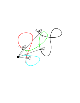
Scaling argument gives the answer, but does not give much insight. To gain proper insight, let us show how this same answer results from the process of sequential fold straightening. The definition of “folds” and of their lengths $s_{\rm fol}(N)$ is illustrated in Fig. 1. Since the chain is being pulled all the time into an immobile point in the center, the definition of a fold arises from considering only the radial component of the random walk, $\left|{\mathbf{r}}(s)\right|$, where ${\mathbf{r}}(s)$ stands for the (natural) parametric representation of a path. In $3D$, for example, $\left|{\mathbf{r}}(s)\right|$ represents Bessel random process bessel1 ; bessel2 . To obtain lengths of folds, $s_{\rm fol}^{(1)},\,s_{\rm fol}^{(2)},\ldots,\,s_{\rm fol}^{(k)}$, one has to coarse grain the trajectory up to the one monomer scale $a$, thus making a Wiener sausage, and then find the local minima of $\left|{\mathbf{r}}(s)\right|$ separated by the biggest maxima. It is obvious that there are about $\sqrt{N}$ of such minima, separated by the intervals about $\sqrt{N}$ each.

Figure 1: (Color online) Random coil viewed as a sequence of folds.

When we pull down the Gaussian chain by its end with a constant force $f$, only the current fold, of the length $s_{\rm fol}^{(i)}\sim\sqrt{N}$, is involved in the forced motion and experiences friction. The equation (1) is still valid, but $N$ should be replaced by $s_{\rm fol}^{(i)}$ and $n$ should be integrated in the limits $\left[0,s_{\rm fol}^{(i)}\right]$, yielding relaxation time for one fold

$$\tau_{\rm fol}=\frac{\eta\,a^{2}}{2f}\,\left(s_{\rm fol}^{(i)}\right)^{2}\sim\frac{\eta\,a^{2}}{f}N\ .$$ (5)

All $\sim\sqrt{N}$ folds relax sequentially, meaning that $\tau_{\rm lin}\sim\sqrt{N}\tau_{\rm fol}$, and thus returning the scaling answer (4).

Notice that the absorbtion time of a linear chain, $\tau_{\rm lin}$, Eq. (4), is much shorter than the typical Rouse time under the very weak condition $f>k_{B}T/(a\sqrt{N})$, which means Pincus blob dictated by the force $f$ should only be smaller than the entire coil. Under this condition, during the absorbtion process the configuration of the chain parts not involved into the straightening of a current fold, can be considered as quenched.

Figure 2: (Color online) Randomly branched chain and the corresponding hierarchy of scales.

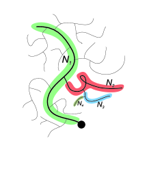
To understand the chain pulling dynamics even better, it is useful to consider another fundamental fractal model, that of randomly branched polymer, schematically shown in Fig.2. To find scaling approach for the randomly branched polymer, we have to estimate the analog of Rouse time as the time for a polymer to diffuse to its own size. Since all monomers experience friction independently of each other (there are neither solvent dynamics, nor hydrodynamic interactions), it follows that the diffusion coefficient of a Rouse coil, linear or branched, is given by $D\sim k_{B}T/(\eta aN)$. However, the radius of a branched polymer, unlike a linear one, is only $R\sim aN^{1/4}$. Therefore, the Rouse relaxation time for the branched polymer reads $\tau_{R}\sim\tau_{0}N^{3/2}$. The rest of the argument repeats exactly what we have done for the linear chain, yielding the result

$$\tau_{\rm br}\sim\tau_{R}\frac{k_{B}T}{fR}\sim\frac{\eta\,a^{2}}{f}N^{5/4}$$ (6)

Let us show now how one can re-derive (6) generalizing the concept of Bessel process to randomly branched chains. It is convenient to introduce a hierarchy of scales in the $N$–link ideal randomly branched chain. Let us denote by $N_{1}$ a number of monomers in a typical ”primitive” (or ”bare”) path of a largest scale. The size $R$ of an ideal randomly branched polymer is $R\sim aN^{1/4}$. The bare path of the maximal scale is a Gaussian random walk with $R\sim aN_{1}^{1/2}$. Hence, $N_{1}\sim N^{1/2}$. The average number of monomers in all side branches $N_{2},\,N_{3},\,N_{4}$, etc. attached to one bond of the bare path of the maximal scale (as shown in Fig.2a), is of order of $N/N_{1}\sim N^{1/2}$. All these side branches form a randomly branched configuration of size $R_{2}\sim a(N/N_{1})^{1/4}\sim aN^{1/8}$. Now, the number of monomers in the bare path of the second scale, $N_{2}$, can be obtained repeating the above scaling arguments: $R_{2}\sim aN_{2}^{1/2}$, giving $N_{2}\sim N^{1/4}$, and so on: $N_{3}\sim N^{1/8},\ldots,N_{k}\sim N^{2^{-k}}$,…– see Fig.2.

On all scales the bare paths $N_{1},N_{2},\ldots N_{k}$, etc. form the Gaussian sub-coils, each of which can be divided in folds $s_{\rm fol}^{(1)},\,s_{\rm fol}^{(2)},\ldots s_{\rm fol}^{(k)},\ldots$ in the same manner as it is done above for a linear chain. For $s_{\rm fol}^{(k)}$ we have the estimate

$$s_{\rm fol}^{(k)}\sim aN_{k}^{1/2}\sim aN^{2^{-(k+1)}}\qquad(k=1,2,\ldots)\ .$$ (7)

If the randomly branched polymer is pulled by its end with a constant force, $f$, then all Gaussian sub-coils on all scales straighten their folds simultaneously. The total typical number of monomers $s_{\rm all}$ in all folds simultaneously involved into the motion on all scales can be estimated as

$$s_{\rm all}\sim s_{\rm fol}^{(1)}s_{\rm fol}^{(2)}s_{\rm fol}^{(3)}...=aN^{1/4+1/8+1/16+\ldots}=aN^{1/2}\ .$$ (8)

We have seen on the example of the linear chain, that the characteristic time to straighten the fold of a typical length $s$ is of order of $\tau\sim s^{2}$ – see (5). So, as it follows from (8), the characteristic time of straightening out all folds of length $s_{\rm all}$ is of the order of

$$\tau_{\rm fol}^{\rm br}\sim\frac{\eta\,a^{2}}{2f}s_{\rm all}^{2}\sim\frac{\eta\,a^{2}}{f}N$$ (9)

In a randomly branched polymer there are $N_{1}a/s_{\rm fol}^{(1)}$ independent parts, which relax sequentially. Hence, the total relaxation time can be estimated as $\tau_{\rm br}\sim\left(\left.N_{1}a\right/s_{\rm fol}^{(1)}\right)\tau_{\rm fol}^{\rm br}$, which returns the result (6).

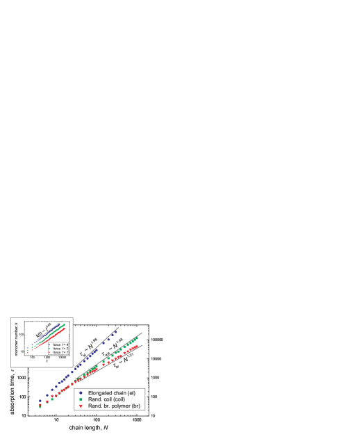
We have tested our results by a molecular dynamics experiment. We used standard Rouse model with harmonic bonds between neighboring monomers along the chain and with the averaged bond length, $a=1$. The attracting force $f$ acts at any moment on one monomer only and always points to the origin. Once a given monomer $k$ gets inside the absorbing hole ($|{\bf r}_{k}|<R_{a}=1$, where ${\bf r}_{k}$ is the position vector of the $k$th monomer) this monomer is considered absorbed, it does not move any more and does not exert any force on monomer $k+1$, its neighbor along the chain – but instead neighbor becomes the subject of the steady pulling force $f$. The same mechanism was simulated for the randomly branched polymer, except different branches can be pulled in parallel. The solution of dynamical equations is realized in the frameworks of the numerical velocity Verlet scheme verlet . The initial state of the linear chain was prepared by placing the first monomer at $|{\bf r}_{1}|=R_{a}$. The initial configuration of the randomly branched polymer was prepared as described in the work KCh , and then polymer was shifted as a whole to place one randomly chosen monomer on the absorbing surface $|{\bf r}|=R_{a}=1$. By performing 100 runs, we have computed averaged pulling times of linear chains from initially elongated and initially Gaussian conformations, as well as for a randomly branched polymer. The results are shown in the Fig. 3 and demonstrate very satisfactory agreement with the theoretical predictions (4) and (6).

In order to check more directly our proposed mechanism of absorption, we have looked at how Gaussian polymer chain gets involved into the biased motion driven by the pulling force $f$. The result is shown in the inset of figure 3. In this inset, $k(t)$, marks the crossover between current fold and the rest of the chain. The current fold is operationally defined to include all monomers, with numbers $j<k(t)$, whose motion is currently strongly affected by the pulling force $f$. Other monomers with the numbers $j>k(t)$ are not yet affected. The simulation indicates that thus defined $k(t)$ follows quite accurately the power law $k(t)\sim t^{2/3}$ with the exponent independent of the applied force. Inverting $k(t)$, we get $t\sim k^{3/2}$, which suggests that the time of complete absorbtion of a $k$-length subchain, which is given by our theoretical prediction (4), and the time of involving $k$-length subchain in the force-biased motion scale in the same way.

Figure 3: (Color online). Log-log plot of relaxation time against $N$. The units: $a=1$, $k_{B}T=1$, and $\eta=10$. Bullets ($\bullet$) – initially straightened linear chain, squares ($\blacksquare$) – initially coiled linear polymer, triangles ($\blacktriangle$) – randomly branched polymers. The slopes are consistent with theoretical predictions. Inset: time dependence of the $k(t)$ in the log-log scale. Here $k(t)$ is the monomer number such that at the given time moment $t$ monomers before $k$ are already strongly involved in the biased motion towards the absorbing hole, while monomers after $k$ are still diffusing not influenced by the force.

To conclude, we have considered scaling estimates of the relaxation time associated with pulling linear or randomly branched polymer chain into a hole by a constant force $f$. We found that these estimates, $\tau_{\rm lin}\sim(\eta\,a^{2}/f)N^{3/2}$ and $\tau_{\rm br}\sim(\eta\,a^{2}/f)N^{5/4}$, are consistent with the molecular dynamics simulation and they can be understood in terms of the scenario of sequential straightening of the polymer parts which we called folds and which were defined in terms of the radial component of the random walk representing the polymer chain.

We have to emphasize that all consideration in this paper was restricted to polymer models without excluded volume in 3D. There is no doubt that self-avoidance, as well as hydrodynamic interactions will significantly affect the specific scaling relations obtained here. The account of excluded volume effects is, to some extent, simpler than that of hydrodynamic interactions. On the basis of scaling approach we can predict the pulling time, $\tau(N)\sim N^{1+\nu}/f$, for the polymer characterized by the exponent $\nu$ in the relation $R\sim N^{\nu}$. Our consideration is also restricted in the sense that we did not consider the role of the polymer part already ‘swallowed’ by the potential well. Although this might affect the result under some conditions, our aim was to elucidate the mechanism of sequential straightening of folds, for that purpose the absorbed tail is irrelevant. Similarly, in reality polymer is usually pulled into a hole in a wall, such as membrane, and we have neglected the (presumably logarithmic) factors associated with the excluded half-space.

However, as we said in the beginning, the purpose of the model is to facilitate methods and intuition. In this sense, we think that the consideration of ideal polymer in this letter was fruitful, because the mechanism of sequential straightening of folds obviously applies to a number of real physical situations, such as, e.g., DNA translocation through the membrane pore driven by the difference in chemical potentials.

AYG gratefully acknowledges warm hospitality he felt throughout his stay at the LPTMS where this work was done. This work is partially supported by the grant ACI-NIM-2004-243 ”Nouvelles Interfaces des Mathématiques” (France).

References

- (1) K. Binder, in Phase Transitions and Critical Phenomena, vol. 10, ed. C. Domb and J. Lebowitz (New York: Academic, 1983)
- (2) Polymers Near Surfaces, (Singapore: WSPC, 1993)
- (3) A.Yu. Grosberg, E.I. Shakhnovich, Sov. Phys. JETP 64, 1284 (1986)
- (4) A.Naidenov, S. Nechaev, J. Phys. A: Math. Gen. 34, 5625 (2001)
- (5) N. Madras, S.G. Whittington, J. Phys. A: Math. Gen. 35, L427 (2002)
- (6) S. Stepanow, A.L. Chudnovskiy, J. Phys. A: Math. Gen. 35, 4229 (2002)
- (7) G. Forgas et al, in Phase Transitions and Critical Phenomena eds. C. Domb and J Lebowitz (New York: Academic, 1991)
- (8) J. Vannimenus, B. Derrida, J. Stat. Phys. 105, (2001) 1
- (9) K.S. Alexander, V. Sidoravicius, eprint arXiv:math/0501028
- (10) P.G. de Gennes J. de Physique Lett. 46, L639 (1985)
- (11) A.Buguin, F.Brochard-Wyart, P.G.de Gennes, CR Acad. Sci. Paris, 322 IIb, 741 (1996)
- (12) L. L. Klushin, J. Chem. Phys. 108, 7917 (1998).
- (13) C. F. Abrams, N. Lee, S. Obukhov, Europhys. Lett., 59, 391 (2002)
- (14) A. Halperin, P. M. Goldbart, Phys. Rev. E 61, 565 (2000)
- (15) J.J. Kasianowicz, E. Brandin, D. Branton, and D.W. Deamer, Proc. Natl. Acad. Sci. U.S.A. 93, 13770 (1996).
- (16) A. Meller, L. Nivon, and D. Branton, Phys. Rev. Lett. 86 3435 (2001).
- (17) A.J. Storm, C. Storm, J. Chen, H. Zandbergen, J.F. Joanny, and C. Dekker, Nano Lett. 5, 1193 (2005).
- (18) J. Chuang, Y. Kantor, M. Kardar, Phys. Rev. E 65, 011802 (2002)
- (19) Y. Kantor, M. Kardar, Phys. Rev. E 69, 021806 (2004)
- (20) P. Pincus, Macromolecules, 9, 386 (1976)
- (21) M. Donsker, S.R.S. Varadhan, Comm. Pure Appl. Math, 28, 525 (1975)
- (22) J.D. Pitman, M. Yor, ”Bessel process and infinetely divisible laws, in Stochastic integrals, ed. D. Williams, Lecture Notes in Mathematics, vol. 851 (Berlin: Springer, 1981)
- (23) A.N. Borodin, P. Salminen, Handbook of Brownian motion – Facts and Formulae, 2nd ed. (Basel: Birkhäuser, 2002)
- (24) W.C. Swope, H.C. Andersen, P.H.Berens, K.R. Wilson, J. Chem. Phys., 76, 673 (1982)
- (25) J.P. Kemp, Z.Yu. Chen, Phys. Rev. E 60, 2994 (1999)