Field dependence of magnetic ordering in Kagomé-staircase compound ${\bf Ni_{3}V_{2}O_{8}}$

Abstract

We present powder and single-crystal neutron diffraction and bulk measurements of the Kagomé-staircase compound ${\rm Ni_{3}V_{2}O_{8}}$ (NVO) in fields up to $8.5$T applied along the c-direction. (The Kagomé plane is the a-c plane.) This system contains two types of Ni ions, which we call “spine” and “cross-tie”. Our neutron measurements can be described with the paramagnetic space group ${\rm Cmca}$ for $T<15$K and each observed magnetically ordered phase is characterized by the appropriate irreducible representation(s). Our zero-field measurements show that at $T_{\rm PH}=9.1$K NVO undergoes a transition to an incommensurate order which is dominated by a longitudinally-modulated structure with the spine spins mainly parallel to the a-axis. Upon further cooling, a transition is induced at $T_{\rm HL}=6.3$K to an elliptically polarized incommensurate structure with both spine and cross-tie moments in the a-b plane. At $T_{\rm LC}=4$K the system undergoes a first-order phase transition, below which the magnetic structure is a commensurate antiferromagnet with the staggered magnetization primarily along the a-axis and a weak ferromagnetic moment along the c-axis. A specific heat peak at $T_{\rm CC^{\prime}}=2.3$K indicates an additional transition, which we were however not able to relate to a change of the magnetic structure. Neutron, specific heat, and magnetization measurements produce a comprehensive temperature-field phase diagram. The symmetries of the two incommensurate magnetic phases are consistent with the observation that only one phase has a spontaneous ferroelectric polarization. All the observed magnetic structures are explained theoretically using a simplified model Hamiltonian, involving competing nearest- and next-nearest-neighbor exchange interactions, spin anisotropy, Dzyaloshinskii-Moriya and pseudo-dipolar interactions.

I Introduction

Quantum spin systems with competing interactions can have highly-degenerate ground-state manifolds with unusual spin correlations. Small, otherwise insignificant perturbations can then become decisively important by removing the degeneracy of the low-energy spin fluctuations, leading to unexpected ground states at low temperatures. The proximity to quantum phase transitions, which separate the various ground states, can lead to new types of instabilities which involve charge and lattice degrees of freedom. Examples include exotic superconductivity, heavy-fermion conductors and ferroelectricity.

Frustrated low-spin magnets are ideal model systems for the study of competing quantum phases because they naturally contain competing interactions in a clearly-defined geometry. An important model system is the Kagomé lattice which consists of corner-sharing triangles of spins with equal antiferromagnetic (AF) coupling between nearest neighbors. Theoretically it is expected that the $S=\frac{1}{2}$ Kagomé lattice does not have long-range order at zero temperature, but adopts a quantum spin liquid ground state.Sachdev ; Sindzingre The most well known Kagomé-related magnet is the $S=\frac{3}{2}$ compound ${\rm SrCr_{9}Ga_{3}O_{19}}$. However, the structure is actually better described as a Kagomé bilayer with an intervening triangular latticeNEW and it has a ground spin-glass like ground state.BroholmAeppli ; RamirezEspinosa Work on jarosite systems showed various types of commensurate long-range order stabilized by inter-layer and Dzyaloshinskii-Moriya (DM) interactions.LeeBroholm ; YSLee These results indicate that Kagomé related magnets are highly sensitive to relatively weak interactions, and hence are a likely venue for new and exotic ordered states.

${\rm Ni_{3}V_{2}O_{8}}$ (NVO) is a system of weakly-coupled spin-1 staircase Kagomé planes containing two types of inequivalent bonds and magnetic sites. It is thus a variant of the highly-frustrated pure Kagomé lattice. However, these deviations from ideal Kagomé geometry introduce several new interactions which determine how the quantum degeneracy and frustration are resolved. In addition, it has been foundFERRO that the magnetic ordering generates ferroelectricity and these smaller interactions play a crucial role in this phenomenon and can explain the microscopic origins of multiferroics.TOBE

Magnetic susceptibility and specific heat measurements reveal that NVO undergoes a series of magnetic phase transitions with temperature and magnetic fieldRogado ; LawesKenzelmann and in Fig. 1 we reproduce the phase diagram as found in Ref. LawesKenzelmann, , which we refer to as I. There, our neutron diffraction study at zero field showed that NVO adopts two different incommensurate phases above $4$K, a mainly longitudinal incommensurate phase which occurs at higher temperature (which we therefore call the high-temperature incommensurate, HTI, phase) and a spiral incommensurate phase which occurs at lower temperature and which we call the low-temperature incommensurate, or LTI, phase. We also found evidence of a commensurate canted AF phases below $4$K. One purpose of this paper is to present a comprehensive review of neutron diffraction data which enables us to characterize the HTI, LTI and C phases, but we will not discuss in detail the C’ phase. A second purpose is to show that the phase diagram can be understood to be the result of competing nearest-neighbor (nn) and next-nearest-neighbor (nnn) exchange interactions, easy-axis anisotropy, and anisotropic interactions, both pseudo-dipolar (PD) as well as DM interactions. It is particularly important to characterize the magnetic structure of NVO in order to gain an understanding of the magnetoelectric couplingFERRO which causes the LTI phase to be ferroelectric.

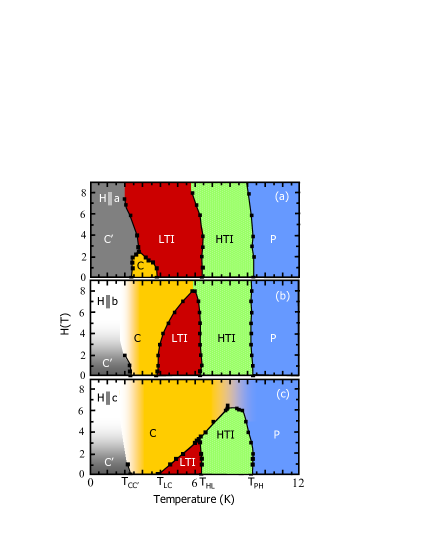
Figure 1: Phase diagram in $H$-$T$ when ${\bf H}$ is applied along each of the three crystallographic axes. This phase diagram is based on specific heat data taken as a function of $T$ at constant $H$ (Ref LawesKenzelmann, ). The phases are labeled P for the paramagnetic (magnetically disordered) phase, HTI for the high-temperature incommensurate phase, LTI for the low-temperature incommensurate phase, C for the high-temperature canted AF phase, and C’ for the low-temperature canted AF phase. The spin structures of these phases are described below. The transition temperatures (in order of decreasing temperature) are denoted $T_{\rm PH}$, $T_{\rm HL}$, $T_{\rm LC}$, and $T_{\rm CC^{\prime}}$. For a field along ${\bf c}$, the C and P phases have the same symmetry, and therefore there is no sharp transition between them.

The experimental details, data analysis, and physical interpretation which were only briefly presented in I, are fully explained in this paper. We performed a zero-field powder and single-crystal neutron diffraction study to determine the magnetic structures, and we used group theory to identify the structures that are allowed by symmetry for the two observed ordering wave-vectors. Further we present the field dependence of the magnetic structures by monitoring AF and ferromagnetic (FM) Bragg peaks. Magnetic fields up to $8.5$T were applied along the crystallographic $\bf c$-direction. We find that application of a magnetic field along the $\bf c$-axis favors the AF C phase at the expense of the incommensurate phases. Thus the phase diagram obtained by our neutron diffraction experiments is consistent with that obtained from macroscopic measurements, some of which are presented here and provide additional information on the microscopic interactions between magnetic ions.

Almost all our results can be understood on the basis of theoretical models that are analyzed in detail in a separate paper,THEORY which we refer to as II. To avoid undue repetition we will here indicate in qualitative terms how these models explain the data and we refer the reader to II for quantitative details.

Briefly this paper is organized as follows. In Sec. II we summarize the experimental techniques used in this work. In Sec. III we give our determination of the crystal crystal which confirms earlier work by Sauerbrei et al.Sauerbrei Section IV contains the magnetic structure determinations. Here we give a brief summary of representation theory, since this forms the basis for almost all the structure determinations. We also present magnetization and susceptibility data for magnetic fields applied along the three crystallographic directions. In Sec. VI we give a theoretical interpretation of the experimental results. We obtain rough estimates of many of the microscopic interaction parameters using the more detailed calculations presented in II. Finally, our results are summarized in Sec. VI.

II Experimental

Powder samples of NVO were made in a crucible using ${\rm NiO}$ and ${\rm V_{2}O_{5}}$ as starting materials.Rogado Single crystals were grown from a ${\rm BaO}$-${\rm V_{2}O_{5}}$ flux.LawesKenzelmann Neutron diffraction experiments were performed using a powder sample with a total mass of $10\;\mathrm{g}$ and a single crystal with a mass of $0.13\;\mathrm{g}$ oriented with the $(h,k,0)$ or $(h,k,k)$ crystallographic planes in the horizontal scattering plane of the spectrometers.

Powder neutron measurements were performed using the BT-1 high-resolution powder diffractometer at the NIST Center for Neutron Research, employing Cu (311) and Ge (311) monochromators to produce a monochromatic neutron beam of wavelength $1.5401$Å and $2.0775$Å, respectively. Collimators with horizontal divergences of $15^{\prime}$, $20^{\prime}$, and $7^{\prime}$ were used before and after the monochromator, and after the sample, respectively. The intensities were measured in steps of $0.05^{o}$ in the range of scattering angles, $2\Theta$, from $3^{o}$ to $168^{o}$. Data were collected at various temperatures from $1.5$K to $30$K to elucidate the temperature dependence of the crystal structure. The program GSAS GSAS was used to refine the structural parameters and the commensurate magnetic structure. Additional diffraction data and magnetic order parameters were obtained on the BT7 triple axis spectrometer to explore the magnetic scattering in more detail. For these measurements, a pyrolytic graphite PG(002) double monochromator was employed at a wavelength of $2.47$Å, with $40^{\prime}$ collimation after the sample and no analyzer.

		$T=15$K	$T=1.5$K
a (Å)		5.92179(3)	5.92197(3)
b (Å)		11.37105(7)	11.37213(7)
c (Å)		8.22638(5)	8.22495(5)
${\rm Ni_{s}}$	y	0.1299(1)	0.1299(1)
	B(Å2)	0.26(1)	0.24(1)
${\rm Ni_{c}}$	B(Å2)	0.24(2)	0.28(2)
V	y	0.3762	0.3762
	z	0.1196	0.1196
	B(Å2)	0.24	0.24
${\rm O_{1}}$	y	0.2482(2)	0.2482(2)
	z	0.2308(2)	0.2309(2)
	B(Å2)	0.31(2)	0.30(2)
${\rm O_{2}}$	y	0.0012(2)	0.0008(2)
	z	0.2443(2)	0.2447(2)
	B(Å2)	0.32(2)	0.31(2)
${\rm O_{3}}$	x	0.2656(2)	0.2660(2)
	y	0.1190(1)	0.1191(1)
	z	0.00039(8)	0.00029(8)
	B(Å2)	0.34(2)	0.30(2)
$R_{\rm p}$ (%)		3.80	3.97
$R_{\rm wp}$(%)		4.69	4.78
$\chi^{2}$		1.245	1.294
		distances in $\AA$
${\rm Ni_{s}}$-${\rm O_{2}}$	2	2.010(2)	2.013(2)
${\rm Ni_{s}}$-${\rm O_{3}}$	4	2.075(2)	2.078(1)
${\rm Ni_{c}}$-${\rm O_{1}}$	2	2.006(2)	2.006(2)
${\rm Ni_{c}}$-${\rm O_{2}}$	2	2.083(1)	2.085(1)
${\rm Ni_{c}}$-${\rm O_{3}}$	2	2.0599(7)	2.0597(7)
${\rm Ni_{s}}$-${\rm Ni_{c}}$	4	2.9330(6)	2.9331(6)
${\rm Ni_{c}}$-${\rm Ni_{c}}$	2	2.96089(2)	2.96098(2)

Table 1: Structural parameters and selected interatomic distances for NVO, measured using the BT1 spectrometer with the Ge (311) monochromator and $\lambda$=$2.0775$Å. Space group: Cmca (No. 64 in Ref. HAHN, ). Atomic positions (expressed as fractions of $a$, $b$, and $c$): ${\rm Ni_{s}}$: 8e (notation as in Ref. HAHN, ) ($\frac{1}{4}$, y, $\frac{1}{4}$); ${\rm Ni_{c}}$: 4a (0 0 0 ); V: 8f (0 y z ); ${\rm O_{1}}$: 8f (0 y z ); ${\rm O_{2}}$: 8f (0 y z ); ${\rm O_{3}}$: 16g (x y z ). $B_{i}\equiv 8\pi^{2}\langle u_{i}^{2}\rangle$, where $u_{i}$ is the displacement of atom $i$ from its equilibrium position and $\langle...\rangle$ indicates a thermal average. Also $R_{\rm p}$=$\sum^{n}_{i}|I^{i}_{o}-I^{i}_{c}|/\sum_{i}I^{i}_{o}$ where $I^{i}_{o}$ and $I^{i}_{c}$ are the $n$ observed and calculated intensities, respectively. $R_{\rm wp}$=$\sqrt{\sum w_{i}(I^{i}_{o}-I^{i}_{c})^{2}/\sum w_{i}(I^{i}_{o})^{2}}$ where the weight is given by $w_{i}$=$1/\sigma^{2}_{i}$. The sum of least-squares is given by $\chi^{2}$=$\sum^{n}_{i}w_{i}(|F^{i}_{o}|-|F^{i}_{c}|)^{2}/(n-m)$, where $m$ is the number of fitted variables.

The single-crystal neutron scattering measurements were performed with the thermal-neutron triple-axis spectrometers BT7 and BT9, and with the cold-neutron triple-axis spectrometer SPINS. The BT7 experiment was performed with 60’ collimation after the sample, a PG(002) analyzer to reflect $13.408\;\mathrm{meV}$ neutrons and 180’ beam divergence after the analyzer. The BT9 diffraction measurements were performed with an incident energy of $30.5\;\mathrm{meV}$ and 40’-40’ collimation around the sample. The $H$-$T$ magnetic phase diagram was determined using SPINS with an incident energy of $5\;\mathrm{meV}$, a Be filter before the sample and 80’-80’ collimation around the sample. The SPINS diffraction patterns were collected with 80’-80’ collimation around the sample, a PG(004) monochromator combined with a graphite filter in the incident beam and a flat PG(002) analyzer set for $14.7\;\mathrm{meV}$. The beam divergence between analyzer and detector was 240’.

III Nuclear structure

III.1 Experimental determination of structure

The NVO structure refinement from BT1 neutron powder diffraction data was carried out successfully using the previously reported structural parametersSauerbrei as initial values. In agreement with previous studies, we found the structure to have Cmca symmetry (space group No. 64 in the International Tables for CrystallographyHAHN ). No structural transition was detected for 1.5K$<T<$300K. The structural parameters and selected interatomic distances at two temperatures are given in Table 1. The symmetry elements of the Cmca space group of NVO are given in Table 2. Because V has a low coherent neutron scattering cross-section, the atomic positions and temperature factors of the vanadium ions were fixed to the values obtained by Xray diffraction.Sauerbrei

${\rm E}{\bf r}=(x,y,z)$	$2_{c}{\bf r}=(\overline{x},\overline{y}+1/2,z+1/2)$
$2_{b}{\bf r}=(\overline{x},y+1/2,\overline{z}+1/2)$	$2_{a}{\bf r}=(x,\overline{y},\overline{z})$
${\cal I}{\bf r}=(\overline{x},\overline{y},\overline{z})$	$m_{ab}{\bf r}=(x,y+1/2,\overline{z}+1/2)$
$m_{ac}{\bf r}=(x,\overline{y}+1/2,z+1/2)$	$m_{bc}{\bf r}=(\overline{x},y,z)$

Table 2: General positions within the primitive unit cell for Cmca which describe the symmetry operations of this space group. $2_{\alpha}$ is a two-fold rotation (or screw) axis and $m_{\alpha\beta}$ is a mirror (or glide) $\alpha-\beta$ plane.

To investigate the effect of magnetic ordering on the chemical structure, a series of powder patterns were taken below $10$K. No significant change for the a-axis, unit cell volume, and Ni-O bond distances were observed, as shown in Fig. 2 and Table 1. However, reducing the temperature below $10$K leads to an increasing $b$ lattice parameter, while the $c$ lattice parameter decreases without a change in space group symmetry.

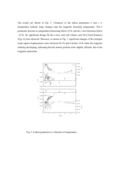
Figure 2: Lattice parameters $a$, $b$, and $c$ as a function of temperature, determined from neutron powder diffraction using BT1 with a Cu (311) monochromator and a wavelength 1.5401Å. Also shown is the temperature dependence of the unit cell volume.

The strongest temperature dependence is associated with the isotropic mean-square displacements for Ni and O, which change significantly with the onset of commensurate order at $4$K (Fig. 3). This may indicate a weak coupling of the magnetic and the chemical lattice. However, we did not observe a crystal distortion with the given neutron diffraction resolution. Higher-resolution xray or neutron diffraction would be needed to look for possible space group symmetry breaking associated with the onset of commensurate order.

III.2 Structural properties

Here we note some general features of the structure. The structure of NVO consists of ${\rm Kagom\acute{e}}$ layers of edge-sharing ${\rm NiO_{6}}$ octahedra. The layers are separated by nonmagnetic ${\rm V^{5+}O_{4}}$ tetrahedra. There are two inequivalent crystallographic sites for Ni, denoted as ${\rm Ni_{s}}$ and ${\rm Ni_{c}}$. (We will refer to these as “spine” and “cross-tie” sites, respectively.) At $15$K, the average ${\rm Ni^{2+}-Ni^{2+}}$ distance within the layers is $d_{1}=2.94$Å, while the inter-layer distance is $d_{2}=5.69$Å. Based on the relatively large inter-layer to intra-layer ratio, $d_{2}/d_{1}=1.9$, a strong two-dimensional magnetic character may be expected in this compound, with the magnetism dominated by intra-layer ${\rm Ni^{2+}-Ni^{2+}}$ exchange interactions. Unlike previously studied ${\rm Kagom\acute{e}}$ lattice-based materials, which have planar magnetic layers, the Ni-O layers in NVO are buckled, resulting in the “${\rm Kagom\acute{e}}$-staircase” structure. The symmetry of the superexchange interaction mediated by O ions shows that there are two inequivalent superexchange paths between neighboring ${\rm Ni^{2+}}$ ions within ${\rm Kagom\acute{e}}$ planes. In particular, there is a superexchange path between ${\rm Ni_{s}}$ positions along the crystallographic a-direction which is different from nn interactions between Ni ions on neighboring ${\rm Ni_{s}}$ and ${\rm Ni_{c}}$ positions.

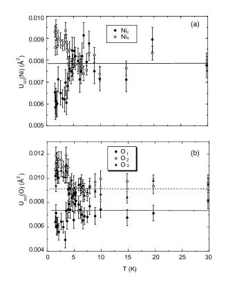
Figure 3: Isotropic mean-square displacements of Ni and O as a function of temperature, obtained from the same powder spectra mentioned in Fig. 2.

The point group is Abelian and its three generators are spatial inversion (${\cal I}$), and the two-fold rotations $R_{a}$ and $R_{b}$ about the $\bf a$ and $\bf b$ axes respectively. The space group operations are ${\cal I}$ and $R_{a}$ referred to the origin at a cross-tie site, such as site c1 in Fig. 4, and $R_{b}$ about an axis passing through a spine site such as site s1 in Fig. 4. The operations give rise to mirror planes perpendicular to the ${\bf a}$-axis passing through a cross-tie site and a two-fold screw axis about a $z$-axis passing through a spine site such as site s1 with a translation of $c/2$ along ${\bf c}$. There is a glide plane perpendicular to the $\bf c$-axis passing through a chain of spine sites with a translation $a/2$ along ${\bf a}$. The result of these symmetry operations is that all the Ni spine sites are related by symmetry and all the Ni cross-tie sites are similarly related by symmetry. Our convention for the coordinate axes is as follows: the spines lie along the (100), or a-axis (denoted sometimes the $x$-axis), the basal plane includes this axis and the (001), or c-axis (or sometimes the $z$ axis), and the axis perpendicular to this plane is denoted (010) or the b-axis (or sometimes the $y$-axis). The two types of Ni sites are shown in Fig. 4 and their coordinates are given in Table 3.

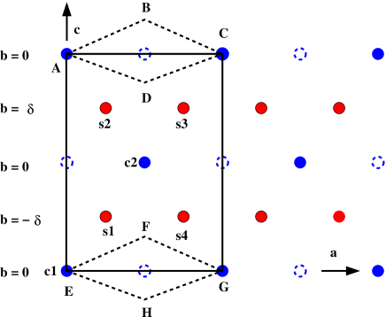
Figure 4: Ni sites in the primitive unit cell, whose vertices are A, B, …H and is defined by the vectors ${\bf v}_{1}=(a/2)\hat{a}+(b/2)\hat{b}$, ${\bf v}_{2}=(a/2)\hat{a}-(b/2)\hat{b}$, and ${\bf v}_{3}=c\hat{c}$. The “cross-tie” sites (on-line=blue) c1 and c2 lie in a plane with $b=0$. The “spine” sites (on-line=red) are labelled s1, s2, s3, and s4 and they may be visualized as forming chains parallel to the ${\bf a}$-axis. These chains are in the buckled plane with $b=\pm\delta$, where $\delta=0.13b$ as is indicated. Cross-tie sites in adjacent planes (displaced by $(\pm b/2)\hat{b}$) are indicated by open circles. Spine sites in adjacent planes are located directly above (or below) the sites in the plane shown.

	${\bf r}_{s}^{1}$	=	$(0.25,-0.13,0.25)$
	${\bf r}_{s}^{2}$	=	$(0.25,0.13,0.75)$
	${\bf r}_{s}^{3}$	=	$(0.75,0.13,0.75)$
	${\bf r}_{s}^{4}$	=	$(0.75,-0.13,0.25)$
	${\bf r}_{c}^{1}$	=	$(0,0,0)$
	${\bf r}_{c}^{2}$	=	$(0.5,0,0.5)$

Table 3: Positions of ${\rm Ni^{2+}}$ carrying $S$=$1$ within the primitive unit cell illustrated in Fig. 4. Each component is expressed as a fraction of the respective lattice constant, so ${\bf r}_{s}^{1}=0.25{\bf a}-0.13{\bf b}0.25{\bf c}$. Lattice positions ${\bf r}_{s}^{n}$ are spine sites and ${\bf r}_{c}^{n}$ are the cross-tie sites. NVO orders in space group ${\rm Cmca}$, so there are six more atoms in the orthorhombic unit cell which are obtained by a translation of lattice ${\bf r}_{1}$ through ${\bf r}_{6}$ by $(0.5,0.5,0)$.

The spine and cross-tie sites have different local symmetry and will be seen to have very different magnetic properties. In the presence of AF ordering of the spine sites, the cross-tie sites are frustrated if one assumes isotropic AF Heisenberg interactions; the sum of the moments of the four spine neighbors of each cross-tie spin vanishes. In this regard, this system is reminiscent of ${\rm Sr_{2}Cu_{3}O_{4}Cl_{2}}$ ChouAharony and of various “ladder” systems which have recently been studied.KiryukhinBirgeneau

The above structure has several implications for the magnetic interactions. As explained in Ref. Rogado, , the leading nn Ni-Ni magnetic coupling arises via superexchange interactions, mediated by two Ni-O-Ni bonds. For a pair of nn spine spins, the angles of these two bonds are 90.4^o and 95.0^o. For a spine-cross-tie pair, these angles are 90.3^o and 91.5^o. For the similar case of Cu-O-Cu bonds, it has been shown that when these angles are close to 90^o then the resulting exchange energy is small,Tornow and may even change its sign from FM to AF (as the angle decreases from 90^o). Since both Ni and Cu involve $d$-holes in the high $e_{g}$ states (within the oxygen octahedron surrounding Ni or Cu), we expect similar results to apply for the Ni case. Accordingly, we do not necessarily expect that nn interactions dominate second neighbor interactions. Similar calculations for the related nnn coupling, via Cu-O-O-Cu, gave AF interactions.Tornow Similar Ni-O-O-Ni interactions could compete with the nn interactions, and give rise to incommensurate structures, as explained below.

As a result of the crystal symmetries, there is a limited number of independent nn interaction matrices. If we write the interaction between spine spins ${\bf S}(i)$ and ${\bf S}(j)$ as

$${\cal H}_{ij} = \sum_{\alpha\beta}M_{\alpha\beta}(i,j)S_{\alpha}(i)S_{\beta}(j)\,,$$ (1)

where $\alpha=a,b,c$ is a component label, then once we have specified $M_{\alpha\beta}(s1,s4)$ (in the notation of Fig. 4), we can express the interaction matrices for all other nn pairs of spine sites in terms of $M_{\alpha\beta}(s1,s4)$. Similarly, we only need to specify a single interaction matrix, e. g. $M_{\alpha\beta}(s1,c2)$, for nn pairs of spine and cross-tie sites or for interactions between nnn in the same spine. Symmetry also places some restrictions on the form of $M_{\alpha\beta}(s1,s4)$. These results are obtained in II.

IV Magnetic structure

IV.1 Representation theory

Since group theoretical concepts are central to our analysis, we shall here summarize the results which we will invoke. Additional details are available in II and in Appendix A. In general, Landau theory indicates that the free energy $F$ in the disordered phase is dominantly a quadratic form in the spin amplitudes $S_{\alpha}({\bf r})$ at site ${\bf r}$. Thus

$$F = {1\over 2}\sum_{{\bf r},{\bf r}^{\prime},\alpha\beta}v_{\alpha\beta}({\bf r},{\bf r}^{\prime})S_{\alpha}({\bf r})S_{\beta}({\bf r}^{\prime})\ .$$ (2)

In view of translational invariance this free energy can be written in terms of Fourier amplitudes as

$$F = {1\over 2}\sum_{{\bf Q},\tau,\tau^{\prime},\alpha,\beta}v_{\alpha\tau;\beta\tau^{\prime}}({\bf Q})S_{\alpha}({\bf Q},\tau)S_{\beta}({\bf-Q},\tau^{\prime})\ ,$$ (3)

where ${\bf Q}$ is the wavevectorCONV and $\tau$ labels sites within the unit cell. Here the Fourier amplitudes are given by

$$S_{\alpha}({\bf Q},\tau)=N_{uc}^{-1}\sum_{R}S_{\alpha}({\bf R}+{\bf r}_{\tau})e^{i{\bf Q}\cdot({\bf R}+{\bf r}_{\tau})}\ ,$$ (4)

where ${\bf r}_{\tau}$ is the position of the $\tau$th site within the unit cell and the sum over ${\bf R}$ is over translation vectors for a system of $N_{uc}$ unit cells. As our data indicate, the ordering transition is a continuous one which is signaled by one of the eigenvalues of the quadratic free energy passing through zero as the temperature is reduced. This condition will be satisfied by some wavevector, or more precisely, by the star of some wavevector ${\bf q}$, which is in the first Brillouin zone of the primitive lattice. (This is usually called “wavevector selection.”) The critical eigenvector, i. e. the eigenvector associated with this instability, will indicate the pattern of spin components within the unit cell which forms the ordered phase. In view of the symmetry of the paramagnetic crystal, which dictates the form of Eq. (3), we see that this eigenvector has to transform according to one of the representations of the symmetry group which leaves the wavevector ${\bf q}$ invariant.Heine (This group is usually called “the little group.”) The assumption that the instability (toward the condensation of long range order) involves only a single representation is based on the assertion that there can be no accidental degeneracy (which would correspond to a higher order multicritical point). Here we are interested in the representations of two types of wavevectors, namely zero wavevector (in which antiferromagnetism arises because of AF interactions within the unit cell) and an incommensurate wavevector $(q,0,0)$ at some nonspecial point on the $x$-axis. Because of the magnetic structure of the unit cell one has to be careful in relating the selected wavevector $(q,0,0)$ to the physically relevant quantity, namely the Fourier coefficient of the magnetic moment. The representations for the wavevector $(q,0,0)$ are described in an Appendix. Within a given representation $\Gamma$ one has the parameters $m_{sa}^{(\Gamma)}$, $m_{sb}^{(\Gamma)}$ and $m_{sc}^{(\Gamma)}$ which completely fix the $\bf a$, $\bf b$, and $\bf c$ components, respectively, of the Fourier amplitudes $S_{\alpha}({\bf Q},{\rm s}n)$ of all the spine spins within the unit cell and the parameters $m_{ca}^{(\Gamma)}$, $m_{cb}^{(\Gamma)}$, and $m_{cc}^{(\Gamma)}$ which similarly completely fix the Fourier amplitudes $S_{\alpha}({\bf Q},{\rm c}n$) of all the cross-tie spins within the unit cell. For some representations some of these amplitudes may not be allowed to be nonzero. For an incommensurate wavevector these parameters are complex-valued, although, of course, the resulting spin components must be real, because we should invoke both $\Gamma$ associated with ${\bf q}$ and $\Gamma^{*}$ associated with $-{\bf q}$.

Happily, as the above discussion implicitly assumes, the situation is quite simple in that for many systems, such as NVO, all the representations are one dimensional. What that means is that under any group operation, the allowed eigenvectors transform either into themselves or into a phase factor of unit magnitude times themselves. To summarize the results of Appendix A, if ${\cal O}_{p}$ is an operation that leaves the incommensurate nonzero wavevector invariant, then we may write

$${\cal O}_{p}m_{g\alpha}^{(\Gamma)}=\xi_{p}(\Gamma)m_{g\alpha}^{(\Gamma)}\ ,$$ (5)

where $g$ assumes the values s for spine and c for cross-tie, $\alpha=a,b$, or $c$, and $\xi_{p}(\Gamma)$ is the character for the symmetry operation ${\cal O}_{p}$ in the representation $\Gamma$. For zero wavevector (relevant for the AF phases) these characters are given in Table 5 and for the incommensurate phases they are given in Table 7.

The discussion up to now took account only of those operations which leave the wavevector invariant. However, the free energy must be invariant under all the symmetry operations of the paramagnetic phase.IED ; LL Thus far the symmetry properties we have discussed apply to any crystal whose paramagnetic space group is Cmca. Now we discuss the consequences of restricting the magnetic moments to the spine and cross-tie sites which have higher site symmetry than an arbitrary lattice site and in particular we will study the incommensurate phases. We consider the effect of spatial inversion on the spin wavefunctions. To illustrate the concepts we assume a wavevector $q$ (in units of $2\pi/a$) along the ${\bf a}$-axis and consider a spin configuration which transforms according to $\Gamma_{4}$ and which therefore has the components $\psi_{4}$ given in Table 7. Since the magnetic moment is an axial vector, spatial inversion ${\cal I}$ takes the moment into itself but moves it to the spatially inverted lattice site. Let us consider the spin state at spine site #3 in the unit cell at ${\bf R}\equiv(X,Y,Z)$. Before applying spatial inversion the spin vector at that site is

$${\bf S}_{3}({\bf R};\Gamma_{4})=[m_{sa}\hat{\bf a}-m_{sb}\hat{\bf b}+m_{sc}\hat{\bf c}]e^{2\pi iq(X+x_{s3})/a}$$

$$\ \ \ \ +[m_{sa}\hat{\bf a}-m_{sb}\hat{\bf b}+m_{sc}\hat{\bf c}]^{*}e^{-2\pi iq(X+x_{s3})/a}\ ,$$ (6)

where $x_{s3}$ is the $x$-coordinate of spine site s3 within the unit cell and the representation label is implicit. After inversion (indicated by a prime) the spin at this site will be that which before inversion was at $-{\bf R}-x_{s3}\hat{\bf a}$, which is a site of sublattice #1. Thus

$${\bf S}_{3}({\bf R};\Gamma_{4})^{\prime}=[m_{sa}\hat{\bf a}+m_{sb}\hat{\bf b}+m_{sc}\hat{\bf c}]e^{-2\pi iq(X+x_{s3})/a}$$

$$\ \ \ \ +[m_{sa}\hat{\bf a}+m_{sb}\hat{\bf b}+m_{sc}\hat{\bf c}]^{*}e^{2\pi iq(X+x_{s3})/a}\ .$$ (7)

By comparing Eqs. (6) and (7) we see that for $\alpha=a$ or $\alpha=c$ we have that

$${\cal I}[m_{s\alpha}]=[m_{s\alpha}]^{*}\ ,$$ (8)

and for the $b$-component we have

$${\cal I}m_{sb}=-m_{sb}^{*}\ .$$ (9)

One can check that the spin components of the other spine sites transform this same way. Furthermore, this type of analysis indicates that all the coordinates of Table 7 for the cross-tie sites obey Eq. (8).

Accordingly, for this irreducible representation (irrep) we now introduce symmetry-adapted coordinates $\tilde{m}_{g\alpha}$ which obey Eq. (8). We write

$$\tilde{m}_{g\alpha}=m_{g\alpha}\ ,$$ (10)

except for $g=s$ and $\alpha=b$. For this case, to transform coordinates so that Eq. (9) is transformed into the desired form of Eq. (8), we write

$$\tilde{m}_{sb}=im_{sb}\ .$$ (11)

For the other irreps the analysis is similar, but the components which have to transform as in Eq. (11) may be different. The complex-valued symmetry adapted coordinates which transform according to each of the irreps are collected in Table 8 and all of these are constructed to obey Eq. (8).

When we assume the condensation of a single irrep, $\Gamma$, the Landau expansion in terms of the above symmetry adapted coordinates is of the form

$$F = {1\over 2}\sum_{gg^{\prime}\alpha\beta}v_{gg^{\prime}}^{\alpha\beta}\tilde{m}_{g\alpha}^{*}\tilde{m}_{g^{\prime}\beta}\ ,$$ (12)

where $\tilde{m}_{g\alpha}$ is shorthand for $\tilde{m}_{g\alpha}^{\Gamma}$ and the reality of $F$ requires that

$$v_{gg^{\prime}}^{\alpha\beta}={v_{g^{\prime}g}^{\beta\alpha}}^{*}\ .$$ (13)

Because these coordinates transform according to a single one-dimensional irrep we know that this expression for the free energy is indeed invariant under the operations of the little group. But the free energy is also invariant under spatial inversion. This additional invariance provides addition information. This situation has been reviewed recently by J. SchweizerJS , but the approach we use below may be simpler in the present case. Here, because of the special transformation property of Eq. (8) we have that

$$F = {\cal I}F={1\over 2}\sum_{gg^{\prime}\alpha\beta}v_{gg^{\prime}}^{\alpha\beta}({\cal I}\tilde{m}_{g\alpha})^{*}{\cal I}\tilde{m}_{g^{\prime}\beta}$$ (14)

$$= {1\over 2}\sum_{gg^{\prime}\alpha\beta}v_{gg^{\prime}}^{\alpha\beta}(\tilde{m}_{g\alpha})(\tilde{m}_{g^{\prime}\beta})^{*}\ .$$

Taking account of Eq. (13) this implies that

$$v_{g^{\prime}g}^{\beta\alpha}=v_{gg^{\prime}}^{\alpha\beta}={v_{g^{\prime}g}^{\beta\alpha}}^{*}\ .$$ (15)

In other words, for the present symmetry, the coefficients in the quadratic free energy (expressed in terms of symmetry-adapted coordinates) are all real-valued! What this means is that the eigenvector of the quadratic form can be expressed as a single overall complex phase factor times a vector with real-valued components. This condition ensures that all the amplitudes which make up the spin eigenvector have the same phase.

The above discussion incorporates several implicit assumptions. For instance, it is assumed that the magnetic moment is truly localized on the high symmetry Ni sites, whereas in reality this moment is spread out around these sites. Also, in principle even the “nonmagnetic” oxygen atoms will have a small induced magnetic moment. In addition one can consider the effects of quartic and higher-order terms in the Landau free energy as well as fluctuations not included by mean field theory. These corrections are analyzed in II.

IV.2 Domains

We now discuss the effect of domains for the case of zero applied field. In this case if we assume a single spin eigenfunction, $\Psi_{1}$, then, because we condense order out of the paramagnetic phase, we expect to have all eight states of the type ${\cal O}_{i}\Psi_{1}$, where ${\cal O}_{i}$ is one of the eight symmetry elements of the paramagnetic space group. The simplest way to take account of these possibly different structures is to associate with a given scattering vector ${\bf Q}$, the intensity averaged over the set of eight wavevectors ${\cal O}_{i}{\bf Q}$. These eight states will not, in general, be distinct, but this is a simple automatic way to take domains into account. Indeed, for the HTI phase, these eight states will generate four times the state $\Psi_{1}$ and four times the state $-\Psi_{1}$. Since these two configurations both give the same neutron scattering signal, there is no effect due to domains, as is the case for two sublattice antiferromagnets. The result is less trivial when we have simultaneous appearance of two different representations as in the LTI phase, where we have $\Gamma_{4}$ and $\Gamma_{1}$, where the Fourier components can either be added or subtracted from each other. Within the accuracy of the experiment we could not distinguish whether or not both such domains occur simultaneously in NVO.

This procedure can be extended to nonzero magnetic field ${\bf H}$. If the field is large enough (or has been obtained by reducing the field from a large initial value), one would assume that all domains obtained by applying the operations ${\it o}_{i}$ of the subgroup of the space group which leaves ${\bf H}$ invariant occur with equal probability. Then one associates with a given scattering vector ${\bf Q}$ the intensity averaged over the set of wavevectors ${\it o}_{i}{\bf Q}$.

IV.3 Magnetic order at zero field

Figure 5: Low-angle portions of the BT1 neutron powder diffraction pattern collected at $15$K, $5$K, and $1.6$K. (a) Nuclear structure fitting. (b) Nuclear structure fitting only, incommensurate magnetic peaks observed. (c) Both nuclear and magnetic structures were included in the fit. The differences between observed and calculated intensities are shown at the bottom of each figure. The vertical lines indicate the positions of the possible Bragg peaks.

Fig. 5 shows the low-angle neutron powder diffraction pattern measured at $1.6$K, $5$K and $15$K. The appearance of new Bragg peaks upon cooling indicates that the compound undergoes transitions to magnetic order below $9.1$K. The Bragg peaks below $4$K can be indexed with ordering wave-vectors that are commensurate, whereas no such identification is possible for higher temperatures, suggesting incommensurate magnetic structures at higher temperatures. Fig. 6 shows the temperature dependence of the intensity of an incommensurate magnetic peak near $2\Theta=21.49^{o}$, and scattering associated with the commensurate order observed at $2\Theta=45.05^{o}$. This shows that the incommensurate phase exists in a finite temperature window between $4$ and $9.1$K, and that the low $T$ state has commensurate magnetic order.

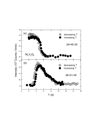
Figure 6: Top: Intensity at the scattering angle $2\Theta$, close to the AF peaks $(1,1,2)$ and $(1,3,0)$. The intensity above $4$K is related to $(0.73,3,1)$ magnetic reflection associated with the incommensurate magnetic structures. Bottom: Intensity at the scattering angle $2\Theta$ for the incommensurate magnetic peak $(0.73,1,0)$ as a function of temperature.

The magnetic order was further investigated with experiments on a single-crystal in which scattering was monitored only in the $(h,k,0)$ and $(h,k,k)$ planes. Fig. 7 shows the elastic neutron scattering at three different temperatures for wavevectors of the form $(Q_{x},1,0)$. Upon entering the magnetic phase, a Bragg peak is formed with a maximum intensity for $Q_{x}=Q_{x}^{0}\approx 1.27$ r. l. u.’s. This result indicates weight in the Fourier transform of the spin $S({\bf Q})$ at a wavevector $(Q_{x}^{0},1,0)$ which is outside the first Brillouin zone of the primitive unit cell. We deduce that, Bragg scattering is allowed at wavevectors

$${\bf G}+{\bf q}\equiv{\bf G}\pm(q,0,0)\ ,$$ (16)

where $q\approx 0.27$ and ${\bf G}$ is a reciprocal lattice vector of the form $G=(l+m,l-m,n)$, where $l$, $m$, and $n$ are integers. The ordering wave-vector in the HTI and LTI phases is thus ${\bf v}=(q,0,0)$. The peak in Fig. 7 is in the $l=1,m=n=0$ zone. In this formulation the wavevector ${\bf q}$ indicates that the spin function varies as $\exp(i{\bf q}\cdot{\bf R})$ as the position is displaced through a translation vector ${\bf R}$ of the lattice, as defined in the caption to Fig. 4. Thus, for a given irrep, the actual spin amplitudes are determined by the value of $q$ and the value of the spin coordinates within the unit cell as given in Table 7 (or 8).

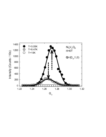
Figure 7: Neutron diffraction intensity measured as a function of $Q_{x}$ for wavevector ${\bf Q}$=$(Q_{x},1,0)$. Here the peak position determines the value of $1+q$.

Note that this wavevector $q$ does NOT give the phase factor introduced upon moving from one spine site to its nearest neighbor. In view of the intra-cell structure (given in Table 7), different components of spin will involve different phase factors. If we consider the ${\bf a}$-component of spin in irrep $\Gamma_{4}$ and let the translation vector ${\bf R}$ be $(X,Y,Z)$, then we see that

$$S_{s1,a}(X) = e^{iq(2\pi/a)[X+(a/4)]}m_{s}^{a}\ ,$$

$$S_{s4,a}(X) = e^{iq(2\pi/a)[X+(3a/4)]}(-m_{s}^{a})\ ,$$ (17)

where $s1$ and $s4$ are site labels as in Fig. 4. Thus $S_{s4,a}(X)/S_{s1,a}(X)=-e^{iq\pi}$. Similarly one finds $S_{s1,a}(X+a)/S_{s4,a}(X)=-e^{iq\pi}$. Our conclusion is that translation along a spine by $a/2$ introduces a phase factor $e^{i(q+1)\pi}$. So, the wavevectors for the $a$-component along a single spine are $q_{\pm}=1\pm q$. As we shall see later, other wave-vectors are needed to reproduce the position dependence of other spin components within this representation.

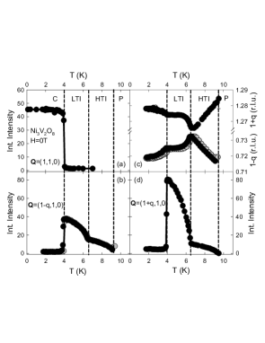
Figure 8: Temperature dependence of magnetic Bragg peaks in zero field. The low-temperature field was reached by zero-field cooling. Integrated intensities were obtained by integrating diffraction intensities measured as a function of $h$ wave-vector transfer. (a) Temperature dependence of $h$-integrated intensity of the AF $(1,1,0)$ reflection. (b) Temperature dependence of $h$-integrated intensity of the incommensurate $(1-q,1,0)$ reflection. (c) Temperature dependence of the wave-vector $(1\pm q,1,0)$ of the incommensurate magnetic reflections. (The data points below $T=4$K represent nonequilibrium domains of the LTI phase embedded in the C phase. Such peaks are only present after cooling through the LTI phase.) (d) Temperature dependence of $h$-integrated intensity of the incommensurate $(1+q,1,0)$ reflection.

The incommensuration $q$ is weakly temperature dependent, as shown in Fig. 8c, indicating competing interactions in the spin lattice. The temperature dependence of the integrated intensity of the incommensurate Bragg peaks indicates the onset of magnetic order at $T_{\rm PH}=9.1$K and further a second order transition at about $T_{\rm HL}=6.3$K. These transition temperatures are consistent with specific heat measurements, which show sharp peaks at these temperatures, and with magnetization data. The existence of two different incommensurate magnetic phases is a further indication of competing interactions in NVO.

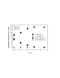
Figure 9: Integrated intensity of the $(1,1,0)$ and the $(0.72,1,0)$ reflections for increasing and decreasing field after the sample was cooled in zero field.

Fig. 8 shows that the incommensurate Bragg peaks abruptly lose most of their intensity at $T_{\rm LC}=4$K, below which temperature a commensurate magnetic order becomes dominant. Commensurate Bragg peaks were observed at the $(h,k,0)$ for $h+k=$ even, so the commensurate structure is associated with an ordering wave-vector ${\bf v}=(0,0,0)$. The magnetic unit cell in the C phase is thus identical to the chemical unit cell.

In the zero-field cooled sample, we observed a weak incommensurate peak which is not present in the $8$T field cooled sample. This is evidence that the incommensurate phase below $T_{\rm LC}$ is metastable - possibly a reflection of how close the commensurate and incommensurate magnetic order lie in energy. However, Fig. 9 shows that the ground state of NVO can be annealed through the application of a field along the c-axis which makes the incommensurate Bragg peak vanish. The incommensurate Bragg peaks do not reappear when lowering the field, but the intensity is instead transferred to the commensurate peak that grows in strength.

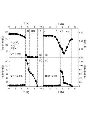
Figure 10: Temperature dependence of magnetic Bragg peaks for $H=2$T, applied along the crystallographic c-axis. The low-temperature state was reached by cooling the sample in a field of $8$T. Integrated intensities were obtained by integrating the intensity of the magnetic Bragg reflection when opbserved by a scan over the $h$-component of the wave-vector transfer. (a) Temperature dependence of integrated intensity of the AF $(1,1,0)$ reflection. (b) Temperature dependence of integrated intensity of the incommensurate $(1-q,1,0)$ reflection. (c) Temperature dependence of the incommensuration $q$. (d) Temperature dependence of integrated intensity of the incommensurate $(1+q,1,0)$ reflection.

IV.4 Field dependence of Bragg reflections

The field dependence of the magnetic Bragg reflections was investigated only with fields along the c-axis. Fig. 10 shows the magnetic reflections at $2$T as a function of temperature. Upon heating, the $(1,1,0)$ reflection disappears in a first-order transition as the incommensurate $(1\pm q,1,0)$ reflections appear. The commensurate phase survives to higher temperatures than at zero field, and the ordered moment increases with field, both indications that the magnetic field stabilizes the commensurate order. The LTI magnetic structure occupies a relatively narrow temperature range while the temperature boundaries for the HTI magnetic structure are nearly independent of field.

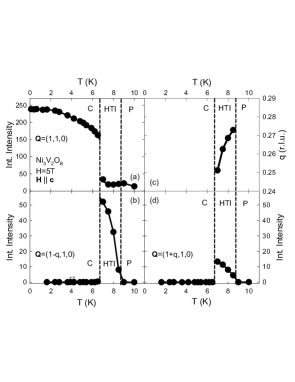
Figure 11: As for Fig. 10, but for $H=5$T.

The LTI magnetic structure is further suppressed with increasing magnetic field along the c-axis. At $5$T, as shown in Fig. 11, the LTI structure does not occur, and as the temperature is increased, the commensurate structure gives way directly to the HTI magnetic structure. The phase transition between the paramagnetic and HTI phase occurs at a temperature somewhat below its zero-field critical temperature $T_{\rm PH}=9$K. It is for this field direction that the phase boundaries depend most strongly on the field. The magnetic phase boundaries obtained with these neutron measurements are consistent with the phase diagram obtained through specific heat measurement with the field along the c-axis.

A field along the ${\bf c}$ axis in the HTI phase leads to suppression of the incommensurate Bragg peak at $(1-q,1,0)$ and an increase in the intensity of the $(1,1,0)$ reflection, as shown in Fig. 12 for $T=8.4$K. The temperature dependence of the intensity of the incommensurate Bragg peaks suggests that the HTI phase disappears in a continuous phase transition at a critical field $H_{c}$, giving way to a commensurate field driven AF phase at higher fields. This contrasts with the first order nature of the phase boundary between the LTI and AF phases. As shown in Fig. 12, both the incommensurate wave vector, $q$, and the integrated intensity of the (1,1,0) AF Bragg peak increase progressively more rapidly as the field increases.

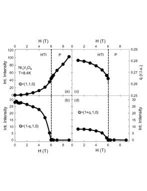
Figure 12: Field dependence of magnetic Bragg peaks at $T=8.4$K. Integrated intensities were obtained as for Fig. 10. Field dependence of the integrated intensity of (a) the AF $(1,1,0)$ reflection, (b) the incommensurate $(1-q,1,0)$ reflection and (d) the incommensurate $(1+q,1,0)$ reflection. (c) shows the field dependence of the incommensurate wave vector $q$.

IV.5 Phase diagram

The zero-field phase boundaries at $T_{\rm PH}$, $T_{\rm HL}$ and $T_{\rm LC}$ deduced from the diffraction experiments are consistent with those observed with specific heat measurements. In contrast, the intensity of the $(1,1,0)$ does not show any anomaly at $T_{\rm CC^{\prime}}$, to a level of $0.5\%$. This suggests that the CC’ phase transition leaves the magnetic structure of C-phase described by ordering wave-vector ${\bf v}=(0,0,0)$ unaltered.

Figures 10 and 11 already show that the C-LTI and the C-HTI transitions are first order at small $H$. Similar results were obtained when we varied $H$ at fixed $T$. Specifically, Fig. 14 shows the jumps in the staggered moment of the C phase as one moves from the LTI or from the HTI phases into the C phase, for $T<8$K. In contrast, at higher temperatures and fields the transition from the HTI to the P phase is continuous, as can be seen from Fig. 12. In fact, at finite field along ${\bf c}$ one cannot really distinguish between the P and the C phases, and we already saw in Figs. 10 and 11 that the HTI-P transition is continuous for $H\leq 5$T. We thus conclude that the HTI-C transition changes from being continuous to being first order somewhere around the top of the boundary of the HTI phase in Fig. 1. Such tricritical points are abundant in anisotropic antiferromagnets subject to magnetic fields.

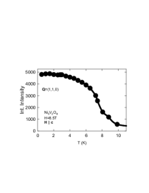
Figure 13: Temperature dependence of $h$-integrated intensity of the AF $(1,1,0)$ reflection in a field of $H=8.5$T, applied along the c-axis, showing the absence of a second order phase transition when cooling from the paramagnetic phase to the low-temperature commensurate phase. The data instead reflect a cross over phenomenon for $T\approx 8$K.

The change in slope of the $(110)$ intensity versus $T$ curve at the HTI-P transition (see Fig. 12) indicates the coupling between the commensurate and incommensurate order parameters, which will be discussed in Sec. V.4.

The observations which are relevant for the C phase are (a) the specific heat data at 9T which show no anomaly and (b) the lack of any detectable anomaly in the $T$-dependence of the(110) peak intensity (see Fig. 13). As will be shown in Sec. V.3.1, the P phase in a field allows the development of order characteristic of only the irrep $\Gamma_{7}$ in which there is a uniform moment along ${\bf c}$ and a staggered moment along a. This suggests that the magnetic structure in the C and P phase (in a field) exhibit the same symmetry, and that the symmetry at high field at low and high temperature is the same as that of the C phase at zero field because it can be reached without crossing a second order phase transition.

IV.6 Magnetic Structures

Even more detailed information about the spin interactions can be obtained by determining the symmetry of the ordered magnetic structures. In this paper, we will focus our attention on the HTI, LTI, C and P phases, and we will leave a discussion of the C’ phase for a later publication.

IV.6.1 High-temperature incommensurate (HTI) structure

For temperatures between $T_{\rm HL}$ and $T_{\rm PH}$, Bragg reflections occur at the $(2n+1\pm q,2m+1,0)$ and $(2n+1\pm q,2m+1,2m+1)$ positions. The intensities of $170$ magnetic Bragg reflections were measured and can be explained with a magnetic structure belonging to representation $\Gamma_{4}$ given in Table 8. The magnetic structure at $T=7$K is given by

$$\tilde{\bf m}_{s}^{\rm\Gamma_{4}} = (1.9(1),0.2(1),0.2(2))\;\mu_{B}$$

$$\tilde{\bf m}_{c}^{\rm\Gamma_{4}} = (0,0.0(1),0.2(2))\;\mu_{B}\ ,$$ (18)

where the number in parenthesis is the uncertainty in the last digit quoted. The quality of the fit is given by $R_{\rm p}$=$0.15$ and $\chi^{2}$=$12$ (see Table 1 for the definition of these quantities). The spin arrangement at $T=7$K is illustrated in Fig. 15b. It is predominantly a modulated structure on the spine sites with moments that are parallel to the a direction. The moments on the cross-tie sites either vanish or are very small. [If the cross-tie moments in the b direction are nonzero, they are out of phase with the spine moments because of the phase factor introduced by Eq. (11)].

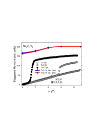
Figure 14: Field dependence of effective staggered moment at three different temperatures, obtained from the $(1,1,0)$ reflection by taking the square root of the peak intensity.

To determine the HTI magnetic structure in a magnetic field along the c-axis, we measured the intensity of $28$ magnetic Bragg peaks in the $(h,k,0)$ plane for $T$=$8$K and $H$=$5$T. The data is best described by the basis vectors of the irrep $\Gamma_{4}$, and the magnetic structure is given by

$$\tilde{m}_{s}^{\Gamma_{4}} = (1.60(4),0.08(3),0(2))\mu_{B}$$

$$\tilde{m}_{c}^{\Gamma_{4}} = (0,0.02(5),0(2))\mu_{B}$$ (19)

The quality of the fit is given by $R_{\rm p}$=$0.14$ and $\chi^{2}$=$6.7$. The effect of the field along the c-axis is thus to reduce the ordered moment along the a-axis compared to the zero-field structure at a somewhat lower temperature. This may be because the field induces a uniform moment along the c-axis which reduces the amount of moment available along the a-axis.

IV.6.2 Low-temperature incommensurate (LTI) structure

For temperatures between $T_{\rm LC}$ and $T_{\rm HL}$, Bragg reflections were observed at the $(2n+1\pm q,2m+1,0)$ and $(2n+1\pm q,2m+1,2m+1)$ positions. These are the same Bragg peaks as observed in the HTI phase, but their relative intensity has changed, indicating that the spins undergo a spin reorientation at $T_{\rm HL}$. The present diffraction data are consistent with either a $\Gamma_{1}+\Gamma_{4}$ or a $\Gamma_{2}+\Gamma_{4}$ structure. We choose the former spin structure, not because it has a smaller value of $\chi^{2}$, but because it is consistent with the appearance of ferroelectricity, as is discussed in Sec. IV.7, below. With that assumption the magnetic structure at $5$K is given by

$$\tilde{\bf m}_{s}^{\rm\Gamma_{4}} = (1.6(1),0.03(10),0.01(7))\;\mu_{B}$$

$$\tilde{\bf m}_{s}^{\rm\Gamma_{1}} = (0.0(5),1.3(1),0.1(1))\;\mu_{B}$$

$$\tilde{\bf m}_{c}^{\rm\Gamma_{4}} = (0,1.4(1),-0.04(9))\;\mu_{B}$$

$$\tilde{\bf m}_{c}^{\rm\Gamma_{1}} = (-2.2(1),0,0)\;\mu_{B}\,.$$ (20)

The quality of the fit is given by $R_{\rm p}$=$0.19$ and $\chi^{2}$=$7$. The corresponding spin structure is shown in Fig. 15c and consists of elliptical ${\bf a}-{\bf b}$ plane spirals on spine and cross-tie sites.

The structure at $T=5$K thus consists of spirals on the spine and cross-tie sites, propagating along the a-axis with moments in the a-b-plane, as shown in Fig. 15d. An inspection of the spin structure suggests that nn interactions between Ni on adjacent spines are AF, both within and between Kagomé planes. The moment in the c-direction is zero within the error bar, indicating the presence of a spin anisotropy which forces the spin into the ab plane.

To determine the LTI magnetic structure in a magnetic field along the c-axis, we measured the intensity of $28$ magnetic Bragg peaks in the $(h,k,0)$ plane for $T$=$6$K and $H$=$2$T. We obtained best agreement with the experimental data for basis vectors belonging to the irreps $\Gamma_{1}$ and $\Gamma_{4}$. The structure is given by

$$\tilde{\bf m}_{s}^{\rm\Gamma_{4}} = (2.5(1),-0.1(2),0(2))\;\mu_{B}$$

$$\tilde{\bf m}_{s}^{\rm\Gamma_{1}} = (-0.5(3),1.1(1),0(2))\;\mu_{B}$$

$$\tilde{\bf m}_{c}^{\rm\Gamma_{4}} = (0,0.0(1),0(2))\;\mu_{B}$$

$$\tilde{\bf m}_{c}^{\rm\Gamma_{1}} = (0.06(8),0,0)\;\mu_{B}\,,$$ (21)

The quality of the fit is given by $R_{\rm p}$=$0.29$ and $\chi^{2}$=$9.3$. Qualitatively, these parameters are similar to those of the zero-field structure. We remind the reader that Eq. (11) implies a phase difference of $\pi/2$ between the ${\bf a}$- and ${\bf b}$-components on the spine sites. The high-field LTI phase thus consists of a spiral on the spine sites and no moment on the cross-ties, possibly because a transverse field has a strong effect on the cross-ties which are more weakly coupled antiferromagnetically. In contrast to the HTI phase, however, the ordered moment at non-zero field is higher moment than at zero field.

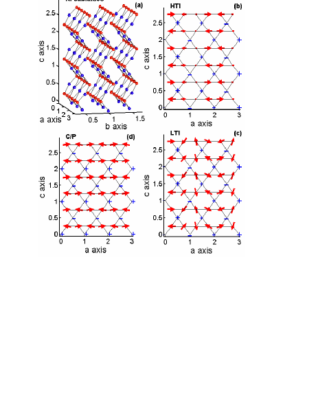
Figure 15: Lattice (a) and magnetic structure (b-d) of various phases. The size of the $+$ and $-$ signs correspond to the components out of the page and into the page, respectively. In panel (d) the canting of the C phase is magnified for legibility. For the HTI and LTI phases, the ${\bf a}$-component has a wavelength approximately $1.4a$ so that $q\approx 0.27$, as indicated in Fig. 7.

IV.6.3 P and C phase

The C phase has the same symmetry as the P phase, and for fields along the c-axis, there is no phase boundary between the high-field phase and the zero-field phase for $T_{\rm CC^{\prime}}<T<T_{\rm LC}$. The symmetry of the C magnetic structure can thus be determined in a high magnetic field along the c-axis. We measured a set of magnetic Bragg peaks in the $(h,k,0)$ plane at $T=0.1$K and $H=8$T, and we found that the data is best described by irrep $\Gamma_{7}$ and the parameters

$${\bf m}_{s}^{\rm\Gamma_{7}} = (2.4(1),0,0.0(5))\;\mu_{B}$$

$${\bf m}_{c}^{\rm\Gamma_{7}} = (0,0.8(1),0(1))\;\mu_{B}\,.$$ (22)

The quality of the fit is given by $R_{\rm p}$=$0.23$ and $\chi^{2}$=$17$. When we allowed the fit to include also $\Gamma_{1}$ parameters, the components of the magnetization were found to be $0.1(1)\mu_{B}$ and therefore statistically insignificant.

A magnetic field along the c-axis induces magnetic order even in the paramagnetic phase. At $T=10$K and $H=8$T, the spin structure is best described by the irrep $\Gamma_{7}$ with the following parameters:

$${\bf m}_{s}^{\rm\Gamma_{7}} = (0.61(2),0,0.0(2))\;\mu_{B}$$

$${\bf m}_{c}^{\rm\Gamma_{7}} = (0,0.37(3),0.0(4))\;\mu_{B}\,.$$ (23)

The quality of the fit is given by $R_{\rm p}$=$0.31$ and $\chi^{2}$=$2.49$. Thus the field-induced magnetic structure at $T=10$K is described by the same irrep as at $T=0.1$K and $H=8$T. This is corroborated by the absence of a phase transition upon cooling in a high field, as shown in the temperature dependence of the $(1,1,0)$ Bragg peak shown in Fig. 13.

IV.7 Ferroelectricity

Recently NVO has been shown to have remarkable ferroelectric behavior.FERRO A spontaneous polarization ${\bf P}$ has been found to appear only in the LTI phase. In other words, upon cooling into the LTI phase, the ferroelectric order parameter develops simultaneously with the LTI magnetic order parameter. In Ref. FERRO, it was proposed that the multi-component order parameter associated with this phase transition requires the trilinear coupling, $V$, where

$$V = \sum_{\gamma}\Biggl{[}a_{\gamma}\sigma_{\rm LTI}^{*}\sigma_{\rm HTI}+a_{\gamma}^{*}\sigma_{\rm LTI}\sigma_{\rm HTI}^{*}\Biggr{]}P_{\gamma}\ .$$ (24)

Here $P_{\gamma}$ is the $\gamma$-component of the spontaneous polarization and the $\sigma$’s are complex-valued order parameters which describe the incommensurate long range order associated with irrep $\Gamma_{4}$ for the HTI phase and with irrep $\Gamma_{1}$ for the additional order parameter appearing in the LTI phase. Of course, $V$ must be invariant under the symmetry operations of the paramagnetic phase.IED ; LL As we have seen, the magnetic order parameters satisfy Eq. (8), which here is

$${\cal I}\sigma_{\rm A} = \sigma_{\rm A}^{*}\ ,$$ (25)

where A denotes either LTI or HTI. Using this relation, we see that the invariance of $V$ under spatial inversion implies that $a_{\gamma}$ is pure imaginary: $a_{\gamma}=ir_{\gamma}$, where $r_{\gamma}$ is real valued. Thus we may write

$$V = 2\sum_{\gamma}r_{\gamma}P_{\gamma}|\sigma_{\rm LTI}\sigma_{\rm HTI}|\sin(\phi_{\rm HTI}-\phi_{\rm LTI})\ ,$$ (26)

where the phases are defined by $\sigma_{\rm A}=|\sigma_{\rm A}|e^{i\phi_{\rm A}}$.

To be invariant under the operations of the little group $P_{\gamma}$ must transform like $\Gamma_{4}\otimes\Gamma_{1}$. Referring to Table 6, we see that this means that $P_{\gamma}$ has to be odd under $2_{a}$ and $m_{ac}$. The first of these conditions means that $r_{\gamma}$ can only be nonzero for $\gamma=b$ or $\gamma=c$. The second condition means that $r_{\gamma}$ can only be nonzero for $\gamma=b$, in agreement with the observationFERRO that the spontaneous polarization only appears along the b-direction. Had we chosen the irrep $\Gamma_{2}$ for the new LTI representation in Eq. (20), we would have incorrectly predicted the spontaneous polarization to be along the ${\bf c}$-direction.

IV.8 Magnetization and Susceptibility Measurements

Although neutron diffraction enables one to fix many details of the magnetic structure, it is hard to obtain the bulk magnetization from these measurements because the signal associated with bulk magnetization is buried in the nuclear Bragg peaks. Accordingly, we summarize here the results for the zero wavevector magnetization, $M$, measured with a SQUID magnetometer, as a function of field for fields along each of the crystallographic directions shown in Figs. 16 and 17.

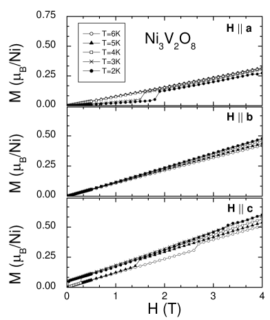
Figure 16: $M$ versus $H$ along the three crystallographic axes for a sequence of temperatures.

The following features are noteworthy. In Fig. 16 one sees that for $H$ along the c-axis, there is a range of temperature (corresponding to the C phases) in which $M$ vs $H$ does not extrapolate to zero for $H\rightarrow 0$. This is the best measurement of the weak FM moment in this phase. The C’ phase may also have a finite remnant magnetization though further measurements are needed there. From these data one sees confirmation of the phase boundaries obtained from specific heat measurements (shown in Fig. 1) which here are signaled by discontinuities in the magnetization as a function of $H$ (when a phase boundary is crossed.) In Fig. 17 we show $M/H$, measured for a small field $H=0.1$T. This quantity will be nearly equal to the zero field susceptibility except when it probes the spontaneous magnetization, as when ${\bf H}$ is along (0,0,1) and $T<4$K and the system is in the C or C’ phase. It is remarkable that there are no visible anomalies associated with the phase transitions involving the HTI phase.

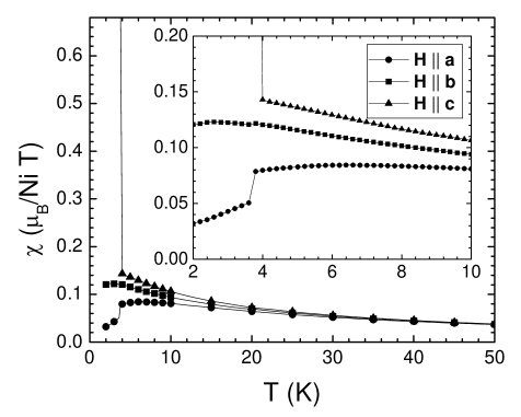
Figure 17: $\chi$ for magnetic field applied along each of the crystallographic directions in Bohr magnetons per Ni ion per Tesla versus $T$, where $\chi$ is defined by $\chi=M(H=0.1$T$)/H$.

V Theoretical Interpretations

Here we discuss the simplest or “minimal” model that can explain the experimental results for NVO. In general, the higher the temperature the simpler the model needed to explain experimental results. Accordingly, we discuss the theoretical models for the phases in the order of decreasing temperature. That way, we will see that the minimal model is constructed by sequentially including more terms as lower temperature phases are considered.

V.1 The high temperature incommensurate (HTI) phase

V.1.1 Competing nearest and next nearest neighbor interactions

Incommensurate phases usually result from competing interactions. In the HTI phase we found spin ordering predominantly on the spine sites [see Eq. (18)], so the minimal model will deal only with the spine spins. Since the incommensurate wave vector is along the spine axis, it is reasonable to infer that this incommensurability arises from competition between nn and nnn interactions along a spine. We already indicated that such competition is plausible, in view of the nearly 90^o angle of the nn Ni-O-Ni bonds. Thus the minimal model to describe the incommensurate phase is

$${\cal H}_{\rm spine} = {1\over 2}\sum_{n=1}^{2}\sum_{\alpha}J_{n\alpha}\sum_{{\bf r},\delta_{n}}S_{\alpha}({\bf r})S_{\alpha}({\bf r}+\delta_{n})$$ (27)

$$+ {\cal H}_{\rm A}+{\cal H}_{ss^{\prime}}\ ,$$

where $J_{1\alpha}$ and $J_{2\alpha}$ represent the (a priori anisotropic) nn and nnn exchange interactions, $\alpha$ is summed over the axes $a,~{}b$ and $c$, ${\bf r}$ is summed over only spine sites, and $\delta_{n}=\pm(n/2)a\hat{\bf a}$ are the first and second neighbor displacement vectors for the spine sites (remember that there are two spine spins along each spine axis in the unit cell, so the nn distance is $a/2$). Also ${\cal H}_{ss^{\prime}}$ represents (probably weak) AF interactions between nn in adjacent spines: $J_{b\alpha}$ for spins at a distance $b/2$ in the b-direction and $J_{c\alpha}$ for spins at a distance $c/2$ in the c-direction. (In this minimal model, for the purpose of Fourier transformation, we place the lattice sites on an orthorhombic lattice for which the ${\bf a}-{\bf c}$ planes are not buckled, but we retain the same interactions between spins as for the buckled lattice. In this way our model gives the correct thermodynamics, even though it should not be used to obtain scattering intensities.)

To have competition, we must have $J_{2\alpha}>0$ (at least for the relevant $\alpha$, which turns out to be $\alpha=a$). Given that at low temperature we end up with a commensurate AF ordering of the a-spin components, it is also reasonable to assume that $J_{1\alpha}>0$ (at least for $\alpha=a$). If the spines did not interact with one another, they would form an array of independent one-dimensional systems for which thermal and/or quantum fluctuations would destroy long-range order. To understand the coupling between adjacent spines, note that a displacement $({\bf b}/2)$ (from a spine in one Kagomé layer to a spine in an adjacent Kagomé layer) takes site #1 in one unit cell into site #4 in another unit cell and vice versa. Similarly this displacement takes site #2 in one unit cell into site #3 in another unit cell and vice versa. From Table VII (or VIII) one see that for the active irreps #4 and #1 such a nearest neighbor displacement along ${\bf b}$ corresponds to a change in the signs of $m_{sa}$ and $m_{sb}$. The fact that these are the dominant order parameters for the spine sites therefore strongly suggests that the nn interspine interactions along ${\bf b}$ are antiferromagnetic. The evidence for antiferromagnetic interactions along ${\bf c}$ is almost as compelling. For these nn pairs (sites #1 and #2, or sites #3 and #4) the largest order parameters of the LTI phase (see Eq. (20))B, i. e. the $x$ components of spine spins ordered according to irrep #4 and the $y$ component ordered according to irrep #1 are both antiferromagnetic along ${\bf c}$. While it is true that the ordering of the $x$-component according to irrep #1 is ferromagnetic along ${\bf c}$, this component of the order parameter is indistinguishable from zero. Thus we conclude that the nn interactions $J_{1\alpha}$ for all directions $\alpha$ are antiferromagnetic.

Also, in Eq. (27) ${\cal H}_{\rm A}$ is a single ion anisotropy,

$${\cal H}_{A}=-\sum_{\alpha}A_{\alpha}\sum_{\bf r}S_{\alpha}({\bf r})^{2}\ .$$ (28)

The continuum mean-field phase diagram of this Hamiltonian is known, for both exchange and single ion anisotropies.Nagamiya ; Kaplan To determine which phase orders as the temperature is lowered from the paramagnetic phase, it is sufficient to look at the quadratic terms in the expansion of the free energy per spin in the Fourier components of the spins,

$$F^{\rm spine}_{2}={1\over 2}\sum_{\bf p}\sum_{\alpha}[\chi_{s,\alpha}({\bf p})]^{-1}S_{\alpha}({\bf p})S_{\alpha}(-{\bf p})\ ,$$ (29)

where

$$[\chi_{s,\alpha}({\bf p})]^{-1}=T/C+{\hat{J}}_{\alpha}({\bf p})-2A_{\alpha}$$ (30)

is the $\alpha$-component of the inverse susceptibility of the spine sites associated with the Fourier component

$$S_{\alpha}({\bf p})=\sum_{\bf r}S_{\alpha}({\bf r})e^{-i{\bf p}\cdot{\bf r}}/{\cal N}$$ (31)

(with the sum over all the ${\cal N}=4N_{uc}$ spine spins in the lattice), while ${\hat{J}}_{\alpha}({\bf p})$ is the Fourier transform of the exchange interactions. In Eq. (30), $C$ is the Curie constant,

$$C=S(S+1)/3=2/3.$$ (32)

(We measure energy in temperature units, which amounts to setting the Boltzmann constant $k=1$.) For our simple model (27),

$${\hat{J}}_{\alpha}({\bf p}) = 2[J_{1\alpha}\cos(p_{a}a/2)+J_{2\alpha}\cos(p_{a}a)$$ (33)

$$+ J_{b\alpha}\cos(p_{b}b/2)+J_{c\alpha}\cos(p_{c}c/2)]\ .$$

As $T$ is lowered, the first phase to order will involve the order parameter $S_{\alpha}({\bf p})$ for which $[\chi_{s,\alpha}({\bf p})]^{-1}$ first vanishes. For $J_{1\alpha}>4|J_{2\alpha}|$, this happens for

$${\bf p}={\bf Q}_{0}\equiv 2\pi(1/a,1/b,1/c),$$ (34)

implying a simple two sublattice antiferromagnet along each spine chain (with the orthorhombic unit cell containing four spins in each sublattice, and with the spins inside the unit cell varying with $e^{i{\bf Q}_{0}\cdot{\bf r}}$). However, for $J_{2\alpha}>|J_{1\alpha}|/4$, the minimum in ${\hat{J}}_{\alpha}({\bf p})$ occurs at the incommensurate wave vector

$${\bf p}_{0\alpha}=2\pi(q_{0\alpha}/a,1/b,1/c).$$ (35)

The modulation wave vector $q_{0\alpha}$ for the $\alpha$ spin component (in r.l.u.’s) is given by

$$\cos(\pi q_{0\alpha}) = -J_{1\alpha}/(4J_{2\alpha})\ ,$$ (36)

and thus the susceptibility for this wavevector becomes

$$[\chi_{s,\alpha}({\bf p}_{0\alpha})]^{-1} = T/C-2[J_{2\alpha}+J_{1\alpha}^{2}/(8J_{2\alpha})$$ (37)

$$+ J_{b\alpha}+J_{c\alpha}+A_{\alpha}].$$

Experimentally, we know that the leading order parameter in the HTI phase concerns $S_{a}({\bf p}_{0a})$. In this phase, the neutron diffraction data also give a wave vector which varies slightly with temperature, close to $q_{0a}=1\pm q\approx 0.72$ or 1.28. To avoid confusion, from now on we use the notation $q_{0}=0.72$. Using this approximate value, Eq.  (36) gives

$$J_{1a}\approx 2.55J_{2a}.$$ (38)

Thus we conclude that at this mean field level one has

$$T_{\rm PH}=2C[J_{2a}+J_{1a}^{2}/(8J_{2a})+J_{ba}+J_{ca}+A_{a}],$$ (39)

and we end up with a longitudinally modulated spin structure, with $S_{b}({\bf r})=S_{c}({\bf r})=0$ and, along a single spine,

$$S_{a}(x)=S\cos(2\pi q_{0}x/a+\phi_{n}),$$ (40)

where the phase $\phi_{n}$ may depend on the spine index $n$. The $n$-dependence of $\phi_{n}$ would be determined by the inter-spine coupling. For our model the neutron diffraction data indicates that adjacent spines are antiferromagnetically arranged, so that for a general spine site we may write

$$S_{a}({\bf r})=S\cos({\bf p}_{0}\cdot{\bf r}+\phi_{0})\ ,$$ (41)

where the transverse components of ${\bf p}_{0}$ are fixed as in Eq. (35) and we adopt the notation ${\bf p}_{0}\equiv{\bf p}_{0a}$. When one goes beyond continuum mean-field theory, it is found that instead of $q_{0}$ being a continuous function of $J_{1a}$ and $J_{2a}$ one obtains a ‘devil’s staircase’ dependence of the wave vector on the control parameters.Aubry ; ANNNI This treatment also shows that $\phi_{0}$ can not be fixed arbitrarily (as it would be in continuum mean-field theory). Furthermore, critical fluctuations will reduce the actual $T_{\rm PH}$ by a factor which depends on the spatial anisotropy.

V.1.2 Dzyaloshinskii-Moriya interactions

In addition to the leading a-component of the spine spins, Eq. (18) also indicates a small, but non-negligible, spine moments along the b-axis and along the c-axis. Such moments follow directly from the Dzyaloshinskii-Moriya (DM) interactionsDzyaloshinskii ; Moriya between spine spins. For simplicity, we consider here only the nn DM interactions along the spine,

$${\cal H}_{DM}=\sum_{\bf r}{\bf D}({\bf r})\cdot{\bf S}({\bf r})\times{\bf S}({\bf r}+a{\hat{\bf a}}/2),$$ (42)

and the symmetry of the lattice dictates that the DM vectors behave as

$${\bf D}({\bf r})=\bigl{(}0,D_{b}e^{i{\bf Q}_{0}\cdot{\bf r}},D_{c}e^{i{\bf P}_{c}\cdot{\bf r}}\bigr{)},$$ (43)

where ${\bf Q}_{0}$ is the wave vector for the two-sublattice commensurate wave vector [Eq. (34)], while ${\bf P}_{c}=(0,0,2\pi/c)$ represents AF ordering along the c-axis. Next nearest neighbor DM interactions, discussed in II, do not change the qualitative results presented here. The Fourier representation of ${\cal H}_{DM}$ yields a free energy of the form

$$F_{DM}=\sum_{\bf p}\bigl{[}D_{b}\cos(p_{a}a/2)S_{a}({\bf p})S_{c}(-{\bf p}-{\bf Q}_{0})$$

$$-iD_{c}\sin(p_{a}a/2)[S_{a}({\bf p})S_{b}(-{\bf p}-{\bf P}_{c})]+h.c..$$ (44)

Introducing quadratic terms in the transverse spine spin components, as in Eq. (29), we can now minimize the free energy and find these transverse components: a non-zero $S_{a}({\bf p}_{0})$ generates

$$S_{c}({\bf p}_{0}+{\bf Q}_{0}) \approx -2D_{b}\chi_{s,c}({\bf p}_{0}+{\bf Q}_{0})\cos(\pi q_{0})S_{a}({\bf p}_{0}),$$

$$S_{b}({\bf p}_{0}+{\bf P}_{c}) \approx 2iD_{c}\chi_{s,b}({\bf p}_{0}+{\bf P}_{c})\sin(\pi q_{0})S_{a}({\bf p}_{0}),$$ (45)

consistent with the signs and phases of $\tilde{m}_{s}^{b}$ in Table 8. In fact, for all the group representations, all the internal structure within the orthorhombic unit cell can be reproduced using factors like $e^{i{\bf p}\cdot{\bf r}}$, with the three wave vectors ${\bf p}_{0}$, ${\bf p}_{0}+{\bf Q}_{0}$ and ${\bf p}_{0}+{\bf P}_{c}$ (with possibly different ${\bf p}_{0}$’s for different representations).

Using the values from Eq. (18), and $p_{a}=2\pi q_{0}/a$ with $q_{0}\approx 0.72$, Eq. (45) yields

$$D_{c} \approx -0.07[\chi_{s,b}({\bf p}_{0}+{\bf P}_{c})]^{-1},$$

$$D_{b} \approx 0.04[\chi_{s,c}({\bf p}_{0}+{\bf Q}_{0})]^{-1}.$$ (46)

Near $T_{\rm PH}$ , $[\chi_{s,a}({\bf p}_{0})]^{-1}$ is small, but $[\chi_{s,b}({\bf p}_{0}+{\bf P}_{c})]^{-1}$ and $[\chi_{s,c}({\bf p}_{0}+{\bf Q}_{0})]^{-1}$ remain finite. Since $T_{\rm PH}=9.1$K, it is reasonable to assume that all these inverse susceptibilities are of order 10K. Thus we have the estimates, $D_{b}\sim 0.4$K and $D_{c}\sim-0.7$K. Below we conjecture a set of exchange parameters, which give $[\chi_{b}({\bf p}_{0}+{\bf P}_{c})]^{-1}\sim 13$K and $[\chi_{c}({\bf p}_{0}+{\bf Q}_{0})]^{-1}\sim 47$K, changing these estimates into $D_{b}\sim 0.5$K and $D_{c}\sim-3$K.

V.1.3 The spine-cross-tie interactions

The representation $\Gamma_{4}$ also allows some small incommensurate moments along the b and c axes on the cross-tie sites. Indeed, the experimental values in Eq. (18) also allow for such moments, alas with large error bars. Here we discuss the possible theoretical origin for these moments, namely the anisotropic spin interactions between the spine and the cross-tie spins. In all the phases, the two spine chains which are nearest neighbors to a given row of cross-tie sites in an ${\bf a}-{\bf c}$ plane (in this section we ignore the buckling, which does not affect the present considerations) have antiparallel a-components of spins. Thus even in the incommensurate phases, the isotropic nn spine-cross-tie interaction is frustrated, and one needs to add (symmetric and antisymmetric) anisotropic spine-cross-tie interactions. In the simplest approach, these interactions can be written in terms of an effective internal field produced by the four spine spins ($s1$ to $s4$) surrounding a cross-tie spin $c2$ (see Fig. 4), so that

$${\cal H}_{sc}=-\sum_{\alpha}H^{c}_{\alpha}S^{c}_{\alpha}(c2),$$ (47)

with

$$H^{c}_{\alpha}=\sum_{\beta}\sum_{s1}^{s4}{\cal J}_{\alpha\beta}(i)S_{\beta}(i),$$ (48)

where the matrix ${\cal J}(i)$ (which relates to the coupling between the spins at $si$ and at $c2$) contains both symmetric (pseudo-dipolar, PD) and antisymmetric (DM) off-diagonal terms, whose signs depend on $i$ (see II). Ignoring the interactions among cross-tie spins, each such spin will follow its local field,

$$S_{\alpha}^{c}(c2)=\chi_{c,\alpha}H^{c}_{\alpha},$$ (49)

where $\chi_{c,\alpha}$ is the $\alpha$-component of the cross-tie susceptibility.

The above analysis yields the spin components on each cross-tie site in terms of the four surrounding spine spins. Taking also into account the variation of the matrices ${\cal J}(i)$ for different plaquettes, and assuming only linear response for the cross-tie spins, we end up with

$$S_{c}^{c}({\bf p}_{0}) = -4\chi_{c,c}(j_{ac}-d_{b})S_{a}({\bf p}_{0})\sin(\pi q_{0}/2),$$

$$S_{b}^{c}({\bf p}_{0}+{\bf P}_{c}) = 4\chi_{c,b}(j_{ab}+d_{c})S_{a}({\bf p}_{0})\sin(\pi q_{0}/2)\ ,$$ (50)

where $j_{\alpha\beta}$ and $d_{\gamma}$ are the symmetric (PD) and anti-symmetric (DM) elements of the matrix ${\cal J}(1)$. Using the experimental values of the cross-tie moments from Eq. (18), we end up with

$$(j_{ab}+d_{c})\chi_{c,b} = -0.06\pm 0.06\ ,$$

$$(j_{ac}-d_{b})\chi_{c,c} = 0\pm 0.06\ .$$ (51)

Ignoring the very weak interaction among the cross-tie spins, we can use the free spin Curie susceptibility, $\chi_{c,\alpha}\approx 1/T\sim 0.2/$K, hence $(j_{ab}+d_{c})\approx-0.3(3)$K, $(j_{ac}-d_{b})\approx 0.0(3)$. However, the uncertainties of these estimates are very large.

V.2 The low temperature incommensurate (LTI) phase

Mean-field theoryNagamiya ; Kaplan also indicates that, if the uniaxial anisotropy energy is not too large, then as the temperature is reduced further below $T_{\rm PH}$, a second continuous phase transition occurs at $T_{\rm HL}$, below which transverse modulated order appears, leading to an incommensurate state with elliptical polarization. Again, this seems to be consistent with the experiments: Eq. (20) indicates a growing $b$-component on the spine spins and a growing $a$-component on the cross-tie spins. For simplicity, we again concentrate only on the spine spins. One can understand this transition intuitively by realizing that as the temperature is lowered the fixed length constraint on spins (embodied in the quartic terms in the Landau expansion) becomes progressively more important. Since the experiment indicates transverse ordering in the b-direction [see Eq. (20)], we conclude that the anisotropies still require that $S_{c}({\bf r})=0$, and we write a Landau expansion in both $S_{a}({\bf p})$ and $S_{b}({\bf p})$. A priori, the quadratic terms in $|S_{a}({\bf p})|^{2}$ and in $|S_{b}({\bf p})|^{2}$ could have minima at slightly different wave vectors ${\bf p}_{1}$ and ${\bf p}_{2}$ respectively [see Eq. (36)]. The quartic coupling between the two spin components would then be of the form $|S_{a}({\bf p}_{1})|^{2}|S_{b}({\bf p}_{2})|^{2}$. Depending on the ratio of the amplitude of this term to those of $|S_{a}({\bf p}_{1})|^{4}$ and $|S_{b}({\bf p}_{2})|^{4}$, one could end up with a second transition, at $T_{\rm HL}<T_{\rm PH}$, at which $S_{b}({\bf p}_{2})$ would begin to order (this is similar to the usual appearance of a tetracritical point, see e.g. Ref. TCP, ). However, the quartic terms also contain a term of the form $[S_{a}({\bf p}_{1})^{2}S_{b}(-{\bf p}_{2})^{2}+h.c.]\delta({\bf p}_{1}-{\bf p}_{2})\equiv 2|S_{a}({\bf p}_{1})|^{2}|S_{b}({\bf p}_{2})|^{2}\cos[2(\phi_{a}-\phi_{b})]\delta({\bf p}_{1}-{\bf p}_{2})$, where we have written $S_{\alpha}({\bf p})=|S_{\alpha}({\bf p})|e^{i\phi_{\alpha}}$. Usually, the coefficient in front of this term is positive, and therefore it is minimized when $\cos[2(\phi_{a}-\phi_{b})]=-1$, and it lowers the free energy only if ${\bf p}_{1}={\bf p}_{2}$. If the values of ${\bf p}_{1}$ and ${\bf p}_{2}$ are sufficiently close to one another, then the presence of this term results in locking the wave vectors to each other: ${\bf p}_{1}={\bf p}_{2}={\bf p}_{0}$, consistent with the experiment.

Thus, within this theory we expect spin ordering of the type

$$S_{a}({\bf r})={\tilde{S}}_{a}\cos({\bf p}_{0}\cdot{\bf r}+\phi_{a}),$$

$$S_{b}({\bf r})={\tilde{S}}_{b}\cos({\bf p}_{0}\cdot{\bf r}+\phi_{b})\,,$$ (52)

with ${\tilde{S}}_{b}$ growing continuously from zero as the temperature is lowered through $T_{\rm HL}$, and with $2(\phi_{a}-\phi_{b})$ an odd integer multiple of $\pi$. The fact that the two order parameters are out of phase can be understood intuitively: if longitudinal and transverse spin components are combined, they are closer to obeying the fixed length constraint if they are out of phase with one another.

Within the Landau theory, we would expect $|{\tilde{S}}_{a}|^{2}$ to grow at $(T_{\rm PH}-T)$ down to $T_{\rm HL}$. Below that temperature, $|{\tilde{S}}_{b}|^{2}$ grows linearly with $(T_{\rm HL}-T)$, while the slope of $|{\tilde{S}}_{a}|^{2}$ versus $T$ decreases. TCP Qualitatively, this is what one observes in Figs. 8, 10 and 11.

The above theory ignores higher harmonics of the incommensurate order parameters. Although these harmonics may be negligible close to $T_{\rm PH}$, they may grow at lower temperatures. Therefore, we went beyond the Landau expansion and numerically minimized the mean field moments on long chains of spin-1 ions with the interaction (27), with an isotropic exchange which has $J_{1}=2.55J_{2}$ and with a uniaxial single-ion energy $A_{a}=K$ (see II for details). The resulting phase diagram, shown in Fig. 18, is qualitatively consistent with the above picture. It is intuitively clear that the range in temperature over which the LTI phase is stable decreases as the anisotropy is increased. (Large anisotropy disfavors the existence of transverse spin components.)

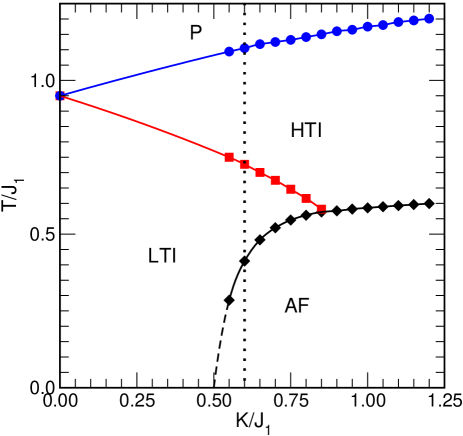
Figure 18: Mean-field phase diagram for the isotropic $J_{1}$-$J_{2}$ model with easy-axis anisotropy scaled by $K\equiv A_{a}$. Here “HTI” denotes a longitudinally polarized incommensurate phase and “LTI” an elliptically polarized incommensurate phase. In both phases the modulation vector is given by Eq. (36). “AF” denotes a two-sublattice collinear AF phase. For large anisotropy this model reduces to the ANNNI model.ANNNI

Having derived the leading order parameter, we can now evaluate secondary spin components, arising due to either the spine-spine DM interaction or the spine-cross-tie PD interactions. Basically, such an analysis will generate all the other spin components that are allowed by representations $\Gamma_{4}$ and $\Gamma_{1}$. In the above discussion, we represented $\Gamma_{4}$ by its largest component $S_{a}({\bf p}_{0})=m_{sa}^{\Gamma_{4}}$, and $\Gamma_{1}$ by $S_{b}({\bf p}_{0})=m_{sb}^{\Gamma_{1}}$. Once this is done, one could in principle deduce more information on the PD and DM coupling constants. Unfortunately, the only data available in the LTI phase is at 5K, and these data show apparently large values of the cross-tie spins. These large values are surely beyond our linear response treatment, and therefore we are not able to use them for identifying the coupling constants. At the moment, we do not understand this apparent fast saturation of the cross-tie spins.

V.3 The commensurate antiferromagnetic C phase

V.3.1 Structure and symmetry

As noted in Refs. Nagamiya, ; Kaplan, , and as confirmed in our mean field analysis (Fig. 18), lowering the temperature yields a first order transition between the LTI phase and a commensurate phase. In this commensurate phase, the spine spins return to be along the ${\bf a}$-axis (like in the HTI phase), but now they all have the same length. At zero field we identify this phase with the C phase. At finite field along the ${\bf c}$, this phase coincides with the P phase. For our minimal model ${\cal H}_{\rm spine}$, the order parameter in the P phase is the simple two sublattice staggered moment, $N_{s,a}\equiv S_{a}({\bf Q}_{0})$.

In addition to gaining energy from the fixed length constraint, one also gains energy from the appearance of a weak FM moment. This moment arises due to the anisotropic PD and/or DM interactions. We have already noted that the symmetry of the P phase is confirmed by the lack of a phase boundary to the paramagnetic phase at high magnetic field along the c direction. (In a magnetic field along c, the paramagnetic phase must be invariant under a two-fold rotation about the c-axis and under inversion because ${\bf H}$ is an axial vector. Thus the magnetic structure must be invariant under these operations but should change sign under two-fold rotations about the a or b-axis. This means that in the paramagnetic phase with a field applied along the c axis we must have only the representation $\Gamma_{7}$ of Table 5.) The above conclusions are supported by the structure observed at $T=0.1$K and $H=8$T.

A similar symmetry analysis shows that at high temperature we have only the irrep $\Gamma_{5}$ of Table 5 for ${\bf H}$ along a and $\Gamma_{3}$ for ${\bf H}$ along b. Thus, for ${\bf H}$ along a or b, a comensurate phase containing $\Gamma_{7}$ can only be reached by crossing a phase boundary. This is also consistent with the data: for fields along the a- or b-axis, the paramagnetic phase and the C phase are always separated either by the HTI or by both the HTI and LTI phases.

As stated, an external uniform field $H$ along c generates a nonzero magnetization on both the spine and cross-tie sites. The DM and PD interactions then generate a nonzero staggered moment on the spine sites, $N_{s,a}$. In the paramagnetic phase, this moment will be approximately linear in the field. This explains the nonzero intensity at ${\bf Q}=(110)$ in the P phase, seen in Figs. 11, 13 and 12. Within the Landau theory, symmetry allows a biquadratic coupling of this staggered moment to the incommensurate order parameters, e.g. $N_{s,a}^{2}|S_{a}({\bf p}_{0})|^{2}$. Near the P-HTI transition, this term renormalizes $[\chi_{a}({\bf p}_{0})]^{-1}$ by an amount of order $H^{2}$, thus shifting $T_{\rm PH}$ by such an amount.

At higher $H$, the coupling of the incommensurate HTI order parameter to both $M$ and $N$ also renormalizes the quartic term $|S_{a}({\bf p}_{0})|^{4}$, yielding a tricritical point when this term turns negative.

Below $T_{\rm PH}$, $|S_{a}({\bf p}_{0})|^{2}$ grows as $(T_{\rm PH}-T)$. The above quartic term then induces a corresponding change in the inverse staggered susceptibility $[\chi_{a}({\bf Q}_{0})]^{-1}$, causing the change in slope of $N_{s,a}$ versus $T$ seen in Fig. 11. More of these calculations are given in II.

V.3.2 Weak ferromagnetic moment

Now we discuss the possible sources of the small FM moment observed in the C phase and possibly also the C’ phase. This can arise either from the DM interactionsDzyaloshinskii ; Moriya or from the pseudo-dipolar interaction.ChouAharony ; YildirimHarris ; SachidanandamYildirim ; kastner We start by considering the DM interaction. Equation (45) (with $q_{0}$ replaced by 1) shows that when ${\bf p}_{0}$ is replaced by ${\bf Q}_{0}$ then the spine staggered moment $N_{s,a}$ generates a FM moment

$$M_{s,c}\approx 2D_{b}\chi_{s,c}(0)N_{s,a}.$$ (53)

(From now on we distinguish between spine and cross-tie properties by the subscripts $s$ and $c$).

Using our rough estimates $D_{b}\sim 0.4$K and $\chi_{s,c}\sim 0.1$K, and ignoring the spine-cross-tie coupling (see below), this gives $M_{s,c}\sim 0.08N_{s,a}\sim 0.12\mu_{B}$. This spine value is within the error bar given for this moment in Eq. (22). The same equation also allows for a similar moment on the cross-tie sites. That same equation then also implies a FM on the cross-ties of order $M_{c,c}\approx-0.1\mu_{B}$.

Similarly, the off-diagonal exchange spine-cross-tie interaction will generate a FM moment in the c-direction on the cross-tie sites: Eq. (50) implies

$$M_{c,c}=-4\chi_{c,c}(j_{ac}-d_{b})N_{s,a},$$ (54)

and the estimates $(j_{ac}-d_{b})=0\pm 0.3$K and $\chi_{s,c}\sim 0.1$K give $M_{c,c}=0\pm 0.2\mu_{B}$, which are consistent with the above estimate.

These estimates are justified only if we ignore the direct exchange coupling between the FM moments ${\bf M}_{s}$ and ${\bf M}_{c}$. Although this coupling cancelled out for the AF and incommensurate moments, the diagonal elements in the matrices ${\cal J}(i)$ do add up for the FM moments. Assuming isotropic diagonal elements, this generates a coupling $4J_{\rm av}{\bf M}_{s}\cdot{\bf M}_{c}$ per cross-tie site, where $J_{\rm av}$ is the spine-cross tie nn interaction. A complete analysis then requires a minimization of the free energy with respect to the two FM moments. The situation here is very similar to that which occurred in Sr₂Cu₃O₄Cl₂ kastner which also has a weak FM moment in an AFM phase and involves two types of magnetic ions (copper). Following Ref. kastner, , we assume that at low field in the C phase the staggered moment on the spine sites is practically saturated. The free energy of the small FM moments per Ni ion can then be written as

$$3F=\sum_{\alpha}\Bigl{[}\frac{M_{s,\alpha}^{2}}{\chi_{s,\alpha}}+\frac{M_{c,\alpha}^{2}}{2\chi_{c,\alpha}}\Bigr{]}-2{\bf H}_{s}\cdot{\bf M}_{s}-{\bf H}_{c}\cdot{\bf M}_{c},$$ (55)

where we denote $J_{\rm pd}=j_{ac}-d_{b}$ and

$${\bf H}_{s} = {\bf H}-2D_{b}N_{s,a}{\hat{c}},$$

$${\bf H}_{c} = {\bf H}-4J_{\rm av}{\bf M}_{s}-4J_{\rm pd}N_{s,a}{\hat{c}}.$$ (56)

Minimization with respect to the magnetizations then yields the total magnetization per Ni ion,

$$M_{\alpha}=M_{0}\delta_{\alpha,c}+\chi_{\alpha}H_{\alpha},$$ (57)

with the average zero-field moment

$$M_{0} = \frac{4}{3}N_{s,a}\bigl{[}\chi_{s,c}\frac{1-2\chi_{c,c}J_{\rm av}}{1-8J_{\rm av}^{2}\chi_{s,c}\chi_{c,c}}$$ (58)

$$\times(4J_{\rm av}J_{\rm pd}\chi_{c,c}-D_{b})-J_{\rm pd}\chi_{c,c}\Bigr{]}$$

and susceptibility

$$\chi_{\alpha}=\frac{2\chi_{s,\alpha}+\chi_{c,\alpha}-8J_{\rm av}\chi_{s,\alpha}\chi_{c,\alpha}}{3(1-8J_{\rm av}^{2}\chi_{s,\alpha}\chi_{c,\alpha})}.$$ (59)

Note that For $J_{\rm av}=0$, this reduces to the trivial $M_{\alpha}=(2/3)M_{s,\alpha}+(1/3)M_{c,\alpha}$.

Experimentally, we seem to observe a weak temperature dependence of $M_{0}$, with a stronger $T$-dependence in $\chi_{s,\alpha}$. In the C phase, the spine spins are ordered antiferromagnetically, and therefore the $\chi_{s,\alpha}$’s have a weak $T$-dependence (both for the transverse and the longitudinal susceptibilities). Therefore, the temperature dependence in the above expressions probably comes mainly from $\chi_{c,\alpha}$. Expanding $M_{0}$ to leading order in $\chi_{c,c}$, we note that this order vanishes if $J_{\rm pd}=2\chi_{s,c}J_{\rm av}D_{b}$. In the AF C phase, $\chi_{s,c}$ is the transverse susceptibility, which is of order $1/[4(J_{1}-J_{2})+2(J_{b}+J_{c}+A_{a})]$. It is also reasonable to assume that $J_{\rm av}$ is of order $J_{1}$, given the similar geometry of the nn ss and sc bonds. This would imply that $J_{\rm av}\chi_{s,c}$ is of order one. Since we also found that $D_{b}$ and $J_{\rm pd}$ are of the same order of magnitude, the above relation may in fact hold approximately, and this could explain the weak $T$-dependence of $M_{0}$. However, this is all highly speculative at this stage.

V.4 Phase boundaries in the $H$-$T$ plane

V.4.1 Qualitative discussion

Now that we have identified the magnetic structure of all the ordered phases, we can give a qualitative discussion of the various boundaries in the phase diagram. In the various incommensurate phases, the free energy must be an even function of the magnetic field. Since the field generates a uniform magnetic moment, it competes with the incommensurate order. Therefore, we expect the lines between the high temperature paramagnetic phase and the HTI phase to behave at low field like $T_{\rm PH}(H)\approx T_{0}-AH^{2}$, with the coefficient $A$ depending on details. As stated above, this coefficient arises due to the biquadratic coupling of the HTI order parameter to $N_{s,a}^{2}$ and to $M^{2}$. The data seem consistent with this, showing a small value of $A$. The observed phase boundaries between HTI and LTI also seem almost field independent, remaining roughly at a constant distance below $T_{\rm PH}(H)$. To leading order, the instability which yields the transverse incommensurate order is mostly dominated by the size of the longitudinal order parameter, which depends mainly on this temperature difference.

We next discuss the (first order) boundaries between the phase C and the two incommensurate phases. We start with the two upper panels in Fig. 1, where the field is not along the weak FM moment in phase C. A guiding principle in this discussion is that the Zeeman energy of an antiferromagnet (or a general incommensurate ordered state) in a uniform field, $-(1/2)\chi H^{2}$, is larger in magnitude when the field is perpendicular to the staggered moment than when it is parallel to that moment (because $\chi_{\perp}>\chi_{\parallel}$). Now consider the $H$-dependence of the transition temperature $T_{\rm LC}$ from the LTI phase to the C phase. When the field is along (100), the commensurate phase gains very little Zeeman energy (due to $\chi_{\parallel}$), whereas for the incommensurate phase, the field is partly transverse, because the spins are in a cone. Indeed, Fig. 1a shows a transition from C to LTI as $H$ increases, with a phase boundary which might be parabolic. In contrast, when the field is along (010), the commensurate phase gains the entire energy $-(1/2)\chi_{\perp}H^{2}$, whereas in the incommensurate phase, to the extent that the spins are partially in the b-direction, the lowering of energy is less than that in the commensurate phase. We thus expect a transition from the LTI phase to the C phase as $H$ along (010) is increased, consistent with Fig. 1b. Again, the phase boundary seems parabolic.

In contrast, when the field is along (001), the commensurate phase is strongly favored because in addition to the energy involving the transverse susceptibility, the external field also couples linearly to the spontaneous FM moment, which is along the c-direction. This explains why the C-LTI and the C-HTI phase boundaries are practically linear in the $H$-$T$ plane only for ${\bf H}$ along (001).

As discussed above, the smearing of the transition between the paramagnetic phase and the C phase results from a bilinear coupling between the magnetization $M_{c}$ and the AF order parameter $N_{s,a}$, implying that a uniform field along (001) also acts as a staggered field on $N_{s,a}$. Had it not been for this coupling, then the competition between HTI and C would result in a bicritical phase diagram, with the two second order lines (P-HTI and P-C) meeting the first order HTI-C line at a bicritical point. Indeed, Fig. 1c does show the typical inward curvatures of the former two lines, typical for such phase diagrams.TCP

V.4.2 Field along (001)

We now make these arguments more quantitative. We start with the LTI-C and HTI-C phase boundaries. Since these represent first order transitions, it suffices to compare the free energies in the respective phases. Since the susceptibilities may have different values in the different phases, we use the superscripts $C$ and $I$ for the commensurate and the incommensurate phases. We start with the field along (001).

In the commensurate C phase, with a field along (001), we write the energy per Ni ion as

$$E_{C}=E_{C}^{0}-\frac{1}{3}{\tilde{\chi}}_{s,c}^{C}(\mu_{c}H-H_{s})^{2}-\frac{1}{6}\chi_{c,c}(H-H_{c})^{2},$$

$$=E_{C}^{0}-\frac{1}{2}\chi_{c}^{C}H^{2}-HM_{0}-\frac{1}{3}{\tilde{\chi}}_{s,c}^{C}H_{s}^{2}-\frac{1}{6}\chi_{c,c}H_{c}^{2},$$ (60)

where $\mu_{\alpha}=1-2J_{\rm av}\chi_{c,\alpha}$, ${\tilde{\chi}}_{s,\alpha}^{C}=\chi_{s,\alpha}^{C}/(1-8J_{\rm av}^{2}\chi_{s,\alpha}^{C}\chi_{c,\alpha})$, $H_{s}=(2D_{b}-8J_{\rm av}J_{\rm pd}\chi_{c,c})N_{s,a}$, $H_{c}=-4J_{\rm pd}N_{s,a}$, $M_{0}=(2\mu_{c}{\tilde{\chi}}_{s,c}^{C}H_{s}+\chi_{c,c}H_{c})/3$. Also, the total susceptibility is $\chi_{z}^{C}=\frac{1}{3}(2\mu^{2}{\tilde{\chi}}_{s,c}^{C}+\chi_{c,c})$. It is easy to check that these expressions agree with those in Sec. V.3.2. At low temperatures, our isotropic $J_{1}-J_{2}-A$ model yields $E_{C}^{0}=\frac{2}{3}(-J_{1}+J_{2}-A)$, where $A\equiv A_{a}$ is the coefficient of the single ion anisotropy, Eq. (28), and $\chi_{s,c}^{C}=\chi_{s,\perp}^{C}$ is temperature independent.

In the incommensurate phase LTI, we may have different values for $\chi_{s,\alpha}$, which we now denote $\chi_{s,\alpha}^{I}$. As we don’t expect $\chi_{c,\alpha}$ to change, we now have the total susceptibility as

$$\chi_{\alpha}^{I} = (2\mu_{\alpha}^{2}{\tilde{\chi}}_{s,\alpha}^{I}+\chi_{c,\alpha})/3$$ (61)

$$= \frac{2\chi_{s,\alpha}^{I}+\chi_{c,\alpha}-8J_{\rm av}\chi_{s,\alpha}^{I}\chi_{c,\alpha}}{3(1-8J_{\rm av}^{2}\chi_{s,\alpha}^{I}\chi_{c,\alpha})}.$$

Since in this phase, $N_{s,a}$ is replaced by an oscillating term, the “spontaneous” moment on the spine spins, $M_{0}$, will be replaced by an oscillating term which will give no average contribution to the energy. For the same reason, we need to replace $H_{s}^{2}$ and $H_{c}^{2}$ by their averages over these oscillations, which we denote by $\gamma H_{s}^{2}$ and $\delta H_{c}^{2}$. Thus we write

$$E_{I}=E_{I}^{0}-\frac{1}{2}\chi_{c}^{I}H^{2}-\frac{1}{3}\gamma{\tilde{\chi}}_{s,c}^{I}H_{s}^{2}-\frac{1}{6}\delta\chi_{c,c}H_{c}^{2}.$$ (62)

For our $J_{1}-J_{2}-A$ model, at low temperatures, we have $E_{I}^{0}=\frac{2}{3}[-J_{2}-J_{1}^{2}/(8J_{2}^{2})-A/2]$.

The first order transition between these two phases will occur when $E_{C}=E_{I}$. Experimentally, it turns out that the difference $\chi_{c}^{C}-\chi_{c}^{I}$ is very small. Neglecting this difference, remembering that the experimental $M_{0}$ seems practically temperature independent, and neglecting any temperature dependence of $\chi_{s,c}^{C}$ and $\chi_{s,c}^{I}$, we obtain the transition field $H_{C,I}$ at temperature $T$ as

$$M_{0}H_{C,I} = \Bigl{(}{\tilde{\chi}}_{s,c}^{C}(T_{1})-{\tilde{\chi}}_{s,c}^{C}(T)$$ (63)

$$- \gamma[{\tilde{\chi}}_{s,c}^{I}(T_{1})-{\tilde{\chi}}_{s,c}^{I}(T)]\Bigr{)}H_{s}^{2}/3$$

$$+ (1-\delta)H_{c}^{2}\Bigl{(}\chi_{c,c}(T_{1})-\chi_{c,c}(T)\Bigr{)}/6,$$

where $T_{1}\approx 3.8$K is the transition temperature at $H=0$. The apparent linearity of this transition line thus follows from an approximate linear decrease of $\chi_{c,c}(T)$ in the range 3.8K$<T<$6K, which also results in a linear dependence of ${\tilde{\chi}}_{s,c}^{C}(T)$ and ${\tilde{\chi}}_{s,c}^{I}(T)$.

To estimate the slope of $H_{\rm CI}(T)$, we need detailed information on the temperature dependence of the various individual susceptibilities. Experimentally, we have only information on the total susceptibility, $\chi_{c}\approx\chi_{c}^{I}\approx\chi_{c}^{C}$. Therefore, we are not able to make any quantitative predictions based on the observed slope.

V.4.3 Other C–LTI phase boundaries

For fields along (010) or (100), there is no linear term $HM_{0}$ in the analog of Eq. (60). We also need to replace the relevant susceptibilities, according to the direction of the field. For a field in the $\alpha$-direction, the phase boundary is thus given by

$$\frac{1}{2}(\chi_{\alpha}^{C}-\chi_{\alpha}^{I})H_{\rm CI}^{2}$$ (64)

$$= \Bigl{(}{\tilde{\chi}}_{s,\alpha}^{C}(T_{1})-{\tilde{\chi}}_{s,\alpha}^{C}(T)-\gamma[{\tilde{\chi}}_{s,\alpha}^{I}(T_{1})-{\tilde{\chi}}_{s,\alpha}^{I}(T)]\Bigr{)}H_{s}^{2}/3$$

$$+ (1-\delta)H_{c}^{2}\Bigl{(}\chi_{c,\alpha}(T_{1})-\chi_{c,\alpha}(T)\Bigr{)}/6,$$

yielding a parabolic dependence of $T$ on the transition field $H_{\rm CI}$. As seen from Fig. 17, $(\chi_{a}^{C}-\chi_{a}^{I})$ is larger and of opposite sign to $(\chi_{b}^{C}-\chi_{b}^{I})$, explaining the shapes of the two other phase boundaries.

V.5 Temperature and orientation dependence of the susceptibility

We now return to Fig. 16. To a good approximation, all the curves in this figure can be described by straight lines, as predicted in Eq. (57). The intercept $M_{0}$ is zero, except for the high field data with ${\bf H}\parallel(001)$. In the latter case, $M_{0}$ extrapolates to a value which seems to be temperature independent.

The data in Fig. 16 exhibit two types of transitions: for the field along (100) (upper panel), there is a transition from the C phase (low $H$) to the LTI phase (high $H$). The only change at this transition is a discontinuous increase in $\chi_{100}$. This agrees with our expectations: assuming that the change comes mainly from the ordered spine spins, this susceptibility is longitudinal in the C phase, and has some contributions from the transverse components in the LTI phase. In both phases, the spontaneous moment $M_{0}$ along (100) vanishes.

For a field along (001) (lowest panel), there is a transition from the LTI phase (low $H$) to the C phase, where, $\chi_{001}$ remains almost $H$-independent, but $M_{0}$ exhibits a jump. The main gain in energy comes from the spontaneous uniform magnetization. In addition, in the C phase, $\chi_{001}$ is fully transverse, whereas in the LTI phase it contains at least some longitudinal component. However, this difference seems too small to be observed.

The susceptibilities $\chi_{\alpha}$ all depend on temperature, with $\chi_{010}$ and $\chi_{001}$ decreasing as $T$ increases, while $\chi_{100}$ increases with increasing $T$. To analyze these results quantitatively, we must use Eq. (59), which requires some assumptions on the separate susceptibilities on the spine and on the cross-tie sites. Qualitatively, it is reasonable to guess that the increase in $\chi$ with decreasing $T$ for $H$ along (001) and (010) comes from the increase in the corresponding (possibly Curie-like) susceptibilities of the cross-tie spins, which are disordered. For fields along (100), the observed decrease in $\chi$ with decreasing $T$ is probably due to the strong decrease in the longitudinal spine susceptibility. However, a full quantitative analysis requires more experimental information than is currently available.

V.6 Conjectured parameters

The most robust conclusion from our experiments and analysis is Eq. (38), for the ratio $J_{1a}/J_{2a}$. Additional information concerning these exchange energies may be obtained from the high temperature susceptibility tensor, whose components are given asymptotically at high temperature as

$$\chi_{\alpha\alpha}\approx C_{\alpha}/(T+\Theta_{\alpha})\ ,$$ (65)

where $\alpha$ labels the Cartesian component. ($\chi_{\alpha\beta}$ must vanish for $\alpha\not=\beta$ for Cmca crystal structure.) For NVO the Hamiltonian is of the form

$${\cal H} = -\sum_{i}\sum_{\alpha}g_{\alpha}(i)\mu_{B}S_{\alpha}(i)H_{\alpha}$$ (66)

$$+{1\over 2}\sum_{k,l;\alpha,\gamma}M_{\alpha\gamma}(k,l)S_{\alpha}(k)S_{\gamma}(l)\ ,$$

where $M_{\alpha\gamma}(i,i)$ is symmetric. Generalizing Eq. (32), we findTHEORY that

$$C_{\alpha}=[(\mu_{B})^{2}/3][8g_{\alpha}(s)^{2}+4g_{\alpha}(c)^{2}]\ ,$$ (67)

where s denotes spine and c cross-tie, and

$$C_{\alpha}\Theta_{\alpha} = {4\mu_{B}^{2}\over 9}\sum_{i=1}^{6}\sum_{j\not=i}g_{\alpha}(i)g_{\alpha}(j)M_{\alpha\alpha}(i,j)$$ (68)

$$+{\mu_{B}^{2}\over 3}\sum_{i}g_{\alpha}(i)^{2}m_{\alpha\alpha}(i,i)\ ,$$

where the sums count all the interactions in one primitive unit cell. If ${\bf g}(s)={\bf g}(c)$ ($g\approx 2.3$BLEAN ), then

$$C_{\alpha}=4\mu_{B}^{2}g_{\alpha}^{2}$$ (69)

and

$$\Theta_{\alpha} = {1\over 9}\sum_{i=1}^{6}\sum_{j\not=i}M_{\alpha\alpha}(i,j)+{1\over 12}\sum_{i}M_{\alpha\alpha}(i,i)\ .$$ (70)

If, for instance, the exchange interactions are isotropic, then

$$\Theta_{a}={8\over 9}(J_{1}+J_{2}+J_{b}+J_{c})+{16\over 9}J_{\rm av}-{2\over 9}K\ ,$$ (71)

and the other components are

$$\Theta_{b,c}={8\over 9}(J_{1}+J_{2}+J_{b}+J_{c})+{16\over 9}J_{\rm av}+{1\over 9}K\ ,$$ (72)

where $J_{\rm av}$ is the isotropic nn spine-cross-tie interactions and the anisotropy constant $K$ is defined by

$${\cal H}_{\rm A}(i) = -K(S_{ix}^{2}-2/3)$$ (73)

$$= -{K\over 3}[2S_{ix}^{2}-S_{iy}^{2}-S_{iz}^{2}].$$

Here we only attributed anisotropy to the spines. Now we consider what values can be obtained from the data. For high temperatures, a fit of the susceptibilities to Eq. (65), as shown in Fig. 19, yields $\Theta_{a,b,c}=17\pm 2$K, $20\pm 2$K, and $19\pm 2$K, respectively. These values are not really consistent with an easy axis anisotropy. Rather they indicate an easy plane anisotropy with a smaller anisotropy which favors ${\bf a}$ over ${\bf c}$. Using just the average value of 19K, we obtain the constraint

$${8\over 9}(J_{1}+J_{2}+J_{b}+J_{c})+{16\over 9}J_{\rm av}\approx 19{\rm K}.$$ (74)

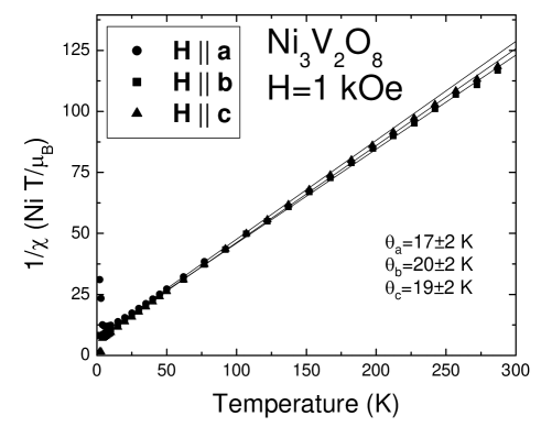
Figure 19: Determination of the Curie-Weiss temperatures $\Theta_{\alpha}$ from the high-temperature susceptibility data.Gavin

We next estimate the anisotropy $K$. Figure 18 implies that the LTI phase appears between the HTI and the C phases only when $K/J_{1}\sim 1/2$. This value is also roughly consistent with the anisotropy of the susceptibility.

Given these constraints, we propose a possible set of exchange parameters:

$$J_{1} = 10\ ,\ \ J_{2}=4\ ,\ \ J_{\rm av}=3\ ,$$

$$J_{b} = J_{c}=2\ ,\ \ {\rm and}\ \ K=5\ ,$$ (75)

all in units of K. The uncertainties are probably of order 50%. Substituting these values into Eq. (39) then yields the mean field transition temperature $T_{\rm PH}\approx 20$K, which is about 2.2 times the actual transition temperature. This reduction from the mean field estimate must result from fluctuations. In ideal Kagomé geometry one might think that $J_{\rm av}$ and $J_{1}$ would be identical. However, in NVO the Ni-O-Ni bond anglesRogado for $J_{1}$ ($95.0^{\rm o}$ and $90.4^{\rm o}$) are further from $90^{\rm o}$ than those for $J_{\rm av}$ ($90.3^{\rm o}$ and $91.5^{\rm o}$), which explains why $J_{1}$ is larger than $J_{\rm av}$. Our estimates for the DM and PD parameters were already given in Secs. V.1.2 and V.1.3.

VI Conclusions

In this paper we have presented a comprehensive investigation of the magnetic phase diagram of NVO. Here we summarize our conclusions and call attention to a number of topics for future research. Our conclusions are

1) The magnetic structures of the HTI, LTI and C magnetic phases of NVO have been closely determined. However, there are still some uncertainties in the structure: some of the complex phases of the various complex order parameters are not determined with precision. In addition, for the LTI phase neutron diffraction data, on its own, does not unambiguously identify whether the additional representation which is characteristic of the LTI phase is $\Gamma_{1}$ or $\Gamma_{2}$. However, the symmetry analysis of the spontaneous polarization (see Ref. FERRO, ) indicates that the correct choice is $\Gamma_{1}$.

2) We showed that a model having nearly isotropic interactions between nn and nnn on a spine and with single ion anisotropy can explain qualitatively the observed structures. (See Fig. 18.) In particular, the experimental determination of the incommensurate wavevector accurately determines the ratio $J_{1}/J_{2}$ of nearest- to next-nearest-neighbor interactions on a spine.

3) Using the experimental values for the P to HTI transition temperature and the Curie-Weiss temperatures (of the high temperature uniform susceptibility), we obtain the estimates $J_{1}\sim 10$K and $J_{2}\sim 4$K.

4) From the appearance of small off-axis components of the magnetization in the HTI phase we obtain estimates in the range $|D|\sim 0.5$K for the Dzyaloshinskii-Moriya interactions between adjacent Ni spine spins.

5) From the appearance of a weak FM moment in the commensurate AF phases (and the appearance of transverse spin components in the HTI phase) we conclude the existence of either anisotropic symmetric exchange interactions or, more probably, Dzyaloshinskii-Moriya antisymmetric spine-cross-tie exchange interactions. Both interactions are permitted by crystal symmetry and we give very crude estimates of their values.

6) We have provided a qualitative explanation for the shape of the phase boundaries between the various ordered and paramagnetic phases. In principle the shape of these phase boundaries can be used to deduce additional microscopic interactions. However, there are currently too many unknown parameters to allow this program to be carried out.

This work suggests several fruitful lines of future research, some of which are ongoing. Since the nn and nnn interactions along the spine are of the same order of magnitude, it would be interesting to alter the geometry of the coordinating oxygen ions. This might be done by applying pressure, or possibly uniaxial stress. Changing the ratio of these interactions would profoundly affect the magnetic properties of NVO. It is even possible that the magneto-electric properties could be grossly affected. Such experiments could greatly expand the emerging understanding of the magnetoelectric behavior of frustrated quantum magnets.

Appendix A Magnetic group theory analysis

Using the space group symmetry of the crystal structure we identify allowed basis vectors for a magnetic structure with the observed wave-vectors ${\bf v}$. This is done by determining the irreps and eigenvectors of the little group $G_{{\bf v}}$ of symmetry operations that leave the wave-vectors ${\bf v}$ invariant. The eigenvectors $\phi^{\lambda}$ of the $\lambda$-th irreps $\Gamma^{\lambda}$ were determined using the projector method.Heine They are given by

$$\phi^{\lambda}=\sum_{g}\chi^{\lambda}(g)g(\phi)\,,$$ (76)

where $g$ is an element of the little group and $\phi$ is any vector of the order parameter space. $\chi^{\lambda}(g)$ is character of symmetry element g in the representation $\Gamma^{\lambda}$.

The symmetry elements of the Cmca space group of NVO are given in Table 2. Note that this space group is nonsymmorphic because some of the group elements $\{{\cal O}|{\bf a}\}$ consist of a reflection or rotation ${\cal O}$ and require a translation ${\bf a}$ equal to half a direct lattice vector.

A.1 Commensurate structure

The ordering wave-vector ${\bf v}=(0,0,0)$ is invariant under all these operations so that the little group $G_{\bf v}$ contains all the elements of the space group. The group consists of $8$ different classes and therefore has $8$ irreps, all of which are one dimensional. We determined the classes and the character table of this group and these are shown in Table 4.

		$1$	$2_{b}$	$2_{a}$	$2_{c}$	$\overline{1}$	$m_{ac}$	$m_{bc}$	$m_{ab}$
	$\Gamma^{1}$	1	1	1	1	1	1	1	1
	$\Gamma^{2}$	1	1	1	1	-1	-1	-1	-1
	$\Gamma^{3}$	1	1	-1	-1	1	1	-1	-1
	$\Gamma^{4}$	1	1	-1	-1	-1	-1	1	1
	$\Gamma^{5}$	1	-1	1	-1	1	-1	1	-1
	$\Gamma^{6}$	1	-1	1	-1	-1	1	-1	1
	$\Gamma^{7}$	1	-1	-1	1	1	-1	-1	1
	$\Gamma^{8}$	1	-1	-1	1	-1	1	1	-1

Table 4: Irreducible representation of the group $G_{\bf v}$ for the commensurate magnetic structure with ${\bf v}=(0,0,0)$.

The eigenvectors were calculated using the projector method (See Eq. (76).) and are given in Table 5.

	$\psi_{1}$	$\psi_{2}$	$\psi_{3}$	$\psi_{4}$	$\psi_{5}$	$\psi_{6}$	$\psi_{7}$	$\psi_{8}$
${\bf m}_{s1}$	$\begin{array}[]{c}0\\ m^{b}_{s}\\ 0\end{array}$	$\begin{array}[]{c}0\\ m^{b}_{s}\\ 0\end{array}$	$\begin{array}[]{c}0\\ m^{b}_{s}\\ 0\end{array}$	$\begin{array}[]{c}0\\ m^{b}_{s}\\ 0\end{array}$	$\begin{array}[]{c}m^{a}_{s}\\ 0\\ m^{c}_{s}\end{array}$	$\begin{array}[]{c}m^{a}_{s}\\ 0\\ m^{c}_{s}\end{array}$	$\begin{array}[]{c}m^{a}_{s}\\ 0\\ m^{c}_{s}\end{array}$	$\begin{array}[]{c}m^{a}_{s}\\ 0\\ m^{c}_{s}\end{array}$
${\bf m}_{s2}$	$\begin{array}[]{c}0\\ -m^{b}_{s}\\ 0\end{array}$	$\begin{array}[]{c}0\\ -m^{b}_{s}\\ 0\end{array}$	$\begin{array}[]{c}0\\ m^{b}_{s}\\ 0\end{array}$	$\begin{array}[]{c}0\\ m^{b}_{s}\\ 0\end{array}$	$\begin{array}[]{c}m^{a}_{s}\\ 0\\ -m^{c}_{s}\end{array}$	$\begin{array}[]{c}m^{a}_{s}\\ 0\\ -m^{c}_{s}\end{array}$	$\begin{array}[]{c}-m^{a}_{s}\\ 0\\ m^{c}_{s}\end{array}$	$\begin{array}[]{c}-m^{a}_{s}\\ 0\\ m^{c}_{s}\end{array}$
${\bf m}_{s3}$	$\begin{array}[]{c}0\\ m^{b}_{s}\\ 0\end{array}$	$\begin{array}[]{c}0\\ -m^{b}_{s}\\ 0\end{array}$	$\begin{array}[]{c}0\\ m^{b}_{s}\\ 0\end{array}$	$\begin{array}[]{c}0\\ -m^{b}_{s}\\ 0\end{array}$	$\begin{array}[]{c}m^{a}_{s}\\ 0\\ m^{c}_{s}\end{array}$	$\begin{array}[]{c}-m^{a}_{s}\\ 0\\ -m^{c}_{s}\end{array}$	$\begin{array}[]{c}m^{a}_{s}\\ 0\\ m^{c}_{s}\end{array}$	$\begin{array}[]{c}-m^{a}_{s}\\ 0\\ -m^{c}_{s}\end{array}$
${\bf m}_{s4}$	$\begin{array}[]{c}0\\ -m^{b}_{s}\\ 0\end{array}$	$\begin{array}[]{c}0\\ m^{b}_{s}\\ 0\end{array}$	$\begin{array}[]{c}0\\ m^{b}_{s}\\ 0\end{array}$	$\begin{array}[]{c}0\\ -m^{b}_{s}\\ 0\end{array}$	$\begin{array}[]{c}m^{a}_{s}\\ 0\\ -m^{c}_{s}\end{array}$	$\begin{array}[]{c}-m^{a}_{s}\\ 0\\ m^{c}_{s}\end{array}$	$\begin{array}[]{c}-m^{a}_{s}\\ 0\\ m^{c}_{s}\end{array}$	$\begin{array}[]{c}m^{a}_{s}\\ 0\\ -m^{c}_{s}\end{array}$
${\bf m}_{c1}$	$\begin{array}[]{c}m^{a}_{c}\\ 0\\ 0\end{array}$		$\begin{array}[]{c}0\\ m^{b}_{c}\\ m^{c}_{c}\end{array}$		$\begin{array}[]{c}m^{a}_{c}\\ 0\\ 0\end{array}$		$\begin{array}[]{c}0\\ m^{b}_{c}\\ m^{c}_{c}\end{array}$
${\bf m}_{c2}$	$\begin{array}[]{c}-m^{a}_{c}\\ 0\\ 0\end{array}$		$\begin{array}[]{c}0\\ m^{b}_{c}\\ -m^{c}_{c}\end{array}$		$\begin{array}[]{c}m^{a}_{c}\\ 0\\ 0\end{array}$		$\begin{array}[]{c}0\\ -m^{b}_{c}\\ m^{c}_{c}\end{array}$

Table 5: Irreducible representations for the commensurate phase described with ${\bf v}=(0,0,0)$ for both the ${\rm Ni_{s}}$ and ${\rm Ni_{c}}$ sites. The components of the vector correspond to the spin component on the Ni sites in the order given in Table 3.

A.2 Incommensurate structure

For the ordering wave-vector ${\bf v}=(q,0,0)$, the little group $G_{\bf v}$ contains the following four elements of the space group:

$$\{1,\;2_{x},\;m_{xy},\;m_{xz}\}\,,$$ (77)

The group consists of $4$ different classes and therefore has $4$ one-dimensional irreps. We determined the classes and the character table of this group and these are shown in Table 6.

		$1$	$2_{a}$	$m_{ac}$	$m_{ab}$
	$\Gamma^{1}$	1	1	1	1
	$\Gamma^{2}$	1	1	$-1$	$-1$
	$\Gamma^{3}$	1	$-1$	$1$	$-1$
	$\Gamma^{4}$	1	$-1$	$-1$	$1$

Table 6: Irreducible representation of the group $G_{\bf v}$ for the incommensurate magnetic structure with ${\bf v}=(q,0,0)$.

The eigenvectors were calculated using the projector method using Eq.  (76) and are given in Table 7.

	$\psi_{1}$	$\psi_{2}$	$\psi_{3}$	$\psi_{4}$
${\bf m}_{s}^{1}$	$\begin{array}[]{c}m^{a}_{s}\\ m^{b}_{s}\\ m^{c}_{s}\end{array}$	$\begin{array}[]{c}m^{a}_{s}\\ m^{b}_{s}\\ m^{c}_{s}\end{array}$	$\begin{array}[]{c}m^{a}_{s}\\ m^{b}_{s}\\ m^{c}_{s}\end{array}$	$\begin{array}[]{c}m^{a}_{s}\\ m^{b}_{s}\\ m^{c}_{s}\end{array}$
${\bf m}_{s}^{2}$	$\begin{array}[]{c}m^{a}_{s}\\ -m^{b}_{s}\\ -m^{c}_{s}\end{array}$	$\begin{array}[]{c}m^{a}_{s}\\ -m^{b}_{s}\\ -m^{c}_{s}\end{array}$	$\begin{array}[]{c}-m^{a}_{s}\\ m^{b}_{s}\\ m^{c}_{s}\end{array}$	$\begin{array}[]{c}-m^{a}_{s}\\ m^{b}_{s}\\ m^{c}_{s}\end{array}$
${\bf m}_{s}^{3}$	$\begin{array}[]{c}-m^{a}_{s}\\ m^{b}_{s}\\ -m^{c}_{s}\end{array}$	$\begin{array}[]{c}m^{a}_{s}\\ -m^{b}_{s}\\ m^{c}_{s}\end{array}$	$\begin{array}[]{c}-m^{a}_{s}\\ m^{b}_{s}\\ -m^{c}_{s}\end{array}$	$\begin{array}[]{c}m^{a}_{s}\\ -m^{b}_{s}\\ m^{c}_{s}\end{array}$
${\bf m}_{s}^{4}$	$\begin{array}[]{c}-m^{a}_{s}\\ -m^{b}_{s}\\ m^{c}_{s}\end{array}$	$\begin{array}[]{c}m^{a}_{s}\\ m^{b}_{s}\\ -m^{c}_{s}\end{array}$	$\begin{array}[]{c}m^{a}_{s}\\ m^{b}_{s}\\ -m^{c}_{s}\end{array}$	$\begin{array}[]{c}-m^{a}_{s}\\ -m^{b}_{s}\\ m^{c}_{s}\end{array}$
${\bf m}_{c}^{1}$	$\begin{array}[]{c}m^{a}_{c}\\ 0\\ 0\end{array}$	$\begin{array}[]{c}m^{a}_{c}\\ 0\\ 0\end{array}$	$\begin{array}[]{c}0\\ m^{b}_{c}\\ m^{c}_{c}\end{array}$	$\begin{array}[]{c}0\\ m^{b}_{c}\\ m^{c}_{c}\end{array}$
${\bf m}_{c}^{2}$	$\begin{array}[]{c}-m^{a}_{c}\\ 0\\ 0\end{array}$	$\begin{array}[]{c}m^{a}_{c}\\ 0\\ 0\end{array}$	$\begin{array}[]{c}0\\ m^{b}_{c}\\ -m^{c}_{c}\end{array}$	$\begin{array}[]{c}0\\ -m^{b}_{c}\\ m^{c}_{c}\end{array}$

Table 7: Irreducible representations for the incommensurate phase associated with ${\bf v}=(q,0,0)$ for the ${\rm Ni_{s}}$ and ${\rm Ni_{c}}$ sites. The components of the vector correspond to the spin component on the Ni sites in the order given in Table 3.

As explained in the text, we replace the variables in the above table by symmetry adapted coordinates, so that we parametrize the eigenvectors as in Table 8.

To fit to data one assumes a single irrep and then optimizes with respect to the choice of the complex-valued amplitudes $m_{s}^{a}$, $m_{s}^{b}$, etc. For the HTI phase one selects the representation which best fits the data for the optimized values of the amplitudes. Alternatively, one can introduce the symmetry adapted coordinates as in Eqs. (8) and accept the conclusion from Landau theory that these symmetry adapted coordinates all have the same complex phase. These symmetry adapted coordinates are constructed by the methods leading to Eqs. (8) and are given in Table 8.

	$\psi_{1}$	$\psi_{2}$	$\psi_{3}$	$\psi_{4}$
${\bf m}_{s}^{1}$	$\begin{array}[]{c}i\tilde{m}_{sa}\\ \tilde{m}_{sb}\\ i\tilde{m}_{sc}\end{array}$	$\begin{array}[]{c}\tilde{m}_{sa}\\ i\tilde{m}_{sb}\\ \tilde{m}_{sc}\end{array}$	$\begin{array}[]{c}i\tilde{m}_{sa}\\ \tilde{m}_{sb}\\ i\tilde{m}_{sc}\end{array}$	$\begin{array}[]{c}\tilde{m}_{sa}\\ i\tilde{m}_{sb}\\ \tilde{m}_{sc}\end{array}$
${\bf m}_{s}^{2}$	$\begin{array}[]{c}i\tilde{m}_{sa}\\ -\tilde{m}_{sb}\\ -i\tilde{m}_{sc}\end{array}$	$\begin{array}[]{c}\tilde{m}_{sa}\\ -i\tilde{m}_{sb}\\ -\tilde{m}_{sc}\end{array}$	$\begin{array}[]{c}-i\tilde{m}_{sa}\\ \tilde{m}_{sb}\\ i\tilde{m}_{sc}\end{array}$	$\begin{array}[]{c}-\tilde{m}_{sa}\\ i\tilde{m}_{sb}\\ \tilde{m}_{sc}\end{array}$
${\bf m}_{s}^{3}$	$\begin{array}[]{c}-i\tilde{m}_{sa}\\ \tilde{m}_{sb}\\ -i\tilde{m}_{sc}\end{array}$	$\begin{array}[]{c}\tilde{m}_{sa}\\ -i\tilde{m}_{sb}\\ \tilde{m}_{sc}\end{array}$	$\begin{array}[]{c}-\tilde{m}_{sa}\\ i\tilde{m}_{sb}\\ -\tilde{m}_{sc}\end{array}$	$\begin{array}[]{c}\tilde{m}_{sa}\\ -i\tilde{m}_{sb}\\ \tilde{m}_{sc}\end{array}$
${\bf m}_{s}^{4}$	$\begin{array}[]{c}-i\tilde{m}_{sa}\\ -\tilde{m}_{sb}\\ i\tilde{m}_{sc}\end{array}$	$\begin{array}[]{c}\tilde{m}_{sa}\\ i\tilde{m}_{sb}\\ -\tilde{m}_{sc}\end{array}$	$\begin{array}[]{c}\tilde{m}_{sa}\\ i\tilde{m}_{sb}\\ -\tilde{m}_{sc}\end{array}$	$\begin{array}[]{c}-\tilde{m}_{sa}\\ -i\tilde{m}_{sb}\\ \tilde{m}_{sc}\end{array}$
${\bf m}_{c}^{1}$	$\begin{array}[]{c}\tilde{m}_{ca}\\ 0\\ 0\end{array}$	$\begin{array}[]{c}\tilde{m}_{ca}\\ 0\\ 0\end{array}$	$\begin{array}[]{c}0\\ \tilde{m}_{cb}\\ \tilde{m}_{cc}\end{array}$	$\begin{array}[]{c}0\\ \tilde{m}_{cb}\\ \tilde{m}_{cc}\end{array}$
${\bf m}_{c}^{2}$	$\begin{array}[]{c}-\tilde{m}_{ca}\\ 0\\ 0\end{array}$	$\begin{array}[]{c}\tilde{m}_{ca}\\ 0\\ 0\end{array}$	$\begin{array}[]{c}0\\ \tilde{m}_{cb}\\ -\tilde{m}_{cc}\end{array}$	$\begin{array}[]{c}0\\ -\tilde{m}_{cb}\\ \tilde{m}_{cc}\end{array}$

Table 8: Symmetry adapted coordinates which transform according to the irreps for the incommensurate phase associated with ${\bf v}=(q,0,0)$ for the Ni_s and Ni_c sites. When more than one representation is active, it is a reasonable approximation to allow all parameters of representation $\Gamma_{n}$ to have the same phase factor $e^{i\phi_{n}}$.

Appendix B Magnetic neutron scattering cross-section

The integrated intensity of magnetic Bragg peaks is related to the structure factor of the magnetic ordering through Lovesey_book

$$I({\bf Q})=\left(\frac{\gamma r_{0}}{2}\right)^{2}N_{m}\frac{(2\pi)^{3}}{V_{m0}}\Phi\;R({\bf Q})\;|f({\bf Q})|^{2}|{\bf F}_{\bot}({\bf Q})|^{2}\,,$$ (78)

where $f({\bf Q})$ is the magnetic form factor for Ni²⁺ ions.IntTables $\Phi$ is the flux of incident neutrons, $N_{m}$ and $V_{m0}$ are the number and the volume of the magnetic unit cells, $\gamma=-1.913$ and $r_{0}=2.818\cdot 10^{-15}\;\mathrm{m}$. $I({\bf Q})$ is the total integrated intensity of a Bragg reflection when the sample is rotated about the normal to the scattering plane and $R({\bf Q})$ is a factor which takes into account the ${\bf Q}$-dependent sensitivity of the spectrometer. For the powder experiment, $R({\bf Q})$=$1/\sin(\theta(\bf Q))$. For the triple-axis experiment, $R({\bf Q})$ was calculated using the Cooper-Nathans approximation.Cooper_Nathans ${\bf F}_{\bot}({\bf Q})$ is the component of the magnetic structure factor perpendicular to the scattering wave vector and is defined as

$${\bf F}_{\bot}({\bf Q})={\bf F}({\bf Q})-({\bf F}({\bf Q})\cdot{\bf\hat{Q}})\;{\bf\hat{Q}},$$ (79)

where ${\bf\hat{Q}}={\bf Q}/Q$.

The magnetic structure factor for a commensurate structure was calculated using

$${\bf F}({\bf Q})=\sum_{i}{\bf m}_{i}\exp(-{\rm i}\;{\bf Q}\cdot{\bf d}_{i})$$ (80)

where ${\bf d}_{i}$ are the positions of the Ni²⁺-ions and the sum is over the magnetic ions in the magnetic unit cell. The magnetic dipole moments ${\bf m}_{i}$ are given by one of the irreps given in Table 5. For incommensurate structures the magnetic structure factor was calculated using

$${\bf F}({\bf Q})=\sum_{i}\frac{1}{2}\;{\bf\Psi}^{\bf v}_{i}\exp(-{\rm i}\;{\bf Q}\cdot{\bf d}_{i})\,,$$ (81)

where the Fourier components of the structure, $\Psi^{\bf v}_{i}$, are given by the basis vectors of the irreps of the little group given in Table 7. The moment on site $i$ is given by ${\bf m}_{i}$=$\frac{1}{2}({\bf\Psi}^{\bf v}+({\bf\Psi}^{\bf v})^{\star})$, so the factor $\frac{1}{2}$ in Eq.  (81) ensures that the scale factor for the basis vectors of the irreps can be expressed in Bohr magnetons.

Appendix C Absolute magnitude of the ordered moment

The magnitude of the ordered moments were determined by comparing the nuclear and the AF Bragg peak intensities. The intensity of a nuclear Bragg peak is given as

$$I({\bf Q})=N_{uc}\frac{(2\pi)^{3}}{V_{0}}\Phi\;R({\bf Q})\;|F_{N}({\bf Q})|^{2}\,,$$ (82)

where $N_{uc}$ and $V_{0}$ are the number and the volume of the unit cells. $F_{N}({\bf Q})$ is the nuclear structure factor given asSquires

$$F_{N}({\bf Q})=\sum_{i}b_{i}\exp(-{\rm i}\,{\bf Q}\cdot{\bf d}_{i})\,,$$ (83)

where the sum runs over all elements in the nuclear unit cell and $b_{i}$ is the bound coherent scattering lengthIntTables of atom $i$ in the unit cell. Since multiple scattering and extinction corrections were important for the strongest reflections of the single crystal, their intensities were ignored for the normalization. The measured nuclear intensities gave the overall scale factor $A_{\rm exp}=N_{uc}\frac{(2\pi)^{3}}{V_{0}}\Phi$ in Eq  (82). The magnitude of the ordered magnetic moment was determined using $A_{\rm exp}$ and Eq.  (78), allowing then the determination of the ordered moment for the various structures.

References

- (1) S. Sachdev, Phys. Rev. B 45, 12377 (1992).
- (2) P. Sindzingre, G. Misguic, C. Lhuillier, B. Bernu, L. Pierre, Ch. Waldtmann, and H.-U. Everts, Phys. Rev. Lett. 84, 2953 (2000).
- (3) S.-H. Lee, C. Broholm, G. Aeppli, T. G. Perring, and B. Hessen, Phys. Rev. Lett. 76, 4424 (1996).
- (4) C. Broholm, G. Aeppli, G. P. Espinosa, and A. S. Cooper, Phys. Rev. Lett. 65, 3173 (1990).
- (5) S.-H. Lee, C. Broholm, G. Aeppli, A. P. Ramirez, T. G. Perring, C. Carlisle, M. Adams, and B. Hessen, Europhys. Lett. 35, 127 (1996).
- (6) S.-H. Lee, C. Broholm, M. F. Collins, L. Heller, A. P. Ramirez, Ch. Kloc, E. Bucheri, R. W. Erwin, and N. Lacevic, Phys. Rev. B 56, 8091 (1997).
- (7) D. Grohol, Q. Huang, B. H. Toby, J. W. Lynn, Y. S. Lee, and D. G. Nocera, Phys. Rev. B 68, 094404 (2003).
- (8) G. Lawes, A. B. Harris, T. Kimura, N. Rogado, R. J. Cava, A. Aharony, O. Entin-Wohlman, T. Yildirim, M. Kenzelmann, C. Broholm, and A. P. Ramirez, Phys. Rev. Lett. 95, 087205 (2005).
- (9) A. B. Harris, T. Yildirim, A. Aharony, and O. Entin-Wohlman, to be published.
- (10) N. Rogado, G. Lawes, D. A. Huse, A. P. Ramirez, and R. J. Cava, Solid State Comm. 124, 229 (2002).
- (11) G. Lawes, M. Kenzelmann, N. Rogado, K. H. Kim, G. A. Jorge, R. J. Cava, A. Aharony, O. Entin-Wohlman, A. B. Harris, T. Yildirim, Q. A. Huang, S. Park, C. Broholm, and A. P. Ramirez, Phys. Rev. Lett. 93, 247201 (2004).
- (12) A. B. Harris et al., unpublished.
- (13) E. E. Sauerbrei, F. Faggiani, and C. Calvo, Acta Crystallogr. B 29, 2304 (1973).
- (14) A. Larson and R. V. Dreele, Los Alamos National Laboratory Report No. LAUR086-748, 1990.
- (15) A. J. C. Wilson, International Tables For Crystallography (Kluwer Academic Publishers, Dordrecht, 1995), Vol. A.
- (16) F. C. Chou, A. Aharony, R. J. Birgeneau, O. Entin-Wohlman, M. Greven, A. B. Harris, M. A. Kastner, Y. J. Kim, D. S. Kleinberg, Y. S. Lee, and Q. Zhu, Phys. Rev. Lett. 78, 535 (1997).
- (17) V. Kiryukhin, Y. J. Kim, K. J. Thomas, F. C. Chou, R. W. Erwin, Q. Huang, M. A. Kastner, and R. J. Birgeneau, Phys. Rev. B 63, 144418 (2001).
- (18) S. Tornow, O. Entin-Wohlman, and A. Aharony, Phys. Rev. B 60, 10206 (1999).
- (19) Our convention for wavevectors (in r. l. u.) is that the -component is measured in units of , the -component in units of and the component in units of . Lower case Roman letters (except ) denote integer components, whereas and denote general noninteger values. In expressions such as , and must be taken in compatible units
- (20) V. Heine, in Group Theory in Quantum Mechanics (Dover Publications, New York, 1993), pp. 119, 288.
- (21) I. E. Dzyaloshinskii, Sov. Phys. JETP 5, 1259 (1957).
- (22) L. D. Landau and E. M. Lifshitz, Statistical Physics (Pergamon, London, 1958).
- (23) J. Schweizer, C. R. Physique 6, 375 (2005)
- (24) T. Nagamiya, in Solid State Physics, edited by F. Seitz and D. Turnbull (Academic, New York, 1967), Vol. 29, p. 346.
- (25) T. A. Kaplan, Phys. Rev. 124, 329 (1961).
- (26) S. Aubry, in Solitons and Condensed Matter Physics, edited by A. Bishop and T. Schneider (Springer Verlag, Berlin, 1978), p. 264.
- (27) M. E. Fisher and W. Selke, Phys. Rev. Lett. 44, 1502 (1980).
- (28) I. Dzyaloshinskii, J. Phys. Chem. Solids 4, 241 (1958).
- (29) T. Moriya, Phys. Rev. 120, 91 (1960).
- (30) A. D. Bruce and A. Aharony, Phys. Rev. B 11, 478 (1975).
- (31) T. Yildirim, A. B. Harris, O. Entin-Wohlman, and A. Aharony, Phys. Rev. Lett. 72, 3710 (1994).
- (32) R. Sachidanandam, T. Yildirim, A. B. Harris, A. Aharony, and O. Entin-Wohlman, Phys. Rev. B 56, 260 (1997).
- (33) M. A. Kastner, A. Aharony, R. J. Birgeneau, F. C. Chou, O. Entin-Wohlman, M. Greven, A. B. Harris, Y. J. Kim, Y. S. Lee, M. E. Parks, and Q. Zhu, Phys. Rev. B 59, 14702 (1999).
- (34) K. D. Bowers and J. Owen, Rep. Prg. Phys. 18, 304 (1955).
- (35) G. Lawes, unpublished.
- (36) S. W. Lovesey, Theory of Neutron Scattering from Condensed Matter (Clarendon Press, Oxford, 1984).
- (37) A. J. C. Wilson, International Tables For Crystallography (Kluwer Academic Publishers, Dordrecht, 1995), Vol. C.
- (38) M. J. Cooper and R. Nathans, Acta Crys. 23, 357 (1967).
- (39) G. L. Squires, Thermal Neutron Scattering (Cambridge University Press, Cambridge, 1978).