Ferromagnetic Properties of ZrZn₂

Abstract

The low Curie temperature ($T_{C}\approx 28$ K) and small ordered moment ($M_{0}\approx 0.17$ $\mu_{\mathrm{B}}$f.u.^-1) of ZrZn₂ make it one of the few examples of a weak itinerant ferromagnet. We report results of susceptibility, magnetization, resistivity and specific heat measurements made on high-quality single crystals of ZrZn₂. From magnetization scaling in the vicinity of $T_{C}$ ($0.001<|T-T_{C}|/T_{C}<0.08$), we obtain the critical exponents $\beta=0.52\pm 0.05$ and $\delta=3.20\pm 0.08$, and $T_{C}=27.50\pm 0.05$ K. Low-temperature magnetization measurements show that the easy axis is [111]. Resistivity measurements reveal an anomaly at $T_{C}$ and a non-Fermi liquid temperature dependence $\rho(T)=\rho_{0}+AT^{n}$, where $n=1.67\pm 0.02$, for $1<T<14$ K. The specific heat measurements show a mean-field-like anomaly at $T_{C}$. We compare our results to various theoretical models.

PACS, the Physics and Astronomy

I Introduction

Ferromagnetism in the cubic Laves compound ZrZn₂ was discovered by Matthias and Bozorth Matthias and Bozorth (1958) in 1958. Its occurrence in ZrZn₂ is unusual because neither elemental Zr nor Zn is magnetically ordered. The low Curie temperature and small ordered moment of ZrZn₂ make it one of the few examples of a small-moment or weak itinerant ferromagnet. ZrZn₂ was initially considered to be a candidate for Stoner theory Stoner (1936). However a quantitative comparison of Stoner theory with experiment suggests that spin fluctuation effects are important Moriya (1985). In particular, the Curie temperature is strongly renormalized downwards from the Stoner value estimated from band structure parameters Kübler (2004).

ZrZn₂ crystallizes in the C15 cubic Laves structure shown in Fig.1, with lattice constant $a=7.393$ Å. The Zr atoms form a tetrahedrally coordinated diamond structure and the magnetic properties of the compound derive from the Zr 4d orbitals, which have a significant direct overlap leading to the magnetic moment being spread out over the network shown by the thick lines in Fig. 1. ZrZn₂ is strongly unsaturated: an applied field of 5.7 T results in a 50 % increase in the ordered moment. In contrast, strong ferromagnets such as Fe and Ni show a negligible increase of the ordered moment with field after a single domain is formed. The unsaturated behavior of ZrZn₂ indicates a large longitudinal susceptibility and the presence of longitudinal spin fluctuations Murata and Doniach (1972); Lonzarich and Taillefer (1985). Further evidence for the existence of strong spin fluctuations in ZrZn₂ is provided by the remarkably large effective mass of its quasiparticles Yates et al. (2003). The low-temperature specific heat coefficient Pfleiderer et al. (2001a) and the calculated DOS at the Fermi Level Yates et al. (2003) imply an average mass enhancement $1+\lambda\approx 5$ at zero applied magnetic field dHv . This is the largest known average mass enhancement for a $d$-band metal, and is even slightly larger than that of the strongly-correlated oxide system Sr₂RuO₄ for which $1+\lambda\approx 3.6$ [Refs. Mackenzie et al., 1996; Bergemann et al., 2003].

It has been known for some time that the ferromagnetism of ZrZn₂ is extremely sensitive to pressure Smith et al. (1971). Recent experiments on the samples studied here Uhlarz et al. (2004a) have shown that a pressure of $p_{c}=16.5$ kbar causes the ferromagnetism to disappear with a first order transition. Thus we may also view ZrZn₂ as being close to a quantum critical point (QCP) Uhlarz et al. (2004a); Kimura et al. (2004). In view of the strong longitudinal fluctuations present in ZrZn₂ and its proximity to a QCP, it has been proposed as a candidate for magnetically mediated superconductivity Leggett (1978); Enz and Matthias (1978); Fay and Appel (1979); Pfleiderer et al. (2001b). However, as discussed elsewhere Yelland et al. , we find no evidence for bulk superconductivity at ambient pressure in these samples.

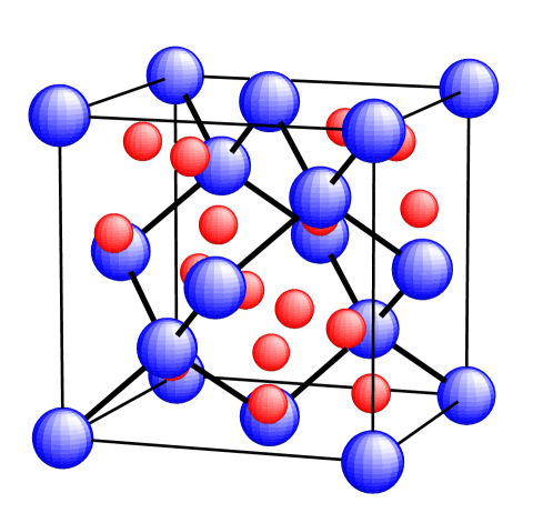
Figure 1: (Color online) The C15 structure of ZrZn₂. Zr atoms occupy the sites of the larger spheres.

There are surprisingly few measurements of the fundamental properties of high-quality samples (RRR$\geq$100) of ZrZn₂ in the literature. In this paper, we present a study of the transport and thermodynamic properties of ZrZn₂. In particular, we have measured the magnetocrystalline anisotropy, the magnetization isotherms for $2<T<40$ K and $0<B<5$ T; the resistivity from low temperatures through the Curie temperature; and the specific heat capacity for $0.3<T<40$ K. These properties contain information about the quasiparticles and magnetic interactions in ZrZn₂. For example, the temperature dependence of the resistivity at low temperatures gives information about the fundamental excitations that scatter quasiparticles, and the comparison of specific heat and magnetization data gives information about the importance of spin fluctuations in ZrZn₂.

II Experimental Details

II.1 Crystal Growth and Sample Quality

ZrZn₂ melts congruently at 1180^∘C [Refs. Elliott, 1965; Massalski et al., 1986]. At this temperature zinc has a vapor pressure of about 10 bars and is an aggressive flux. Thus we chose to grow ZrZn₂ by a directional cooling technique Schreurs et al. (1989). Stoichiometric quantities of high-purity zone-refined Zr (99.99%, Materials Research MARZ grade) and Zn (99.9999%, Metal Crystals) were loaded into a Y₂O₃ crucible. The total charge used was 4.2 g. The crucible was sealed inside a tantalum bomb which was closed by electron beam welding under vacuum. The assembly was heated to 1210^∘C and then cooled through the melting point at 2^∘C hr^-1. The ingot was then annealed by cooling to 500^∘C over a period of 72 hr. This method produced, on occasions, single crystals of volumes up to approximately 0.4 cm³. Single crystals produced in this way had residual resistivities as low as $\rho_{0}$= 0.53 $\mu\Omega\mathrm{cm}$ corresponding to a residual resistance ratio RRR = $\rho(293\,\mathrm{K})/\rho(T\rightarrow 0)$=105. With the exception of Ref. van Deursen et al., 1986, previous reports by other groups of the fundamental transport and thermodynamic properties of ZrZn₂ have been carried out on samples with RRR $\lesssim$ 45.

The residual resistivity $\rho_{0}$ and the Dingle temperature determined from de Haas-van Alphen measurements may be used to estimate the quasiparticle mean free path $\ell$ due to impurity scattering. For a crystal with cubic symmetry Ziman (1964),

$$\sigma=\frac{1}{4\pi^{3}}\frac{e^{2}\tau}{\hbar}\frac{1}{3}\int v_{F}\;dS_{F}=\frac{1}{4\pi^{3}}\frac{e^{2}}{\hbar}\frac{1}{3}\int\ell\;dS_{F}.$$ (1)

From band structure calculations Yates et al. (2003), we estimate the sum of the Fermi surface areas to be $S_{F}=$ $1.9\times 10^{21}\mathrm{m}^{-2}$. Hence $\ell_{\mathrm{trans}}=1350$ Å. A second estimate of the quasiparticle mean free path can be made from the de Haas-van Alphen effect Yates et al. (2003); values are in the range $\ell_{\mathrm{dHvA}}=$ 1500–2800 Å depending on Fermi surface orbit, in approximate agreement with $\ell_{\mathrm{trans}}$. In general, one expects that $\tau_{\mathrm{dHvA}}<\tau_{\mathrm{trans}}$ since $\tau_{\mathrm{trans}}$ is weighted towards large momentum changes Abrikosov et al. (1963), whereas $\tau_{\mathrm{dHvA}}$ weights all scattering equally. However, the opposite situation $\tau_{\mathrm{dHvA}}>\tau_{\mathrm{trans}}$ may also arise in an inhomogeneous sample, since the exponential scattering rate dependence of the Dingle factor $R_{D}=\exp(-\pi m_{b}/eB\tau)$ causes $\ell_{\mathrm{dHvA}}$ to be strongly weighted towards high quality regions of the sample. Given these considerations, the two mean free path estimates $\ell_{\mathrm{dHvA}}$ and $\ell_{\mathrm{trans}}$ are as consistent as can be expected.

II.2 Transport and Thermodynamic Measurements

Resistivity measurements were made using a standard a.c. technique using a Brookdeal 9433 low-noise transformer and SR850 digital lock-in amplifier with a measuring frequency $f$=2 Hz. Sample contacts were made with Dupont 4929 conducting Ag/epoxy. Measurements of a.c. susceptibility were made by a standard technique in which the sample was mounted inside a small coil of approximately 2500 turns. The system was calibrated using the superconducting transition of an indium sample of similar size to the ZrZn₂ sample. Magnetization measurements were made using a commercial Quantum Design MPMS-XL SQUID magnetometer.

Heat capacity measurements were made both by a long-pulse method and an a.c. method Carrington et al. (1997). In the long-pulse technique Shepherd (1985) the sample was mounted on a silicon platform connected to a temperature-controlled stage by a thin copper wire. In the a.c. technique the sample was mounted on a flattened 12 $\mu$m chromel-constantan thermocouple and heated optically. The long pulse technique allows an accurate determination of the absolute value of $C(T)$ but has relatively low resolution. The a.c. technique has much higher resolution ($\sim 0.1$%), and is thus ideally suited to resolving the small anomaly at $T_{C}$. However, it does not allow an accurate determination of the absolute value of $C(T)$ due to the poorly defined addenda contribution. We estimated the addenda by measuring a Cu sample with similar $C(T)$; the a.c. data with the estimated addenda subtracted were multiplied by a scale factor to match the long-pulse data at a single temperature.

III Results

III.1 Magnetization Isotherms and Scaling near the Ferromagnetic Transition

III.1.1 Low Temperature Isotherms

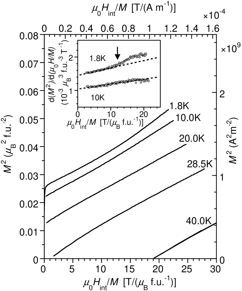
Figure 2: Arrott plot of magnetization isotherms in the temperature range $1.8\leq T\leq 40$ K. In the Stoner theory of a weak itinerant ferromagnet, $M^{2}$ is a linear function of $H/M$. Inset: the derivative $\mathrm{d}(M^{2})/\mathrm{d}(\mu_{0}H/M)$ of the 1.8 K and 10 K Arrott curves; the 1.8 K curve is offset by +5$\times 10^{-3}\,\mu_{\mathrm{B}}^{3}\,\mathrm{f.u.}^{-3}\,\mathrm{T}^{-1}$. Dotted lines are guides to the eye. Note the feature in the 1.8 K curve, indicated by an arrow.

Since the discovery of ZrZn₂ there have been many studies of the magnetic properties. Previous work Matthias and Bozorth (1958); Ogawa and Sakamoto (1967); Knapp et al. (1971); Smith et al. (1971); Ogawa (1976); Mattocks and Melville (1978); van Deursen et al. (1986); Grosche et al. (1995); Seeger et al. (1995); Pfleiderer et al. (2001b); Uhlarz et al. (2004b) has shown that the Curie temperature and the ordered moment, are strongly dependent on sample quality and composition Knapp et al. (1971). Thus the purpose of the present magnetization measurements is to attempt to characterize the magnetic properties in the clean limit. The high-quality of our samples is indicated by their low residual resistivity (RRR=105) and long mean free path, which has allowed much of the Fermi surface to be observed by the dHvA effect Yates et al. (2003).

Although many plots of the magnetization isotherms for ZrZn₂ have been reported Ogawa and Sakamoto (1967); Knapp et al. (1971); Mattocks and Melville (1978); van Deursen et al. (1986) improved instrumentation and higher sample quality have recently allowed fine structure to be observed. For a weak ferromagnet, the magnetization isotherms are generally expected to obey the Stoner form in which $M^{2}$ is a linear function of $H/M$. Fig. 2 is an Arrott plot of our magnetization isotherms. The near linearity of the isotherms confirms that they are indeed of approximately the expected form. However, the isotherm at $T=1.8$ K shows an intriguing feature at $\mu_{0}H\approx 2.4$ T, indicated by an arrow in Fig. 2. Another more pronounced feature is directly visible in the $T=1.75$ K $M(H)$ isotherm plotted in Ref. Pfleiderer et al., 2001b, at a field $\approx 6$ T, outside the range of our present measurements. Structure in the electronic DOS close to the Fermi level is expected to have a profound influence on $M(T,B)$ in itinerant ferromagnets Shimizu (1964, 1965), and calculations Yates et al. (2003) suggest that just such structure is present in the DOS of ZrZn₂, the Fermi level lying between two sharp peaks in the majority spin DOS. This is an interesting connection that could be explored in future work.

III.1.2 Scaling near $T_{C}$

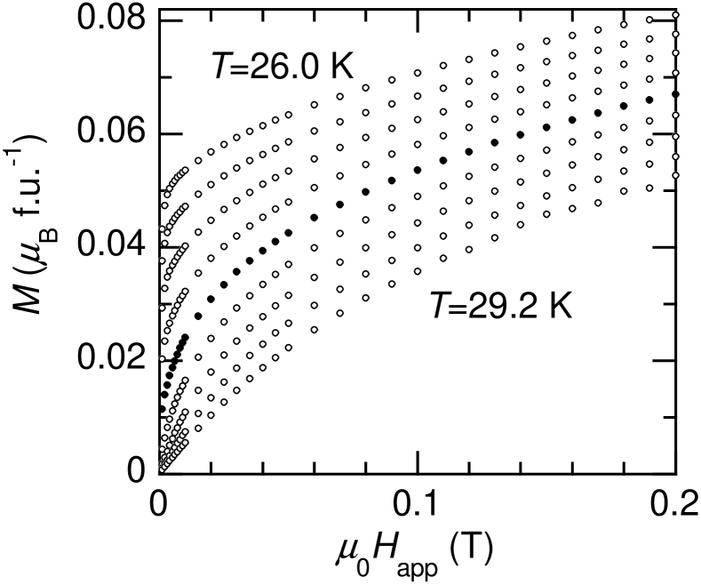
Figure 3: Low field magnetization isotherms near the ferromagnetic critical temperature of ZrZn₂ (near-critical isotherm at $T=27.6$ K shown by filled circles).

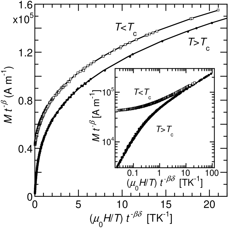
Figure 4: Scaling plot of magnetization isotherms of ZrZn₂ near $T_{C}$. The data shown here are the same as those in Fig. 3 except that we have excluded the region $\mu_{0}H<0.005$ T to avoid systematic errors due to multiple ferromagnetic domains inside the sample (see text). The correct choice of $T_{C}$, $\beta$ and $\delta$ causes the scaled data to collapse onto a single curve for $T<T_{C}$ and another for $T>T_{C}$. The values that allow the best fit to the scaled data of a 7^th order polynomial in $M^{*}$ are shown in Table 1. The solid lines show the best fit polynomials for $T<T_{C}$ and $T>T_{C}$. The inset shows the same data on log-log axes.

At temperatures approaching the Curie temperature of a ferromagnet the magnetization isotherms $M(H)$ become highly nonlinear making the identification of $T_{C}$ difficult. An accurate determination of $T_{C}$ can be achieved by a scaling analysis of the magnetization close to the transition; we have therefore measured magnetization isotherms at a set of temperatures near $T_{C}$ allowing us to determine $T_{C}$ and the magnetization scaling exponents.

Close to the critical temperature of a ferromagnetic transition, the magnetization $M(H,T)$ can be expressed as $M^{*}(h^{*})$ where $M^{*}=Mt^{-\beta}$ and $h^{*}=(H/T)t^{-\beta\delta}$ are appropriately scaled quantities Yeomans (1992). Here $t=|1-T/T_{C}|$ is the reduced temperature and $\beta$, $\delta$ are the critical exponents. The experimental determination of $\beta$ and $\delta$ allows remarkably universal conclusions to be drawn about the physical model which underlies the phase transition. We have measured the magnetization $M(H)$ in applied fields $0<\mu_{0}H<0.2$ T at closely spaced temperatures in the range $0.1\leq|T-T_{C}|<2.2$ K. Fig. 3 shows the raw data. In order to determine $T_{C}$ and the scaling exponents, $M^{*}$ and $h^{*}$ were calculated from the experimental data set for all values of $\beta,\delta$ and $T_{C}$ within a certain volume of the 3D parameter space encompassing both the Heisenberg and mean field models. For each combination of values, the polynomial in $M^{*}$ which best fit the scaled experimental values of $h^{*}$ was found, and its goodness-of-fit ($\chi^{2}$) value calculated. The correct parameter values are taken as those for which the best fit polynomial has the lowest $\chi^{2}$. Only data points for which $\mu_{0}H_{\mathrm{app}}\geq 0.005$ T are included in the scaling analysis in order to ensure the formation of a single ferromagnetic domain inside the sample. The data have been corrected for the small demagnetizing factor of this sample, $D=0.060$, but we note that the final results are barely affected by this. We find $T_{C}=(27.50\pm 0.05)$ K, $\beta=0.52\pm 0.05$ and $\delta=3.20\pm 0.08$ (see Table 1). The values of $\beta$ and $\delta$ are close to those obtained on lower quality samples with smaller $T_{C}$’s Seeger et al. (1995).

In order to interpret our scaling results, we need to know whether we are in the critical region. The Ginzburg criterion Chaikin and Lubensky (1995),

$$\Delta T_{\mathrm{G}}=\frac{T_{C}k_{\mathrm{B}}^{2}}{32\pi^{2}(\Delta C_{\mathrm{V}})^{2}\xi_{0}^{6}}$$ (2)

allows us to estimate the extent of the critical region. From neutron scattering measurements Bernhoeft et al. (1988) of the wavevector-dependent magnetic susceptibility $\chi(q)$ and low temperature magnetization measurements we estimate the magnetic correlation length $\xi_{0}=33$ Å. The specific heat jump is $\Delta C\approx 155$ mJ K^-1 mol^-1 (see section III.4). Hence $\Delta T_{\mathrm{G}}=0.4$ mK. Thus our data are collected outside the critical region where mean field behavior is expected. Table 1 shows that our results are indeed in agreement with the expected mean field results for a 3D ferromagnet. Finally, is it worth commenting that determining the Curie temperature $T_{c}$ from critical scaling, as described here, yields a lower value than that obtained by taking the peak in $(dM/dB)$ with $T$. This may explain the slightly higher values reported elsewhere Pfleiderer et al. (2001b) for similar samples.

Figure 5: Arrott plot of magnetization isotherms near $T_{C}$ for ZrZn₂. The isotherms were measured at 0.4 K intervals and at 0.1 K intervals close to $T_{C}$; the bold line is the critical isotherm at $T=27.5$ K. In the Stoner theory of a weak itinerant ferromagnet, $M^{2}$ is a linear function of $H/M$

Table 1: Theoretical critical exponents for various models of phase transition and the experimental values found in this work. $T_{C}$ was found to be 27.50$\pm$0.05 K.

	mean-field	Heisenberg	this work
$\beta$	0.5	0.326	0.52 $\pm$ 0.05
$\delta$	3	4.78	3.20 $\pm$ 0.08

Figure 6: The temperature dependence of the magnetization (filled circles) and the inverse susceptibility (open squares) as determined from Arrott plots.

III.2 Magnetocrystalline Anisotropy

Figure 7: Magnetic hysteresis curve for ZrZn₂ measured at $T=5$ K. The inset shows the central region magnified. Note the small coercive field $H_{\mathrm{coer}}\approx 0.05$ mT.

The exchange interaction in an itinerant electron system is often modelled as isotropic, depending only on the relative orientation of electron spins. However, the crystal field also enters the free energy via spin-orbit coupling, causing anisotropy of magnetic properties. One motivation for studying the magnetocrystalline anisotropy is that it has implications for the symmetry of the superconducting order parameter in the spontaneous mixed state of the putative superconducting phase of ZrZn₂ [Ref. Walker and Samokhin, 2002].

Fig. 7 shows a low-field hysteresis loop measured for applied fields in the range $-0.05$ T$<\mu_{0}H_{\mathrm{app}}<0.05$ T. The main panel shows that a field of approximately 5 mT is sufficient to create a single ferromagnetic domain. The inset reveals the low coercive field of the present samples $H_{\mathrm{coer}}\approx 0.05$ mT and justifies our method (see below) for obtaining the magnetic anisotropy constants.

We have determined the ferromagnetic anisotropy of ZrZn₂ from $M(H)$ isotherms at $T=5$ K. A disc-shaped sample (diameter $2R=2.72$ mm, thickness $t=0.47$ mm) was spark-cut so that the plane of the disc was (110). This geometry allows access to the three major cubic symmetry directions [100], [110] and [111] with the magnetic field in the plane of the disc so that the demagnetizing field is the same in each orientation. For this sample, the volume averaged demagnetizing factor is $D\approx 0.146$ [Ref. Crabtree, 1977], which for $M=0.16\,\mu_{\mathrm{B}}\,\mathrm{f.u.}^{-1}$ corresponds to an average demagnetizing field $\mu_{0}H_{\mathrm{D}}\approx 0.037$ T inside the sample. In this section we denote the measured magnetization by $M_{\parallel}$ to emphasize that the SQUID measurement is only sensitive to the component of $\mathbf{M}$ parallel to $\mathbf{H}_{\mathrm{app}}$, which is vital for extracting the anisotropy constants by the thermodynamic method described later. Fig. 8 shows $M_{\parallel}(H_{\mathrm{int}})$ measured with $H_{\mathrm{app}}$ parallel to each of the three symmetry directions; $H_{\mathrm{int}}$ is the internal field that, in a simple scalar notation, is approximately related to the applied field $H_{\mathrm{app}}$ by $H_{\mathrm{int}}=H_{\mathrm{app}}-DM$. As $H_{\mathrm{int}}$ increases from zero, a single domain is rapidly formed. The slower increase in $M_{\parallel}(H_{\mathrm{int}})$ for $\mu_{0}H_{\mathrm{int}}>0.003$ T with $\mathbf{H}_{\mathrm{app}}\parallel[001]$ or $[110]$, arises from the rotation of $\mathbf{M}$ away from the easy axis towards $\mathbf{H}_{\mathrm{int}}$ as the ratio of the interaction term $\mathbf{M}\cdot\mathbf{H}_{\mathrm{int}}$ to the anisotropy energy increases. Fig. 8 shows that saturation is reached most rapidly with $\mathbf{H}_{\mathrm{app}}\parallel[111]$, demonstrating that [111] is the ferromagnetic easy axis at this temperature.

Figure 8: Magnetization curves of a ZrZn₂ single crystal measured at $T=5$ K with field applied along [100] (dotted line), [110] (solid line) and [111] (dashed line). The ferromagnetic easy axis is seen to be [111] at this temperature. Upper inset: plot of Eq.(2) using values of $K_{1}$ and $K_{2}$ determined from $M_{\parallel}(H_{\mathrm{int}})$ as described in the text. Lower inset: $M_{\parallel}(H_{\mathrm{int}})$ up to 5 T for the same sample.

The principal cause of the rounding of the $M_{\parallel}(H_{\mathrm{int}})$ curve, even for $H\,\parallel[111]$, is likely to be the inhomogeneity of the demagnetizing field. The only practical sample shapes that give a uniform demagnetizing field are ellipsoids of revolution. We have calculated the volume distribution of the demagnetizing field for a perfect cylinder of the required aspect ratio assuming that the magnetization is uniform; the characteristic width of the distribution is $\delta D\sim 0.07$ and, for example, $\sim 12\%$ of the sample volume has a local demagnetizing field that exceeds the volume average value by a factor $>1.5$. Angular misalignments of up to $2^{\circ}$ may also contribute.

The first two terms in the standard expansion of the anisotropic free energy of a ferromagnet with cubic symmetry Williams (1937) can be expressed, for the present geometry, as

$$F(\theta)=\sin^{2}\theta(\cos^{2}\theta+\frac{1}{4}\sin^{2}\theta)K_{1}+\frac{1}{4}(\sin^{4}\theta\cos^{2}\theta)K_{2}$$ (3)

where $\theta$ is the angle within the (110) plane between $\mathbf{M}$ and [100] and $K_{1,2}$ are the first and second anisotropy constants. It is possible, in principle, to determine the anisotropy constants by assuming that $|\mathbf{M}|$ is fixed in the ‘approach to saturation’ region of the $M_{\parallel}(H_{\mathrm{int}})$ curve Williams (1937). In this picture, the direction of $\mathbf{M}$ (and hence the magnitude of $M_{\parallel}$) for any given $H_{\mathrm{int}}$ is determined from the condition that the torque acting on $\mathbf{M}$ due to the anisotropy exactly balances the torque due to the interaction of $\mathbf{M}$ with $\mathbf{H}_{\mathrm{int}}$. However we choose an alternative thermodynamic method Williams (1937) to extract anisotropy constants from $M(H)$ which is less reliant on assumptions about the demagnetizing field. We calculate the total magnetic work done in order to bring the sample to saturation with $\mathbf{H}_{\mathrm{app}}$ applied parallel to a certain crystal direction. The work required to produce an infinitesimal increase, $\mathrm{d}\mathbf{m}$, in the sample moment is $dW=\mu_{0}\mathbf{H}_{\mathrm{app}}.\mathrm{d}\mathbf{m}$. Since the irreversibility of $M(H)$ is negligible in ZrZn₂, we can relate the magnetic work done to a change in the appropriate thermodynamic function of state, namely the Gibbs free energy, and we obtain $\Delta G=\int\mu_{0}\mathbf{H}_{\mathrm{app}}\cdot\mathrm{d}\mathbf{m}$. The anisotropy energy $F(\theta)$ is therefore given (apart from an irrelevant constant) by the area under the $H_{\mathrm{app}}(M_{\parallel})$ curve. From Eq. (2) it follows that $K_{1}=4(F_{[110]}-F_{[001]})$ and $K_{2}=9(F_{[001]}+3F_{[111]}-4F_{[110]})$. Evaluating the areas corresponding to the magnetic work, we find $F_{[110]}-F_{[111]}=1.1\times 10^{-8}$ eV $\mathrm{f.u.}^{-1}$ and $F_{[100]}-F_{[111]}=1.6\times 10^{-8}$ eV $\mathrm{f.u.}^{-1}$. The cubic anisotropy constants are therefore $K_{1}=-2.0\times 10^{-8}$ eV $\mathrm{f.u.}^{-1}$, $K_{2}=-2.6\times 10^{-7}$ eV $\mathrm{f.u.}^{-1}$. The magnitude of the ferromagnetic anisotropy is therefore a factor $\sim 3$ smaller than that found in the weak itinerant ferromagnet Ni₃Al [Ref. Sigfusson and Lonzarich, 1982] (1 erg cm${}^{-3}\equiv 3.15\times 10^{-11}$ eV f.u.^-1 in ZrZn₂), where the relative sizes of $K_{1}$ and $K_{2}$ are opposite to those in ZrZn₂, and almost two orders of magnitude smaller than in Ni [Ref. Franse and de Vries, 1968].

The magnetocrystalline anisotropy of ferromagnetic metals can in principle be obtained from band-structure calculations of the total energy in which the effect of spin-orbit coupling is included Brooks (1940); Fletcher (1954). It would be interesting to see whether such calculations correctly predict the magnetic anisotropy of ZrZn₂.

III.3 Resistivity

Many systems close to a quantum critical point have been shown to exhibit a so-called non-Fermi liquid temperature dependence of the resistivity. Non-Fermi liquid is generally accepted to mean that the low temperature exponent $n$ in the equation $\rho(T)=\rho_{0}+AT^{n}$ is not equal to 2. Notable examples of systems exhibiting non-Fermi liquid power laws in the resistivity include high-temperature superconductors ($n\approx 1$ close to optimal doping), heavy Fermion antiferromagnets, such as CePd₂Si₂ [Ref. Mathur et al., 1998] ($n\approx 1.2$ at high pressure close to quantum criticality), and the helical ferromagnet MnSi [Ref. Pfleiderer et al., 1997] ($n\rightarrow\frac{5}{3}$ as $T\rightarrow 0$, in the paramagnetic state close to the pressure-induced ferromagnet-paramagnet QPT). The low moment ferromagnets Ni₃Al and YNi₃ [$M(0,0)\approx 0.075$ and $0.04\,\mu_{\mathrm{B}}\,\mathrm{f.u.^{-1}}$ respectively] exhibit a non-Fermi liquid resistivity over a wider range of pressures about the QCP and, even at ambient pressure, a $T^{1.65}$ dependence is observed over a small temperature range Steiner et al. (2003).

Fig. 9 shows the temperature dependence of the resistivity for ZrZn₂. On cooling the sample through $T_{C}$, we observe a slight ‘kink’ in the resistivity near the Curie temperature. Similar behavior is observed in other itinerant ferromagnets such as nickel, although the behavior in ZrZn₂ is not as pronounced as that in stronger ferromagnets. The resistivity anomaly associated with the ferromagnetic transition can be emphasized if a background variation of the form $\rho_{0}+AT^{2}$ is subtracted from the data; the result is shown in the lower inset. It has been argued that the dominant magnetic contribution to the resistivity is due to short range spin fluctuations and therefore $\mathrm{d}\rho/\mathrm{d}T$ should vary like the magnetic specific heat near the critical point Fisher and Langer (1968). To test this hypothesis we have plotted $\mathrm{d}\rho/\mathrm{d}T$ in the upper inset of Fig. 9. There is good qualitative agreement with the measured specific heat anomaly (see inset to Fig. 10).

At lower temperatures, in the ferromagnetic state, the resistivity has a well defined non-Fermi liquid behavior. Fitting data over the temperature range $1<T<14$ K, we find $n=1.67\pm 0.02$. The inset to Fig. 9 shows that when $\rho$ is plotted against $T^{5/3}$, a linear behavior is obtained up to about 15 K. The existence of a $T^{5/3}$ power law very close to the ferromagnetic QCP has already been established in high-pressure measurements on ZrZn₂ [Ref. Grosche et al., 1995] but our result shows that the unusual power law applies well away from the QCP. Early data on a polycrystalline sample Ogawa (1976) showed a $T^{5/3}$ temperature dependence in the range $15<T<50$ K but notably not at lower temperatures.

It has been pointed out by a number of workers that a $\rho\propto T^{5/3}$ behavior may be understood in terms of scattering of quasiparticles by spin-fluctuations Mathon (1968). A $T^{5/3}$ dependence is expected near a 3D ferromagnetic quantum critical point where the collective spin excitations are expected to be overdamped. Thus it appears that ZrZn₂ is sufficiently close to quantum criticality to observe the 5/3 non-Fermi liquid behavior.

It has been reported that ZrZn₂ displays superconductivity below about 0.6 K. We find no traces of superconductivity in our resistivity curves at ambient pressure in samples etched in a HF/HNO₃ solution Yelland et al. .

Figure 9: Upper panel: raw $\rho(T)$ results for $0.5<T<32$ K; upper inset: $\mathrm{d}\rho/\mathrm{d}T$ close to $T_{C}$; lower inset: $\rho(T)$ results close to $T_{C}$ after subtraction of a smoothly varying background (see text). Lower panel: $\rho(T)$ plotted against $T^{5/3}$; inset: the same data over a limited $T$ range, demonstrating the non-Fermi liquid power law $\rho(T)=\rho_{0}+AT^{5/3}$.

III.4 Heat Capacity

Figure 10: Specific heat $C(T)$ of single crystal ZrZn₂: symbols show data obtained using a pulse-relaxation technique; solid line shows the results obtained by a high sensitivity a.c. method. Inset: solid line shows a.c. data close to $T_{C}$ after subtracting a smoothly varying background (see text); dashed line shows $C_{\mathrm{m}}(T)$ calculated by Stoner theory, multiplied by a scale factor 0.5.

Fig. 10 shows specific heat results for $T<40$ K on single crystal samples that were cut from a region of the ingot next to that used for resistivity measurements. As with previous measurements Pfleiderer et al. (2001a) a large linear contribution to the specific heat $C=\gamma T$ was observed at low temperatures, with $\gamma=$ 45 mJ K^-2 mol^-1. At higher temperatures the high-sensitivity of a.c. specific heat measurements allows the small ferromagnetic anomaly to be observed.

The anomaly in $C(T)$ at the ferromagnetic transition is only $2.5$% of the total in ZrZn₂; a reliable separation of the magnetic heat capacity $C_{\mathrm{m}}$ therefore means that both the electronic and phonon components must be determined precisely, and this is not a trivial task. In order to emphasize the ferromagnetic anomaly, in the inset to Fig. 10 we have plotted the heat capacity after subtracting a smoothly varying estimate of the non-magnetic heat capacity of the form $C_{\mathrm{bkgd}}(T)=\gamma T+C_{\mathrm{Debye}}(T/\Theta)$; here $C_{\mathrm{Debye}}$ is the Debye heat capacity function and $\Theta$ is a Debye temperature. We set $\gamma=38$ mJ K^-2 mol^-1, close to that observed at low temperatures, in order to obtain a flat $C_{\mathrm{m}}(T)$ immediately above $T_{C}$; the only other free parameter $\Theta$ was allowed to vary to give the best fit to the data in a small temperature range $29<T<33$ K above $T_{C}$, giving a value $\Theta=284$ K. We emphasize that this estimate of the non-magnetic heat capacity may not be correct in detail (e.g. there may be significant fluctuation heat capacity in the range of the fit and we have not taken into account the true phonon DOS), but our quantitative discussion will be confined to the height of the discontinuity at $T_{C}$ which is hardly affected by the choice of background.

The jump in $C$ at $T_{C}$ measured here is about a factor of 2 larger than that measured previously Viswanathan (1974) on a sample with $T_{C}=10$ K. The shape of the anomaly, shown in the inset to Fig. 10, broadly resembles that expected for a mean-field second order transition. However, closer inspection shows that there is curvature in our estimate of $C_{\mathrm{m}}(T)$, both above and below the jump at $T_{C}$, up to 1.5 K from $T_{C}$. This almost certainly results from thermal fluctuations, although our uncertainty in the background precludes a detailed analysis. There is also evidence of some rounding of the anomaly from sample inhomogeneity on a smaller temperature scale $\sim 0.2$ K.

We now compare our results with Landau and spin fluctuation theories. In the Landau approach, the free energy is written in the form

$$F = \frac{1}{2}a(T)M^{2}+\frac{1}{4}bM^{4}-MB.$$ (4)

First, we relate the parameters of the theory, namely the Landau coefficients $a(T)$ and $b$, to experimental quantities determined near $T_{C}$. In mean field theory one usually assumes that the coefficient $a(T)$ varies linearly with temperature near $T_{C}$ so that $a(T)=\dot{a}t$, where $t=(T-T_{C})/T_{C}$. By minimizing the Landau free energy Eq. 4 with $B=0$, we find the spontaneous magnetization is

$$M = \sqrt{-\frac{\dot{a}t}{b}}.$$ (5)

Combining Eq. 4 and Eq. 5, the zero-field specific heat can be evaluated from the thermodynamic relation $C_{V}=-T(d^{2}F/dT^{2})$,

$$C_{\mathrm{m}}^{\mathrm{(Landau)}} = \frac{\dot{a}^{2}T}{2bT_{C}^{2}}\ \ \mathrm{for}\>T<T_{C},$$ (6)

$$= 0\ \ \ \ \ \ \ \,\mathrm{for}\>T>T_{C}.$$

Since this simple model only includes terms in the free energy that are dependent on the macroscopically ordered moment, $C_{\mathrm{m}}$ must vanish above $T_{C}$; the discontinuity in the specific heat at $T_{C}$ is simply the limiting value as $T\rightarrow T_{C}$, i.e. $\Delta C_{\mathrm{m}}=\dot{a}^{2}/2bT_{C}$. This value can easily be compared with experiment by noting that the gradient of the critical isotherm in the Arrott plot Fig. 2 gives $1/b$ and that in the magnetization scaling plot Fig. 4, the intercept of the $T<T_{C}$ data with the ordinate axis gives $\sqrt{\dot{a}/b}$ directly. From the data we obtain $b=1.1\times 10^{-13}$ T (Am^-1)^-3 and $\sqrt{\dot{a}/b}=4.0\times 10^{4}$ Am^-1. This gives a discontinuity $\Delta C_{\mathrm{m}}^{\mathrm{(Landau)}}=150$ mJ K^-1 mol^-1, in excellent agreement with the experimental value of 155 $\pm$ 30 mJ K^-1 mol^-1. The agreement between our measured $\Delta C$ and that calculated from the magnetization isotherms provides a consistency check on the Landau theory.

The specific heat anomaly in weak itinerant ferromagnets has been the subject of various theoretical studies Wohlfarth (1977); Makoshi and Moriya (1975); Mohn and Hilscher (1989); Ishigaki and Moriya (1999, 1996); Takahashi and Nakano (2004). In the Stoner-Wohlfarth model Wohlfarth (1977), the Landau coefficient $a$ has the temperature dependence

$$a(T) = -\frac{\mu_{0}}{2\chi_{0}}\left(1-\frac{T^{2}}{T_{C}^{2}}\right),$$ (7)

In this model the exchange field $\Delta$ is proportional to the magnetization; the $T$ dependence of $a$ reflects the reduction in magnetization due to thermal spin-flipping excitations. The $b$ coefficient can be obtained by minimizing $F$ at $T=0$, giving

$$b = \frac{\mu_{0}}{2\chi_{0}M_{0}^{2}},$$ (8)

where

$$\chi_{0} = \left(\frac{dM}{dB}\right)_{B,T\rightarrow 0},$$ (9)

and $M_{0}$ is the $T=0$ magnetization. As in the Landau model, we can estimate the specific heat from $F(T)$ [Ref. Wohlfarth, 1977],

$$C_{\mathrm{m}}^{\mathrm{(Stoner)}} = -\frac{M_{0}^{2}}{2\chi_{0}T_{C}}\left(\frac{T}{T_{C}}-3\frac{T^{3}}{T_{C}^{3}}\right)\mathrm{for}\>T<T_{C},$$ (10)

$$= 0\ \ \ \ \ \ \ \ \ \ \ \ \ \ \ \ \ \ \ \ \ \ \ \ \ \ \ \>\>\>\>\mathrm{for}\ T>T_{C}.$$

Using $M_{0}=3.1\times 10^{4}$ Am^-1 ($\equiv 0.17\,\mu_{\mathrm{B}}$ f.u.^-1) and $\chi_{0}=4.2\times 10^{-3}$, as determined from $M(H)$ measurements at $T=1.8$ K [Ref. Pfleiderer et al., 2001b], we find $\Delta C_{\mathrm{m}}^{\mathrm{(Stoner)}}=330$ mJ K^-1 mol^-1 which is a factor 2 larger than the experimental value.

The Stoner-Wohlfarth approach can only include the effect of spin fluctuations through the renormalization of its phenomenological parameters. Experiments have shown that many of the properties of weakly ferromagnetic materials such as ZrZn₂ and Ni₃Al cannot be explained within this framework. Perhaps the most obvious property not explained by a mean field approach is the temperature dependence of the susceptibility above $T_{C}$, for which experiment shows a Curie-Weiss dependence $\chi\propto(T-T_{C})^{-1}$ as opposed to the $\chi\propto(T-T_{C})^{-2}$ predicted by Stoner theory. In order to address the deficiencies of mean field theories, various self-consistent renormalized (SCR) spin fluctuation models have been proposed Murata and Doniach (1972); Lonzarich and Taillefer (1985); Moriya (1985). These follow the Landau-Ginzburg approach and treat the local magnetization $\mathbf{m(r)}$ as a fluctuating stochastic variable. The SCR theory allows both magnetic corrections above $T_{C}$ and the renormalizing effect of spin fluctuations on the Landau $a$ parameter to be taken into account. The effect of including spin fluctuations is to reduce the discontinuity in the specific heat $\Delta C_{\mathrm{m}}$ at $T_{C}$. This has been estimated by Mohn and Hilscher Mohn and Hilscher (1989) based on the model of Murata and Doniach Murata and Doniach (1972),

$$\Delta C_{\mathrm{m}}^{\mathrm{(SCR)}}=-\frac{\mu_{0}M_{0}^{2}}{4\chi_{0}T_{C}}.$$ (11)

Note that the Mohn and Hilscher value $\Delta C_{\mathrm{m}}^{\mathrm{(SCR)}}$ =(1/4) $\Delta C_{\mathrm{m}}^{\mathrm{(Stoner)}}$. The experimental value of $\Delta C_{\mathrm{m}}$ and the various model predictions are summarized in Table 2.

Table 2: Comparison of calculated and measured specific heat discontinuities.

	Landau	Stoner	SCR	Exp
$\Delta C(\mathrm{mJ\,K^{-1}\,mol^{-1}}$)	0.15	0.33	0.081	0.155

In summary, the Stoner-Wohlfarth model overestimates the specific heat jump and the SCR-theory, as implemented in Refs. Murata and Doniach (1972); Mohn and Hilscher (1989), underestimates the jump. It is pleasing to note however that the shape of the anomaly predicted by Stoner theory is similar to that observed experimentally. Because of the nature of the theories one cannot attribute their failure to a single approximation. In the case of the Stoner theory the phenomenological parameters ($T_{C}$, $\chi_{0}$, $b$) used as inputs to the model are not taken directly from band structure calculations, rather they are determined from the experimental magnetization $M(B,T)$ and thus can be renormalized by fluctuations. The fact that the Stoner-Wohlfarth theory overestimates the specific heat jump suggests that paramagnetic correlations give a significant contribution to the specific heat above $T_{C}$. The SCR-theory might be improved by using a more realistic model for the excitations ($\chi^{\prime\prime}(q,\omega)$) below $T_{C}$, where the longitudinal and transverse excitations are treated separately. Unfortunately, a full implementation of the SCR theory including, for example, the effects of the changes in the magnetic excitation spectrum on entering the ferromagnetic state is difficult Lonzarich and Taillefer (1985).

III.5 Conclusion

In conclusion we have studied various thermodynamic and transport properties of the weak itinerant ferromagnet ZrZn₂. Magnetization measurements show that the easy crystallographic axis is [111] and scaling plots reveal mean-field exponents for the temperature range studied. Specific heat measurements reveal an anomaly whose shape is reminiscent of mean-field behavior. However, the measured discontinuity is significantly smaller than that predicted by Stoner-Wohlfarth theory. The resistivity shows an anomaly at $T_{C}$ and a non-Fermi liquid $T^{5/3}$ behavior at low temperatures. Our results demonstrate the importance of collective spin fluctuations in ZrZn₂, a material that was once considered to be a candidate for a Stoner ferromagnet.

Acknowledgments

We wish to thank N.R. Bernhoeft, G.G. Lonzarich, P.J. Meeson, and C. Pfleiderer for informative discussions and help with this work, and C. Pitrou for performing some preliminary heat capacity experiments. The research has been supported by the EPSRC.

References

- Matthias and Bozorth (1958) B. T. Matthias and R. M. Bozorth, Phys. Rev. 109, 604 (1958).
- Stoner (1936) E. C. Stoner, Proc. Roy. Soc. A 154, 656 (1936).
- Moriya (1985) T. Moriya, Spin Fluctuations in Itinerant Electron Magnetism (Springer-Verlag, Berlin, 1985).
- Kübler (2004) J. Kübler, Phys. Rev. B 70, 064427 (2004).
- Murata and Doniach (1972) K. K. Murata and S. Doniach, Phys. Rev. Lett. 29, 285 (1972).
- Lonzarich and Taillefer (1985) G. G. Lonzarich and L. Taillefer, J. Phys. C 18, 4339 (1985).
- Yates et al. (2003) S. J. C. Yates, G. Santi, S. M. Hayden, P. J. Meeson, and S. B. Dugdale, Phys. Rev. Lett. 90, 057003 (2003).
- Pfleiderer et al. (2001a) C. Pfleiderer, A. F. t, H. von Löhneysen, S. M. Hayden, and G. G. Lonzarich, J. Magn. Magn. Mater. 226-230, 258 (2001a).
- (9) At a finite field T, de Haas-van Alphen measurements give quasiparticle masses that are enhanced above band-structure values by a factor 3–5, in good agreement with heat capacity measurements at this field Pfleiderer et al. (2001a) which suggest .
- Mackenzie et al. (1996) A. P. Mackenzie, S. R. Julian, A. J. Diver, G. J. McMullan, M. P. Ray, G. G. Lonzarich, Y. Maeno, S. Nishizaki, and T. Fujita, Phys. Rev. Lett. 76, 3786 (1996).
- Bergemann et al. (2003) C. Bergemann, A. P. Mackenzie, S. R. Julian, D. Forsythe, and E. Ohmichi, Adv. Phys. 52, 639 (2003).
- Smith et al. (1971) T. F. Smith, J. A. Mydosh, and E. P. Wohlfarth, Phys. Rev. Lett. 27, 1732 (1971).
- Uhlarz et al. (2004a) M. Uhlarz, C. Pfleiderer, and S. M. Hayden, Phys. Rev. Lett. 93, 256404 (2004a).
- Kimura et al. (2004) N. Kimura, M. Endo, T. Isshiki, S. Minagawa, A. Ochiai, H. Aoki, T. Terashima, S. Uji, T. Matsumoto, and G. G. Lonzarich, Phys. Rev. Lett. 92, 197002 (2004).
- Leggett (1978) A. J. Leggett, J. Phys. (Paris) 39, C6 (1978).
- Enz and Matthias (1978) C. P. Enz and B. T. Matthias, Science 201, 828 (1978).
- Fay and Appel (1979) D. Fay and J. Appel, Phys. Rev. B 20, 3705 (1979).
- Pfleiderer et al. (2001b) C. Pfleiderer, C. M. Uhlarz, S. M. Hayden, R. Vollmer, H. von Löhneysen, N. R. Bernhoeft, and G. G. Lonzarich, Nature (London) 412, 58 (2001b).
- (19) E. A. Yelland, S. M. Hayden, S. J. C. Yates, C. Pfleiderer, M. Uhlarz, R. Vollmer, H. v. Löhneysen, N. R. Bernhoeft, R. P. Smith, S. S. Saxena, and N. Kimura, cond-mat/0502341.
- Elliott (1965) R. P. Elliott, Constitution of Binary Alloys, First Supplement (McGraw-Hill, New York, 1965).
- Massalski et al. (1986) T. B. Massalski, J. L. Murray, L. H. Bennett, and H. Baker, Binary Alloy Phase Diagrams (American Society for Metals, Metals Park, OH, 1986).
- Schreurs et al. (1989) L. W. M. Schreurs, H. M. Weijers, A. P. J. V. Deursen, and A. R. Devroomen, Mat. Res. Bull. 24, 1141 (1989).
- van Deursen et al. (1986) A. P. J. van Deursen, L. W. M. Schreur, C. B. Admiraal, F. R. de Boer, and A. R. de Vroomen, J. Mag. Mag. Mat. 54-57, 1113 (1986).
- Ziman (1964) J. M. Ziman, Principles of the Theory of Solids (Cambridge University Press, Cambridge, UK, 1964).
- Abrikosov et al. (1963) A. A. Abrikosov, L. P. Gorkov, and I. E. Dzyaloshinski, Methods of quantum field theory in statistical physics (Dover, New York, 1963).
- Carrington et al. (1997) A. Carrington, C. Marcenat, F. Bouquet, D. Colson, A. Bertinotti, J. F. Marucco, and J. Hammann, Phys. Rev. B 55, R8674 (1997).
- Shepherd (1985) J. P. Shepherd, Review Scientific Instruments 56, 273 (1985).
- Ogawa and Sakamoto (1967) S. Ogawa and N. Sakamoto, J. Phys. Soc. Jpn. 22, 1214 (1967).
- Knapp et al. (1971) G. S. Knapp, F. Fradin, and H. Culbert, J. Appl. Phys. 42, 1341 (1971).
- Ogawa (1976) S. Ogawa, J. Phys. Soc. Japan 40, 1007 (1976).
- Mattocks and Melville (1978) P. Mattocks and D. Melville, J. Phys. F: Metal Phys. 8, 1291 (1978).
- Grosche et al. (1995) F. M. Grosche, C. Pfleiderer, G. J. McMullan, G. G. Lonzarich, and N. R. Bernhoeft, Physica B 206-207, 20 (1995).
- Seeger et al. (1995) M. Seeger, H. Kronmüller, and H. J. Blythe, J. Magn. Magn. Mater. 139, 312 (1995).
- Uhlarz et al. (2004b) M. Uhlarz, C. Pfleiderer, and S. M. Hayden, J. Magn. Magn. Mater. 272-76, 242 (2004b).
- Shimizu (1964) M. Shimizu, Proc. Phys. Soc. 84, 397 (1964).
- Shimizu (1965) M. Shimizu, Proc. Phys. Soc. 86, 147 (1965).
- Yeomans (1992) J. M. Yeomans, Statistical Mechanics of Phase Transitions (Oxford University Press, Oxford, UK, 1992).
- Chaikin and Lubensky (1995) P. M. Chaikin and T. C. Lubensky, Principles of Condensed Matter Physics (CUP, Cambridge, 1995).
- Bernhoeft et al. (1988) N. R. Bernhoeft, S. A. Law, G. G. Lonzarich, and D. M. Paul, Phys. Scripta 38, 191 (1988).
- Walker and Samokhin (2002) M. B. Walker and K. V. Samokhin, Phys. Rev. Lett. 88, 207001 (2002).
- Crabtree (1977) G. W. Crabtree, Phys. Rev. B 16, 1117 (1977).
- Williams (1937) H. J. Williams, Phys. Rev. 52, 747 (1937).
- Sigfusson and Lonzarich (1982) T. I. Sigfusson and G. G. Lonzarich, Physica Scripta 25, 720 (1982).
- Franse and de Vries (1968) J. J. M. Franse and G. de Vries, Physics 39, 477 (1968).
- Brooks (1940) H. Brooks, Phys. Rev. 58, 909 (1940).
- Fletcher (1954) G. C. Fletcher, Proc. Phys. Soc. Section A 67, 505 (1954).
- Mathur et al. (1998) N. D. Mathur, F. M. Grosche, S. R. Julian, I. R. Walker, D. M. Freye, R. K. W. Haselwimmer, and G. G. Lonzarich, Nature 394, 39 (1998).
- Pfleiderer et al. (1997) C. Pfleiderer, G. J. McMullan, S. R. Julian, and G. G. Lonzarich, Phys. Rev. B 55, 8330 (1997).
- Steiner et al. (2003) M. J. Steiner, F. Beckers, P. G. Niklowitz, and G. G. Lonzarich, Physica B 329-333, 1079 (2003).
- Fisher and Langer (1968) M. E. Fisher and J. S. Langer, Phys. Rev. Lett. 20, 665 (1968).
- Mathon (1968) J. Mathon, Proc. Roy. Soc. A 306, 355 (1968).
- Viswanathan (1974) R. Viswanathan, J. Phys. F: Met. Phys. 4, L57 (1974).
- Wohlfarth (1977) E. P. Wohlfarth, Physica 91B, 305 (1977).
- Makoshi and Moriya (1975) K. Makoshi and T. Moriya, J. Phys. Soc. Japan 38, 10 (1975).
- Mohn and Hilscher (1989) P. Mohn and G. Hilscher, Phys. Rev. B 40, 9126 (1989).
- Ishigaki and Moriya (1999) A. Ishigaki and T. Moriya, J. Phys. Soc. Japan 68, 3673 (1999).
- Ishigaki and Moriya (1996) A. Ishigaki and T. Moriya, J. Phys. Soc. Japan 65, 376 (1996).
- Takahashi and Nakano (2004) Y. Takahashi and H. Nakano, J. Phys.: Cond. Mat. 16, 4505 (2004).