Vortex-line percolation in the three-dimensional
complex $|\psi|^{4}$ model

Abstract

In discussing the phase transition of the three-dimensional complex $|\psi|^{4}$ theory, we study the geometrically defined vortex-loop network as well as the magnetic properties of the system in the vicinity of the critical point. Using high-precision Monte Carlo techniques we investigate if both of them exhibit the same critical behavior leading to the same critical exponents and hence to a consistent description of the phase transition. Different percolation observables are taken into account and compared with each other. We find that different connectivity definitions for constructing the vortex-loop network lead to different results in the thermodynamic limit, and the percolation thresholds do not coincide with the thermodynamic phase transition point.

I Introduction

Substantial progress in the understanding of the nature of phase transitions driven by topological excitations has been achieved in the beginning of the 1970’s, when Berezinskii berenzinskii and Kosterlitz and Thouless KosterlitzThouless published their seminal papers on the two-dimensional $XY$ model, involving the unbinding of point like vortices when the temperature exceeds a critical value. A few years later in 1977, Banks, Myerson and Kogut BanksKogutMyerson showed that the Villain model in three dimensions, a particular spin model with global $O(2)$ symmetry due to the $2\pi$-periodicity in the Hamiltonian, can be represented by an equivalent defect model with long-range Biot-Savart-like interactions, where the spin configurations are integer valued and sourceless. These configurations can be interpreted as line like excitations forming closed networks which can be identified with the vortex loops of the original theory. At the transition point, where the broken $O(2)$ symmetry in the low-temperature phase is restored, loops of infinite length become important which provides the basis for attempting a percolational treatment.stauffer So the question arises whether the percolational threshold coincides with the thermodynamic critical point, or under which conditions such a coincidence can be established. kajantie

Percolational studies of spin clusters in the Ising model showed that one has to handle this approach carefully. It only works, if one uses a proper stochastic definition of clusters. kasteleyn ; coniglio ; Fortunato ; wjas Such so-called Fortuin-Kasteleyn clusters of spins can be obtained from the geometrical spin clusters, which consist of nearest-neighbor sites with their spin variables in the same state, by laying bonds with a certain probability between the nearest neighbors. The resulting Fortuin-Kasteleyn clusters are in general smaller than the geometrical ones and also more loosely connected. It is well known that depending on the cluster type considered one may find different sets of critical exponents and even different percolation thresholds, so a careful treatment is required.

In three-dimensional, globally $O(2)$ symmetric theories the percolating objects are vortex lines forming closed networks. The question we want to address in this paper is: Is there a similar clue in the case of vortex networks as for spin clusters, or do they display different features? Therefore we connect the obtained vortex line elements to closed loops, which are geometrically defined objects. When a branching point, where $n\geq 2$ junctions are encountered, is reached, a decision on how to continue has to be made. This step involves a certain ambiguity. We want to investigate the influence of the probability of treating such a branching point as a knot. This work concentrates on the three-dimensional complex Ginzburg-Landau model, the field theoretical representative of the $O(2)$ universality class.

The rest of the paper is organized as follows. In Sec. II we give the definition of the model and introduce the observables. The results of our Monte Carlo simulations are presented in Sec. III, and concluding remarks and an outlook to future work can be found in Sec. IV.

II Model and Observables

The standard complex or two-component Ginzburg-Landau theory is defined by the Hamiltonian

$$H[\psi]=\int\!\!\mathrm{d}^{d}r\left[\alpha|\psi|^{2}+\frac{b}{2}|\psi|^{4}+\frac{\gamma}{2}|\nabla\psi|^{2}\right],\quad\gamma>0~{},$$ (1)

where $\psi(\vec{r})=\psi_{x}(\vec{r})+i\psi_{y}(\vec{r})=|\psi(\vec{r})|e^{i\phi(\vec{r})}$ is a complex field, and $\alpha$, $b$ and $\gamma$ are temperature independent coefficients derived from a microscopic model. In order to carry out Monte Carlo simulations we put the model (1) on a $d$-dimensional hypercubic lattice with spacing $a$. Adopting the notation of Ref. beck1, , we introduce scaled variables $\tilde{\psi}=\psi/\sqrt{(|\alpha|/b)}$ and $\vec{u}=\vec{r}/\xi$, where $\xi^{2}=\gamma/|\alpha|$ is the mean-field correlation length at zero temperature. This leads to the normalized lattice Hamiltonian

$$H[\tilde{\psi}]=k_{B}\tilde{V}_{0}\sum_{n=1}^{N}\Big{[}\frac{\tilde{\sigma}}{2}(|\tilde{\psi}_{n}|^{2}-1)^{2}+\frac{1}{2}\sum_{\mu=1}^{d}|\tilde{\psi}_{n}-\tilde{\psi}_{n+\mu}|^{2}\Big{]}~{},$$ (2)

with

$$\tilde{V}_{0}=\frac{1}{k_{B}}\frac{|\alpha|}{b}\gamma a^{d-2}~{},\quad\tilde{\sigma}=\frac{a^{2}}{\xi^{2}}~{},$$ (3)

where $\mu$ denotes the unit vectors along the $d$ coordinate axes, $N=L^{d}$ is the total number of sites, and an unimportant constant term has been dropped. The parameter $\tilde{V}_{0}$ merely sets the temperature scale and can thus be absorbed in the definition of the reduced temperature $\tilde{T}=T/\tilde{V}_{0}$.

After these rescalings and omitting the tilde on $\psi$, $\sigma$, and $T$ for notational simplicity in the rest of the paper, the partition function $Z$ considered in the simulations is given by

$$Z=\int\!\!D\psi D\bar{\psi}\,e^{-\beta H}~{},$$ (4)

where $\beta=1/T$ denotes the inverse temperature and $\int D\psi\,D\bar{\psi}\equiv\int D\,{\rm Re\/}\psi\,D\,{\rm Im\/}\psi$ stands short for integrating over all possible complex field configurations.

In the limit of a large parameter $\sigma$, it is easy to read off from Eq. (2) that the modulus of the field is squeezed onto unity such that the $XY$ model limit is approached with its well-known continuous phase transition in three dimensions at $\beta_{c}\approx 0.45$. WJ_XY

In order to characterize the transition we have measured in our simulations to be described in detail in the next section among other quantities the energy $\langle H\rangle$, the specific heat $c_{v}=(\langle H^{2}\rangle-\langle H\rangle^{2})/N$, and the mean-square amplitude $\langle|\psi|^{2}\rangle=(1/N)\sum_{n=1}^{N}\langle|\psi_{n}|^{2}\rangle$. In order to determine the critical temperature, the helicity modulus,

$$\Gamma_{\mu}=\frac{1}{N}\langle\sum_{n=1}^{N}|\psi_{n}||\psi_{n+\mu}|\cos(\phi_{n}-\phi_{n+\mu})\rangle$$

$$-\frac{1}{NT}\langle\left[\sum_{n=1}^{N}|\psi_{n}||\psi_{n+\mu}|\sin(\phi_{n}-\phi_{n+\mu})\right]^{2}\rangle~{},$$ (5)

and the Binder cumulant $U=\langle|M|^{4}\rangle/\langle|M|^{2}\rangle^{2}$ were also computed, where $M=M_{x}+iM_{y}=\sum_{n=1}^{N}\psi_{n}$ is the magnetization of a given configuration.

The main focus in this paper is on the properties of the geometrically defined vortex-loop network. The standard procedure to calculate the vorticity on each plaquette is by considering the quantity

$$m=\frac{1}{2\pi}([\phi_{1}-\phi_{2}]_{2\pi}+[\phi_{2}-\phi_{3}]_{2\pi}+[\phi_{3}-\phi_{4}]_{2\pi}+[\phi_{4}-\phi_{1}]_{2\pi})~{},$$ (6)

where $\phi_{1},\dots,\phi_{4}$ are the phases at the corners of a plaquette labeled, say, according to the right-hand rule, and $[\alpha]_{2\pi}$ stands for $\alpha$ modulo $2\pi$: $[\alpha]_{2\pi}=\alpha+2\pi n$, with $n$ an integer such that $\alpha+2\pi n\in(-\pi,\pi]$, hence $m=n_{12}+n_{23}+n_{34}+n_{41}$. If $m\neq 0$, there exists a topological charge which is assigned to the object dual to the given plaquette, i.e., the (oriented) line elements ${*l_{\mu}}$ which combine to form closed networks (“vortex loops”). With this definition, the vortex “currents” ${*l_{\mu}}$ can take three values: $0,\pm 1$ (the values $\pm 2$ have a negligible probability and higher values are impossible). The quantity

$$v = \frac{1}{N}\sum_{n,\mu}|{*l}_{\mu,n}|$$ (7)

serves as a measure of the vortex-line density.

In order to study percolation observables we connect the obtained vortex line elements to closed loops, which are geometrically defined objects. Following a single line, there is evidently no difficulty, but when a branching point, where $n\geq 2$ junctions are encountered, is reached, a decision on how to continue has to be made. This step involves a certain ambiguity. If we connect all in- and out-going line elements, knots will be formed. Another choice is to join only one incoming with one outgoing line element, with the outgoing direction chosen randomly. These two possibilities are shown in Fig. 1. We will employ two “connectivity” definitions here:

• “Maximal” rule: At all branching points, we connect all line elements, such that the maximal loop length is achieved. That means each branching point is treated as a knot.

• “Stochastic” rule: At a branching point where $n\geq 2$ junctions are encountered, we draw a uniformly distributed random number $\in(0,1]$ and if this number is smaller than the connectivity parameter $c$ we identify this branching point as a knot of the loop, i.e., only with probability $0\leq c\leq 1$ a branching point is treated as a knot. In this way we can systematically interpolate between the maximal rule for $c=1$ and the case $c=0$, which corresponds to the procedure most commonly followed in the literature. kajantie

Figure 1: If two (or three) vortex lines pass through one cell, the vortex tracing algorithm must decide how to connect them, and this leads to an ambiguity in the length distribution. Left: Connecting all line elements (forming a knot). Right: Connections are made stochastically.

         

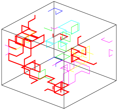
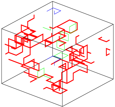
Figure 2: (Color online) Vortex-loop networks for the “stochastic” definition with $c=0.4$ (left) and the “maximal” definition with $c=1$ (right). Both networks are generated from the same $L=8$ lattice field configuration at the (thermodynamically) critical coupling $\beta_{c}=0.780\,08$. The different loops are distinguished by the color coding.

We can thus extract from each lattice configuration a set of vortex loops, which have been glued together by one of the connectivity definitions above. In Fig. 2 we show two possible vortex-loop networks for $c=0.4$ and $c=1$ generated out of the same lattice configuration.

For each loop in the network, we measure the following observables:

• “Mass”, ${\cal O}_{\rm mass}$: The “mass” of a vortex loop is the number of line elements $*l_{\mu,n}$ of the loop, i.e., simply its length $l_{\rm loop}$ normalized by the volume

  $$\mathcal{O}_{\rm{mass}}\equiv l_{\rm loop}/N~{}.$$ (8)

  By summing over all loops of a configuration we recover of course the vortex density (7),

  $$\sum_{\rm loops}{O}_{\rm{mass}}=v~{}.$$ (9)

  For the percolation analysis the mass of the longest loop $\mathcal{O}_{\rm{mass}}^{\rm max}$ in each vortex network is recorded, which usually serves as a measure of the percolation strength (behaving similarly to a magnetization). stauffer

• “Volume”, ${\cal O}_{\rm vol}$: For each vortex loop, first the smallest rectangular box is determined that contains the whole loop. This value is then normalized by the volume of the lattice. A vortex loop spread over an extent $l_{x}$, $l_{y}$, and $l_{z}$ thus results in

  $$\mathcal{O}_{\rm{vol}}=(l_{x}\times l_{y}\times l_{z})/N~{}.$$ (10)

  For each lattice configuration, we record the maximal “volume” $\mathcal{O}_{\rm{vol}}^{\rm max}$, which may be taken as an alternative definition of the percolation strength.

• “Extent” of a vortex loop in 1, 2, or 3 dimensions, ${\cal O}_{\rm 1D},{\cal O}_{\rm 2D},$ and ${\cal O}_{\rm 3D}$: This means simply to project the loop onto the three axes and record whether the projection covers the whole axis, or to be more concrete, whether one finds a vortex-line element of the loop in all planes perpendicular to the eyed axis. If there is a loop fulfilling this requirement, then this loop is percolating and we record $1$ in the time series of measurements; if not, a value of $0$ is stored. This quantity can thus be interpreted as percolation probability stauffer which (behaving similarly to a Binder parameter) is a convenient quantity for locating the percolation threshold $\beta_{p}$.

• “Susceptibilities,” $\chi_{i}$: For the vortex-line density $v$ and any of the observables ${\cal O}_{i}$ defined above ($i=$ “mass,” “vol,” “1D,” …), one can use its variance to define the associated susceptibility,

  $$\chi_{i}=N(\langle{\cal O}_{i}^{2}\rangle-\langle{\cal O}_{i}\rangle^{2})~{},$$ (11)

  which is expected to signal critical fluctuations.

• “Line tension,” $\theta$: On general grounds the loop-length distribution $P(l_{\rm loop})$ is expected to have the following form: adriaan

  $$P(l_{\rm loop})\sim l_{\rm loop}^{-\tau}\exp{(-l_{\rm loop}\theta)}~{},$$ (12)

  where the Fisher exponent $\tau$ is given in terms of the fractal dimension $D$ of the loops by

  $$\tau=\frac{d}{D}+1~{}.$$ (13)

  For a three-dimensional ($d=3$) (noninteracting) Brownian random walk with $D=2$ this leads to $\tau=5/2$, while $\tau>5/2$ for self-avoiding and $\tau<5/2$ for self-seeking lines, respectively. The parameter $\theta$ is the line tension which vanishes according to kajantie

  $$\theta=|\beta-\beta_{p}|^{\gamma_{\theta}}~{},$$ (14)

  where $\beta_{p}$ is the percolation threshold of the random walk and $\gamma_{\theta}\equiv 1/\sigma_{\theta}$ the second independent percolation exponent. stauffer

III Simulation and Results

Let us now turn to the description of the Monte Carlo update procedures used by us. We employed the single-cluster algorithm wolff to update the direction of the field, hasen similar to simulations of the $XY$ spin model. WJ_XY The modulus of $\psi$ is updated with a Metropolis algorithm. Metro ; WJ_review Here some care is necessary to treat the measure in Eq. (4) properly (see Ref. ebwj_prl, ). One sweep consisted of $N$ spin flips with the Metropolis algorithm and $N_{\rm sc}$ single-cluster updates. For all simulations the number of cluster updates was chosen roughly proportional to the linear lattice size, $N_{\rm sc}\simeq L$, a standard choice for three-dimensional systems as suggested by a simple finite-size scaling (FSS) argument. We performed simulations for lattices with linear lattice size $L=6$ – $10,12,14,16,18,20,22,24,26,28,32,36,$ and $40$, respectively, subject to periodic boundary conditions. After an initial equilibration time of $20\,000$ sweeps we took about $100\,000$ measurements, with ten sweeps between the measurements. All error bars are computed with the Jackknife method. Jack

Table 1: The critical exponents of the 3D $XY$ model universality class as reported in Ref. hasen2, and the correction-to-scaling exponent $\omega$ of Ref. hasen, .

$\alpha$	$\beta$	$\gamma$	$\delta$	$\eta$	$\nu$	$\omega$
$-0.0146(8)$	0.3485(2)	1.3177(5)	4.780(2)	0.0380(4)	0.67155(27)	0.79(2)

In order to be able to compare standard, thermodynamically obtained results (working directly with the original field variables) with the percolative treatment of the geometrically defined vortex-loop networks considered here, we used the same value for the parameter $\sigma=1.5$ as in Ref. ebwj_PRB, for which we determined by means of standard FSS analyses a critical coupling of

$$\beta_{c}=0.780\,08(4)~{}.$$ (15)

Focussing here on the vortex loops, we performed new simulations at this thermodynamically determined critical value, $\beta=0.780\,08$, as well as additional simulations at $\beta=0.79$, $0.80$, and $0.81$. The latter $\beta$ values were necessary because of the spreading of the pseudocritical points of the vortex loop related quantities. As previously we recorded the time series of the energy $H$, the magnetization $M$, the mean modulus $\overline{|\psi|}$, and the mean-square amplitude$|\psi|^{2}$, as well as the helicity modulus $\Gamma_{\mu}$ and the vortex-line density $v$. In the present simulations, however, we saved in addition also the field configurations in each measurement. This enabled us to perform the time consuming analyses of the vortex-loop networks after finishing the simulations and thus to systematically vary the connectivity parameter $c$ of the knots.

The FSS ansatz for the pseudocritical inverse temperatures $\beta_{i}(L)$, defined as the points where the various $\chi_{i}$ obtain their maxima, is taken as usual as

$$\beta_{i}(L)=\beta_{i,c}+c_{1}L^{-1/\nu}+c_{2}L^{-1/\nu-\omega}+\dots~{},$$ (16)

where $\beta_{i,c}$ denotes the infinite-volume limit, and $\nu$ and $\omega$ are the correlation length and confluent correction critical exponents, respectively. Here we have deliberately retained the subscript $i$ on $\beta_{i,c}$.

Let us start with the susceptibility $\chi_{v}$ of the vortex-line density. Note that this quantity, while also being expressed entirely in terms of vortex elements, plays a special role in that it is locally defined, i.e., does not require a decomposition into individual vortex loops (which, in fact, is the time-consuming part of the vortex-network analysis). Assuming the $XY$ model values for $\nu$ and $\omega$ compiled in Table 1, which are taken from Refs. hasen, and hasen2, , and fitting only the coefficients $\beta_{i,c}$ and $c_{i}$, we arrive at the estimate

$$\beta_{v,c}=0.7797(14)~{}$$ (17)

with a goodness-of-fit parameter $Q=0.20$. This value is perfectly consistent with the previously obtained “thermodynamic” result (15), derived from FSS of the magnetic susceptibility and various (logarithmic) derivatives of the magnetization. On the basis of this result, it would be indeed tempting to conclude that the phase transition in the three-dimensional complex Ginzburg-Landau field theory can be explained in terms of vortex-line proliferation. antunes1 ; antunes2 As pointed out above, however, the vortex-line density $v$ does not depend on the connectivity of the vortex network and therefore does not probe its percolation properties. In fact, $v$ behaves similar to the energy and the associated susceptibility $\chi_{v}$ similar to the specific heat, so that the good agreement between Eqs. (15) and (17) is a priori to be expected.

To develop a purely geometric picture of the mechanism governing this transition, one should thus be more ambitious and also consider the various quantities $\mathcal{O}_{i}$ introduced above that focus on the percolative properties of the vortex-loop network. As an example for the various susceptibilities considered, we show in Fig. 3 the susceptibility $\chi_{\rm 3D}$ of ${\cal O}_{\rm 3D}$ for $c=0$ and $c=1$. The resulting scaling behavior of the maxima locations $\beta_{\rm 3D}(L)$ is depicted in Fig. 4, where the lines indicate fits according to Eq. (16) with exponents fixed again according to Table 1. We obtain $\beta_{{\rm 3D},c}=0.7824(1)$ with $\chi^{2}/{\rm dof}=1.14$ $(Q=0.32,L\geq 8)$ for $c=0$ and $\beta_{{\rm 3D},c}=0.8042(4)$ with $\chi^{2}/{\rm dof}=0.75$ $(Q=0.58,L\geq 20)$ for $c=1$. While for the “stochastic” rule with $c=0$ the infinite-volume limit of $\beta_{\rm 3D}(L)$ is at least close to $\beta_{c}$, it is clearly significantly larger than $\beta_{c}$ for the fully knotted vortex networks with $c=1$.

By repeating the fits for all vortex-network observables and the parameter $c$ between 0 and 1 in steps of 0.1, we find the results collected in Tables 2 and 3. To check the stability of the fit results we performed fits with different lower bounds of the fit range $L_{\rm min}$, while the upper bound was always our largest lattice size $L=40$. For all observables, except for ${\cal O}_{\rm 3D}$, we found a weak dependence of $\beta_{i,c}$ on the fit range. For all five observables we see that the location of the infinite-volume limit $\beta_{i,c}$ does depend on the connectivity parameter $c$ used in constructing the vortex loops in a statistically significant way. With decreasing $c$, the infinite-volume extrapolations come closer toward the thermodynamical critical value (15), but even for $c=0$ they clearly do not coincide.

As in Ref. kajantie, we found that the percolation points $\beta_{i,c}$ of ${\cal O}_{i}$ satisfy some inequalities. Because each lattice cube has three plaquettes, ${\cal O}_{\rm vol}\geq{\cal O}_{\rm mass}/3$, and it is plausible that $\langle{\cal O}_{\rm 1D}\rangle\geq\langle{\cal O}_{\rm 2D}\rangle\geq\langle{\cal O}_{\rm 3D}\rangle$. The first relation implies

$$\beta_{{\rm vol},c}\geq\beta_{{\rm mass},c}~{}.$$ (18)

Our results collected in Table 2 are consistent with this inequality. In addition to this inequality the authors of Ref. kajantie, also conjectured that $\beta_{{\rm vol},c}=\beta_{{\rm 3D},c}=\beta_{{\rm 1D},c}$. Our numerical data show that $\beta_{{\rm vol},c}\approx\beta_{{\rm 1D},c}$, but the other percolation points satisfy only the following inequalities:

$$\beta_{{\rm vol},c}\approx\beta_{{\rm 1D},c}\geq\beta_{{\rm 2D},c}\geq\beta_{{\rm 3D},c}~{},$$ (19)

cf. Table 3. The reason for this are possibly different corrections to scaling for the different observables. In the infinite-volume limit all definitions should lead to the same critical point.

These findings are reminiscent of the percolation behavior of, say, Ising (minority) spin droplets of like spins which are known to percolate in three dimensions already below the transition temperature, i.e., $\beta_{p}>\beta_{c}$ as for the vortex-loop observables. Only by breaking bonds between like spins with a certain temperature dependent probability $p_{b}^{\rm FK}$ ($=\exp(-2\beta)$), one can tune the thus defined Fortuin-Kasteleyn (FK) clusters to percolate at $\beta_{c}$. With any other non-FK probability $0<p_{b}<p_{b}^{\rm FK}$ for breaking bonds between like spins it is conceivable that the associated percolation point would be located somewhere between $\beta_{p}$ of the geometrical droplets and the thermodynamical (or, equivalently, FK) critical point $\beta_{c}$ (for $p_{b}>p_{b}^{\rm FK}$ the percolation transition may even vanish altogether). By analogy, our connectivity parameter $c$ seems to play a similar role for the vortex-loop network as $p_{b}$ for the spin droplets. However, due to the missing analog to the FK representation of the Ising model, in the present case of the vortex-loop network, it is not easy to guess a suitable temperature dependence of the parameter $c$ and we hence eluded to using a systematic variation of $c$ in small constant increments. The other important difference to the case of Ising droplets is of course the long-range interaction between vortex-line elements which certainly puts the sketched analogy to Ising droplets on quite an uncertain and speculative footing.

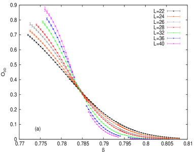
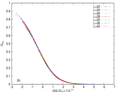
Figure 5: (Color online) (a) ${\cal O}_{\rm 3D}$ as a function of inverse temperature $\beta=1/T$ for $c=0$. (b) Rescaled data with $\nu$ fixed at the 3D $XY$ model value (cf. Table 1) and choosing $\beta_{c}({\cal O}_{\rm 3D})=0.7842$ to be the location of the crossing point in (a) for the best data collapse.

With these remarks in mind we nevertheless performed tests whether at least for $c=0$ the critical behavior of the vortex-loop network may consistently be described by the three-dimensional $XY$ model universality class. As an example for a quantity that is a priori expected to behave as a percolation probability we picked again the quantity $\mathcal{O}_{\rm 3D}$ for which the susceptibility was already shown in Fig. 3. As is demonstrated in Fig. 5(a) for the case $c=0$, by plotting the raw data of $\mathcal{O}_{\rm 3D}$ as a function of $\beta$ for the various lattice sizes, one obtains a clear crossing point so that the interpretation of $\mathcal{O}_{\rm 3D}$ as percolation probability is nicely confirmed. To test the scaling behavior we rescaled the raw data in the FSS master plot shown in Fig. 5(b), where the critical exponent $\nu$ has the $XY$ model value given in Table 1 and $\beta_{c}(\mathcal{O}_{\rm 3D})=0.7842$ was independently determined by optimizing the data collapse, i.e., virtually this is the location of the crossing point in Fig. 5(a). The collapse turns out to be quite sharp which we explicitly judged by comparison with similar plots for standard bond and site percolation (using there the proper percolation exponent, of course). For $c>0$ we found also a sharp data collapse, but for a monotonically increasing exponent $\nu$, which is for large $c$ values compatible with the percolation critical exponent $\nu=0.8765(16)$ on a three-dimensional simple cubic lattice. ballesteros One should keep in mind, however, that neither $\beta_{{\rm 3D},c}$ as extrapolated from the susceptibility peaks nor the estimate obtained from the crossing point in Fig. 5(a) is compatible with $\beta_{c}$.

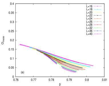
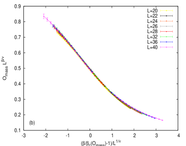
Figure 6: (Color online) (a) Mass of vortex loops as a function of inverse temperature $\beta=1/T$ for $c=0$. (b) Rescaled data assuming 3D $XY$ model critical exponents (cf. Table 1) and adjusting $\beta_{c}({\cal O}_{\rm mass})=0.782\,75$ for the best data collapse.

Next we looked at ${\cal O}_{\rm mass}$ which a priori is expected to behave like a percolation strength, that is similarly to the magnetization with an inverted $\beta$ axis. The plot of the raw data for $c=0$ as a function of $\beta$ in Fig. 6(a) indeed seems to confirm this expectation. To test the scaling properties we show in Fig. 6(b) the corresponding FSS master plot, where the critical exponents $\nu$ and $\beta$ are again fixed to their $XY$ model values (cf. Table 1) and $\beta_{c}({\cal O}_{\rm mass})=0.782\,75$ was determined by optimizing the data collapse. Also this collapse is comparatively sharp. Even though the thus obtained value for $\beta_{c}({\cal O}_{\rm mass})$ is consistent within error bars with the FSS value in Table 2 obtained from the susceptibility maxima locations (but even further away from $\beta_{c}$), we found a visible spread of the rescaled curves when the latter value was used and kept fixed. Similarly, assuming both $XY$ model exponents and $\beta_{c}({\cal O}_{\rm mass})=\beta_{c}$ does not produce a satisfactory data collapse. Thus for both observables, $\mathcal{O}_{\rm 3D}$ and ${\cal O}_{\rm mass}$, we obtain nice FSS scaling plots at $c=0$ compatible with $XY$ model critical exponents, but a “wrong” critical coupling.

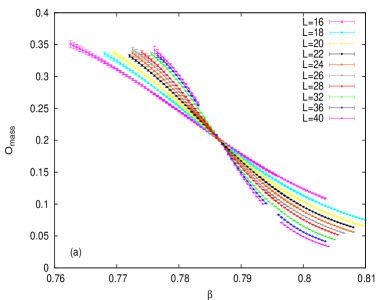
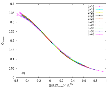
Figure 7: (Color online) Similar plot as in Fig. 6 for $c=0.4$. Here both $\beta_{c}({\cal O}_{\rm mass})=0.786\,46$ and $\nu=0.98$ are adjusted to achieve a good data collapse. Note that in contrast to Fig. 6(b), the $y$ axis in (b) is not rescaled.

Surprisingly, when using $c\neq 0$ for constructing the vortex loops, ${\cal O}_{\rm mass}$ shows a completely different behavior. As example, we show in Fig. 7 our data for the case $c=0.4$. Already by looking at the raw data in Fig. 7(a), it is obvious that, for $c\neq 0$, the mass of vortex loops no longer behaves as a percolation strength (i.e., magnetization); rather it resembles pretty much the percolation probability ${\cal O}_{\rm 3D}$. From the crossing point of the curves we get $\beta({\cal O}_{\rm mass})=0.786\,46$. Using this value we get in the FSS master plot shown in Fig. 7(b) a nice data collapse for $\nu=0.98$, but in contrast to the $c=0$ case now only when the $y$ axis is not rescaled. We repeated this analysis for all values $c>0$ and found a monotonically increasing exponent $\nu$ from $\nu\approx 0.74$ for $c=0.1$ to $\nu\approx 1.82$ for $c=1.0$, which appears quite nonsensical. A precise determination of the critical exponents as a function of $c$ was not our aim here and anyway, due to the rather small lattice sizes studied, also not feasible. Still, this strange behavior clearly calls for an explanation.

The variance definition (11) of the susceptibilities studied so far is quite unusual in percolation theory. We have therefore also investigated the standard percolation definition for the average loop size $\chi_{l_{\rm loop}}$ (as seen at a given link of the lattice) which is expected to scale as the variances defined above. In terms of the loop-length distribution $P(l_{\rm loop})$ it is given as stauffer

$$\chi_{L}=\frac{\sum^{\prime}_{\rm loop}l_{\rm loop}^{2}P(l_{\rm loop})}{\sum^{\prime}_{\rm loop}l_{\rm loop}P(l_{\rm loop})}~{},$$ (20)

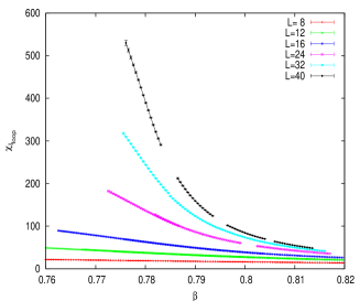
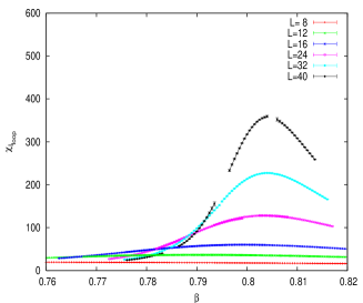
Figure 8: (Color online) Average loop size $\chi_{l_{\rm loop}}$ as a function of inverse temperature $\beta=1/T$ for $c=0$, $0.2$, and $1$ (from left to right).

where the prime on the sum is to indicate that we discard in each measurement the percolating loop according to the criterion $\mathcal{O}_{\rm 3D}$. For this observable we also found a clear displacement between the maxima for different values of the connectivity parameter $c$ and the thermodynamic transition point. Unfortunately, the reweighting range for $c=0$ was too narrow for this observable to allow more detailed analyses, see Fig. 8. For $c>0$ the location of the pseudocritical points of the average loop size behave similar to the susceptibilities as defined in Eq. (11) and lead to slightly higher $\beta_{c}$ values than the thermodynamic one.

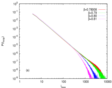
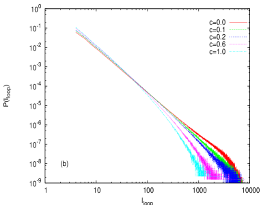
Figure 9: (Color online) Loop-length distribution $P(l_{\rm loop})$ for our largest lattice ($L=40$) as a function of the loop length. (a) The “stochastic” rule ($c=0$) for various temperatures. (b) Behavior at the thermodynamic critical point $\beta=0.780\,08$ for various values of the connectivity parameter $c$. At $c\approx 0.1$ the decay changes from exponential to algebraic implying that the vortex-line tension $\theta$ vanishes.

Finally, in Fig. 9(a) we show the loop-length distribution $P(l_{\rm loop})$ (without the largest loop) as a function of the loop length $l_{\rm loop}$ for the “stochastic” rule ($c=0$) for various temperatures and $L=40$. From Eq. (12) one expects that the decay changes from exponential to algebraic at $\beta_{c}$, because of the vanishing of the vortex-line tension $\theta$. Also from this analysis we found that the percolation transition takes place at a slightly higher $\beta$ value than the thermodynamic one. We performed fits according to $P(l_{\rm loop})\sim l_{\rm loop}^{-\tau}$ and found the best results for $\beta=0.79$ where $\tau\approx 2.2<5/2$, see Table 4. We want to note that this $\beta$ value is for our largest lattice and we only examined the loop-length distributions at the $\beta$ values used for the simulation. To determine the percolation transition and also the line tension with the help of the loop-length distributions one would need a finer temperature spacing. At $\beta_{c}$ of the thermodynamic transition we looked at the change of the decay of the distributions as a function of the connectivity parameter $c$ for $L=40$, see Fig. 9(b). Here we found the best agreement with an algebraic decay for $c=0.1$ with $\tau=2.348(1)$ and $\chi^{2}/{\rm dof}=2.9$. From this observation and the fact that we found a pronounced peak for the largest loops in the distribution at $c=0.1$ and no peak at $c=0.0$, we conclude that the line tension vanishes close to $c=0.0$.

IV Conclusion and Outlook

In this paper we have found for the three-dimensional complex Ginzburg-Landau field theory that the geometrically defined percolation transition of the vortex-loop network is close to the thermodynamic phase transition point, but does not coincide with it for any connectivity definition we have studied. Our results for the connectivity parameter $c\in[0,1]$ extend the claim of Ref. kajantie, for the three-dimensional $XY$ spin model that neither the “maximal” ($c=1$) nor the “stochastic” rule ($c=0$) used for constructing macroscopic vortex loops does reflect the properties of the true phase transition in a strict sense. sudbo1 Nevertheless it may be possible to bring the percolation transition closer to the thermodynamic one by using different vortex-loop network definitions, e.g., using a temperature-dependent or a size-dependent connectivity parameter in analogy to the Fortuin-Kasteleyn definition for spin clusters. To verify this presumption would be an interesting future project, but thereby one should first investigate the $XY$ model which is much less CPU time-consuming.

V Acknowledgments

We would like to thank Adriaan Schakel for many useful discussions. Disorder: from membranes to quantum gravity” for a postdoctoral grant. Financial support by the Deutsche Forschungsgemeinschaft (DFG) under grant No. JA 483/17-3 and the German-Israel-Foundation (GIF) under contract No. I-653-181.14/1999 is also gratefully acknowledged.

Table 2: FSS fits according to Eq. (16) in the range $L_{\rm min}$ to $L_{\rm max}=40$ for the mass and volume order parameter of the vortex loops for various values of $c$ ($c=1$: maximally knotted), with exponents $\nu$ and $\omega$ fixed according to Table 1. The thermodynamic transition is at $\beta_{c}=0.780\,08(4)$ (Ref. ebwj_PRB, ).

	${\cal O}_{\rm mass}$				${\cal O}_{\rm vol}$
$c$	$\beta_{c}$	$L_{\rm min}$	$\chi^{2}/{\rm dof}$	$Q$	$\beta_{c}$	$L_{\rm min}$	$\chi^{2}/{\rm dof}$	$Q$
1.0	0.8017(8)	20	1.53	0.17	0.8072(4)	12	1.86	0.05
0.9	0.8016(6)	16	1.66	0.11	0.8048(3)	14	1.08	0.37
0.8	0.7996(9)	16	1.55	0.14	0.8028(3)	14	1.40	0.19
0.7	0.7976(5)	14	1.34	0.21	0.8005(4)	16	1.14	0.33
0.6	0.7970(5)	16	1.10	0.36	0.7995(5)	14	0.57	0.80
0.5	0.7954(6)	18	1.32	0.24	0.7963(3)	16	1.23	0.28
0.4	0.7912(5)	14	0.94	0.48	0.7938(4)	18	0.82	0.55
0.3	0.7887(9)	16	1.32	0.23	0.7924(4)	18	1.79	0.09
0.2	0.7856(3)	6	1.62	0.07	0.7907(4)	12	0.28	0.98
0.1	0.7834(4)	10	0.37	0.96	0.7875(2)	12	0.94	0.49
0.0	0.7811(39)	10	1.26	0.24	0.7834(3)	16	0.92	0.48

Table 3: Same as in Table 2 for the vortex parameters ${\cal O}_{\rm 1D}$, ${\cal O}_{\rm 2D}$, and ${\cal O}_{\rm 3D}$.

	${\cal O}_{\rm 1D}$				${\cal O}_{\rm 2D}$				${\cal O}_{\rm 3D}$
$c$	$\beta_{c}$	$L_{\rm min}$	$\chi^{2}/{\rm dof}$	$Q$	$\beta_{c}$	$L_{\rm min}$	$\chi^{2}/{\rm dof}$	$Q$	$\beta_{c}$	$L_{\rm min}$	$\chi^{2}/{\rm dof}$	$Q$
1.0	0.8066(5)	16	0.68	0.68	0.8051(3)	20	0.86	0.50	0.8042(4)	20	0.75	0.58
0.9	0.8048(3)	16	0.68	0.69	0.8032(3)	20	0.72	0.61	0.8027(3)	18	0.37	0.89
0.8	0.8030(2)	16	1.04	0.40	0.8027(4)	14	0.74	0.66	0.8009(2)	18	0.54	0.77
0.7	0.8011(2)	16	0.90	0.50	0.7999(3)	18	1.29	0.26	0.7988(2)	18	0.61	0.72
0.6	0.7992(3)	16	1.67	0.11	0.7976(2)	18	0.44	0.85	0.7968(2)	18	1.20	0.30
0.5	0.7966(3)	16	0.94	0.47	0.7953(2)	18	0.42	0.86	0.7953(2)	18	0.72	0.67
0.4	0.7938(3)	20	1.18	0.32	0.7940(2)	14	1.10	0.36	0.7928(2)	12	0.35	0.96
0.3	0.7919(2)	18	1.11	0.35	0.7915(3)	16	0.66	0.71	0.79037(5)	6	0.54	0.91
0.2	0.7907(2)	12	1.10	0.37	0.7890(2)	16	0.68	0.69	0.7881(1)	6	0.92	0.53
0.1	0.7868(3)	18	1.38	0.21	0.7861(2)	18	0.49	0.81	0.7857(2)	6	0.60	0.86
0.0	0.7837(2)	12	1.84	0.08	0.7824(5)	18	0.28	0.94	0.7824(1)	8	1.14	0.32

Table 4: Results for the Fisher exponent $\tau$ for the “stochastic” definition ($c=0$) at three inverse temperatures $\beta=1/T$, assuming an algebraic decay of the loop-length distribution close to criticality.

$\beta$	fit range	$\tau$	$\chi^{2}/{\rm dof}$
0.78008	$20-500$	2.261(1)	3.1
0.79	$20-800$	2.201(1)	1.4
0.80	$20-500$	2.275(1)	26

Figure 3: Susceptibility of ${\cal O}_{\rm 3D}$ as a function of inverse temperature $\beta=1/T$ for (a) the “stochastic” rule ($c=0$) and (b) the “maximal” rule ($c=1$).

Figure 4: Location of the percolation thresholds determined from the maximum of susceptibility of ${\cal O}_{\rm 3D}$ for $c=0$ and $c=1$ as a function of (a) $L$ and (b) $L^{-1/\nu}$, respectively. The lines indicate fits according to Eq. (16) with $\nu$ and $\omega$ fixed according to Table 1. The horizontal dashed line shows the thermodynamically determined critical coupling $\beta_{c}=0.780\,08(4)$.

References

- (1) V.L. Berezinskii, Zh. Eksp. Teor. Fiz. 61, 1144 (1971) [Sov. Phys. JETP 34, 610 (1972)].
- (2) J.M. Kosterlitz and D.J. Thouless, J. Phys. C 6, 1181 (1973).
- (3) T. Banks, R. Myerson, and J. Kogut, Nucl. Phys. B 129, 493 (1977).
- (4) D. Stauffer and A. Aharony, Introduction to Percolation Theory, 2nd ed. (Taylor and Francis, London, 1994).
- (5) K. Kajantie, M. Laine, T. Neuhaus, A. Rajantie, and K. Rummukainen, Phys. Lett. B 482, 114 (2000).
- (6) P.W. Kasteleyn and C.M. Fortuin, J. Phys. Soc. of Japan 26 (Suppl.), 11 (1969); C.M. Fortuin and P. W. Kasteleyn, Physica 57, 536 (1972); C.M. Fortuin, ibid. 58, 393 (1972); C.M. Fortuin, ibid. 59, 545 (1972).
- (7) A. Coniglio and W. Klein, J. Phys. A 13, 2775 (1980).
- (8) S. Fortunato, J. Phys. A 36, 4269 (2003).
- (9) W. Janke and A.M.J. Schakel, Nucl. Phys. B 700, 385 (2004).
- (10) P. Curty and H. Beck, Phys. Rev. Lett. 85, 796 (2000).
- (11) W. Janke, Phys. Lett. A 148, 306 (1990).
- (12) A.M.J. Schakel, Phys. Rev. E 63, 026115 (2001).
- (13) U. Wolff, Phys. Rev. Lett. 62, 361 (1989); Nucl. Phys. B 322, 759 (1989).
- (14) M. Hasenbusch and T. Török, J. Phys. A 32, 6361 (1999).
- (15) N. Metropolis, A.W. Rosenbluth, M.N. Rosenbluth, A.H. Teller, and E. Teller, J. Chem. Phys. 21, 1087 (1953).
- (16) W. Janke, Math. Comput. Simul. 47, 329 (1998); and in: Computational Physics: Selected Methods – Simple Exercises – Serious Applications, eds. K.H. Hoffmann and M. Schreiber (Springer, Berlin, 1996); p. 10.
- (17) E. Bittner and W. Janke, Phys. Rev. Lett. 89, 130201 (2002).
- (18) B. Efron, The Jackknife, the Bootstrap and Other Resampling Plans (Society for Industrial and Applied Mathematics [SIAM], Philadelphia, 1982).
- (19) E. Bittner and W. Janke, Phys. Rev. B 71, 024512 (2005)
- (20) M. Campostrini, M. Hasenbusch, A. Pelissetto, P. Rossi, and E. Vicari, Phys. Rev. B 63, 214503 (2001).
- (21) N.D. Antunes, L.M.A. Bettencourt, and M. Hindmarsh, Phys. Rev. Lett. 80, 908 (1998).
- (22) N.D. Antunes and L.M.A. Bettencourt, Phys. Rev. Lett. 81, 3083 (1998).
- (23) H.G. Ballesteros, L.A. Fernandez, V. Martin-Mayor, A. Munoz-Sudupe, G. Parisi, and J. J. Ruiz-Lorenzo, J. Phys. A 32, 1 (1999).
- (24) Similar results for the and the Ginzburg-Landau model have been found for a slightly different definition of (cf. ) by A.K. Nguyen and A. Sudbø, Phys. Rev. B 60, 15307 (1999). We have some doubt about the correctness of the results for the Ginzburg-Landau model, because it seems that the authors did not properly take into account the Jacobian factor which emerges from the complex measure of the partition function when transforming the field representation from Cartesian to polar coordinates. For detailed discussions of this point, see Ref. ebwj_prl, .