Phase Diagram of the Bose-Hubbard Model with $\mathcal{T}_{3}$ symmetry

Abstract

In this paper we study the quantum phase transition between the Insulating and the globally coherent superfluid phases in the Bose-Hubbard model with $\mathcal{T}_{3}$ structure, the “dice lattice”. Even in the absence of any frustration the superfluid phase is characterized by modulation of the order parameter on the different sublattices of the $\mathcal{T}_{3}$ structure. The zero-temperature critical point as a function of a magnetic field shows the characteristic “butterfly” form. At fully frustration the superfluid region is strongly suppressed. In addition, due to the existence of the Aharonov-Bohm cages at $f=1/2$, we find evidence for the existence of an intermediate insulating phase characterized by a zero superfluid stiffness but finite compressibility. In this intermediate phase bosons are localized due to the external frustration and the topology of the $\mathcal{T}_{3}$ lattice. We name this new phase the Aharonov-Bohm (AB) insulator. In the presence of charge frustration the phase diagram acquires the typical lobe-structure. The form and hierarchy of the Mott insulating states with fractional fillings, is dictated by the particular topology of the $\mathcal{T}_{3}$ lattice. The results presented in this paper were obtained by a variety of analytical methods: mean-field and variational techniques to approach the phase boundary from the superconducting side, and a strongly coupled expansion appropriate for the Mott insulating region. In addition we performed Quantum Monte Carlo simulations of the corresponding (2+1)D XY model to corroborate the analytical calculations with a more accurate quantitative analysis. We finally discuss experimental realization of the $\mathcal{T}_{3}$ lattice both with optical lattices and with Josephson junction arrays.

I Introduction

The Bose-Hubbard (BH) model fisher89 is a paradigm model to study a variety of strongly correlated systems as superconducting films sondhi97 , Josephson junction arrays fazio01 and optical lattices jaksch98 ; greiner02 . This model predicts the existence of a zero-temperature phase transition from an insulating to a superfluid state which, by now, has received ample experimental confirmation. The BH model is characterized by two energy scales, an on-site repulsion energy between the bosons $U$ and an hopping energy $t$ which allows bosons to delocalize. At zero temperature and in the limit $U\gg t$ bosons are localized because of the strong local interactions. There is a gap in the spectrum for adding (subtracting) a particle, hence the compressibility vanishes. This phase is named the Mott insulator. In the opposite limit, $U\ll t$, bosons are delocalized and hence are in a superfluid phase. There is a direct transition between the Mott insulator and the superfluid state at a critical value of the ratio $t/U$. This Superfluid-Insulator (SI) transition has been extensively studied both theoretically and experimentally and we refer to Refs.  sondhi97, ; fazio01, ; jaksch98, ; greiner02, (and references therein) for an overview of its properties.

Magnetic frustration can be introduced in the BH-model by appropriately changing the phase factors associated to the hopping amplitudes. The presence of frustration leads to a number of interesting physical effects which has been explored both experimentally and theoretically. In Josephson arrays, where this is realized by applying an external magnetic field, frustration effects have been studied extensively in the past for both classical frustration and quantum systems fazio01 . Very recently a great interest in studying frustrated optical lattices has emerged as well jaksch03 ; sorensen05 ; polini05 ; osterloh05 . There are already theoretical proposals to generate the required phases factors by means of atoms with different internal states jaksch03 or by applying quadrupolar fields sorensen05 .

The interest in the properties of dice lattices sutherland86 has been stimulated by the work by Vidal et al. vidal98 on the existence of localization, the so called Aharonov-Bohm (AB) cages, in fully frustrated dice lattices without any kind of disorder. The existence of these cages is due to destructive interference along all paths that particles could walk on, when the phase shift around a rhombic plaquette is $\pi$. Following the original paper by Vidal et al., several experimental abilio99 ; naud01 ; serret03 and theoretical works korshunov02 ; doucot02 ; cataudella03 ; korshunov03 ; protopopov04 ; bercioux04 analyzed the properties of the AB cages. In the case of superconducting networks most of the attention has been devoted to classical arrays with the exception of Refs. doucot02, ; protopopov04, where a frustrated quantum quasi-one dimensional array were studied.

In quantum arrays (charge) frustration can also be induced by changing either the chemical potential (in optical lattices) or by means of a gate voltage (in Josephson junction arrays). This has the effect of changing the electrostatic energy needed to add/remove a boson on a given island. The phase diagram present a typical lobe-like structure fisher89 . Moreover, depending on the range of the interaction, it may also induce Wigner-like lattices of Cooper pairs commensurate with the underlying lattice bruder93 .

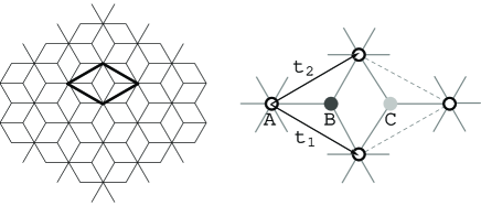
Figure 1: The $\mathcal{T}_{3}$ lattice: It consist of hubs (with six nearest neighbours) connected to rims (three nearest neighbours). The $\mathcal{T}_{3}$ structure is a Bravais lattice with a base inside the conventional unitary cell. The lattice vectors are $\mathbf{t_{1}}$ and $\mathbf{t_{2}}$. The basis is given by the sites A,B,C. Due to the fact that these sublattices are not self-connected and have different coordination numbers, we refer to this structure as tripartite. All rhombic plaquettes are identical, although differently oriented.

The aim of this work is to study the phase diagram of a Bose-Hubbard model on a $\mathcal{T}_{3}$ lattice (shown in Fig.1). We will consider both the cases of electric and magnetic frustration. The location and the properties of the phase diagram will be analyzed by a variety of approximate analytical methods (mean-field, variational Gutzwiller approach, strong coupling expansion) and by Monte Carlo simulations. The $\mathcal{T}_{3}$ lattice has been experimentally realized in Josephson arrays serret03 . In addition we show that it is possible to realize it experimentally also with optical lattices. Although the main properties of the phase diagram are common to both experimental realizations, there are some differences which are worth to be highlighted.

The plan of the paper is the following. In the next Section we will discuss the appropriate model for both the case of a Josephson junction array and optical lattices (Sec. II) and discuss in some detail how the $\mathcal{T}_{3}$ structure can be realized in an optical lattice (Sec. II.2). In the same Section we introduce the relevant notation to be used in the rest of the paper. A description of the various analytical approaches used to obtain the phase diagram will be given in Sec. III. The zero-temperature phase diagram, in the presence of magnetic and electric frustration, will then be described in Sec. IV. We first discuss the unfrustrated case and afterwards we consider the role of electric and magnetic frustration respectively. Due to the particular topology of the $\mathcal{T}_{3}$ lattice the superconducting phase is characterized, even at zero frustration, by a modulation of the order parameter on the different sublattices (i.e. hubs and rims), which indicates a different phase localization on islands depending on their coordination number. A uniform electrostatic field gives rise to a lobe structure in the phase diagram which is discussed for the $\mathcal{T}_{3}$ array in Sec. IV.2. The effect of a uniform external magnetic field, discussed in Sec. IV.3, may induce important qualitative changes in the phase diagram in the case of fully frustration. In particular we will provide evidences that there is an important signature of the Aharonov-Bohm cages in the quantum phase diagram. It seems that due to the AB cages a new phase intermediate between the Mott insulating and superfluid phases should appear. On varying the ratio between the hopping and the Coulomb energy the system undergoes two consecutive quantum phase transitions. At the first critical point there is a transition from a Mott insulator to a Aharonov-Bohm insulator. The stiffness vanishes in both phases but the compressibility is finite only in the Aharonov-Bohm insulator. At a second critical point the system goes into a superfluid phase. Most of the analysis is presented by using approximated analytical methods. These results will be checked against Monte Carlo simulations that we present in Sec. IV.4. Few details of the mapping of the model used in the simulation are reviewed in the Appendix A. The concluding remarks are summarized in Sec. V.

II Quantum Phase Model on a $\mathcal{T}_{3}$ array

Both Josephson arrays and optical lattices are experimental realizations of the Bose-Hubbard model

$$\mathcal{H} = \mathcal{H}_{U}+\mathcal{H}_{t}$$ (1)

$$= \frac{1}{2}\sum_{ij}(n_{i}-n_{0})\mathcal{U}_{i,j}(n_{i}-n_{0})$$

$$- \frac{\tilde{t}}{2}\sum_{<ij>}(b^{{\dagger}}_{i}b_{j}+h.c.)\;\;.$$

When the mean occupation ${\bar{n}}$ on each lattice site is large, one is allowed to introduce the phase operator $\varphi_{i}$ by approximating the boson annihilation operator on site $i$ by $b_{i}\simeq\sqrt{{\bar{n}}}~{}\exp{[\imath\varphi_{i}]}$. The density $n_{i}$ and phase $\varphi_{i}$ operators are canonically conjugate on each site

$$\left[n_{i},e^{\pm\imath\varphi_{j}}\right]=\pm\delta_{i,j}\,e^{\pm\imath\varphi_{i}}\,.$$ (2)

In the present work we will focus our attention on the quantum rotor version of the model in Eq.(1) that reads:

$$\mathcal{H} = \frac{1}{2}\sum_{ij}(n_{i}-n_{0})\mathcal{U}_{i,j}(n_{j}-n_{0})$$ (3)

$$- t\sum_{<ij>}\cos(\varphi_{i}-\varphi_{j}-A_{i,j})\;\;.$$

The first term on the r.h.s of Eq.(3) represents the repulsion between bosons ($\mathcal{U}_{i,j}$ depends on the range of the interaction and on its detailed form). The second term is due to the boson hopping ($t=\bar{n}\tilde{t}$ is the coupling strength) between neighboring sites (indicated with $\langle.\rangle$ in the summation). The gauge-invariant definition of the phase in presence of an external vector potential $\mathbf{A}$ and flux-per-plaquette $\Phi$ ($\Phi_{0}=h\,c/\,2\,e$ is the flux quantum) contains the term $A_{i,j}=\frac{2\pi}{\Phi_{0}}\int_{i}^{j}\mathbf{A}\cdot d\mathbf{l}\;.$ All the observables are function of the frustration parameter defined as

$$f=\frac{1}{\Phi_{0}}\int_{P}\mathbf{A}\cdot d\mathbf{l}=\frac{1}{2\pi}\sum_{P}\,A_{i,j}$$ (4)

where the line integral is performed over the elementary plaquette. Due to periodicity of the model it is sufficient to consider values of the frustration $0\leq f\leq 1/2$. Charge frustration is due to a non-integer value $n_{0}$. As for the magnetic frustration also in this case the properties will be periodic under the transformation $n_{0}\rightarrow n_{0}+1$. Due to the additional symmetry $n_{0}\rightarrow-n_{0}$ it is sufficient to consider value of the charge frustration $n_{0}$ in $[0,1/2]$. Differently from the magnetic frustration the value of $n=1/2$ does not necessarily correspond to fully (charge) frustration as this depends on the range of the interaction $\mathcal{U}_{i,j}$.

The $\mathcal{T}_{3}$ lattice sutherland86 is represented in Fig.1, the lines between the sites corresponds to those links where boson hopping is allowed. The $\mathcal{T}_{3}$ structure is not itself a Bravais lattice, but could be considered as a lattice with a base inside the conventional unitary cell (see Fig. 1) defined by the vectors

$$\mathbf{t_{1}} = \left(3/2;-\sqrt{3}/2\right)a$$

$$\mathbf{t_{2}} = \left(3/2;+\sqrt{3}/2\right)a\;\;.$$

where $a$ is the lattice constant. The lattice sites of the base are at positions

$$\mathbf{d_{A}}=\left(0;0\right)a\hskip 8.5359pt\mathbf{d_{B}}=\left(0;1\right)a\hskip 8.5359pt\mathbf{d_{C}}=\left(0;2\right)a\;\;.$$

The reciprocal lattice ($\mathbf{g_{a}}\cdot\mathbf{t_{b}}=2\pi\delta_{a,b}$) vectors are defined as

$$\mathbf{g_{1}} = \frac{2\pi}{a}\left(1/3;-\sqrt{3}/3\right)$$

$$\mathbf{g_{2}} = \frac{2\pi}{a}\left(1/3;+\sqrt{3}/3\right)\;\;.$$

In several situations it turns out to be more convenient to label the generic site $i$ by using the position of the cell $\mathbf{t}=n_{1}\mathbf{t_{1}}+n_{2}\mathbf{t_{2}}$ ($-N_{l}\leq n_{l}<N_{l}$) and the position within the cell $\alpha=A,B,C$. In the rest of the paper we either use the index $i$ or the pair of labels $(\mathbf{t},\alpha)$. A generic observable $W_{i}$ can be written henceforth as $W_{\alpha}(\mathbf{t})$. By imposing Born-Von Karman periodic boundary conditions its Fourier transform is given by

$$\widetilde{W}_{\alpha}(\mathbf{K})=\frac{1}{\sqrt{4N_{1}N_{2}}}\sum_{\mathbf{t}}W_{\alpha}(\mathbf{t})\ e^{-\imath\mathbf{K}\cdot\mathbf{t}}$$ (5)

with $\mathbf{K}=k_{1}\mathbf{g_{1}}+k_{2}\mathbf{g_{2}}$ in the first Brillouin zone.

It is also useful to introduce a connection matrix $\mathcal{T}$ whose entries are non-zero only for islands connected by the hopping. More precisely $T_{\alpha,\gamma}(\mathbf{t,t^{\prime}})=1$ if site $\alpha$ of cell $\mathbf{t}$ is connected by a line (see Fig.1) to site $\gamma$ of cell $\mathbf{t^{\prime}}$ and $T_{\alpha,\gamma}(\mathbf{t,t^{\prime}})=0$ otherwise. The local coordination number is thus defined as $z_{\alpha}=\sum_{\mathbf{t^{\prime}},\gamma}T_{\alpha,\gamma}(\mathbf{t,t^{\prime}})$. It is $z=6$ for the hubs (labelled by A) and $z=3$ for the rims (labelled by B and C). For later convenience we also define the matrix $\mathcal{P}$ with elements

$$P_{\alpha,\gamma}(\mathbf{t,t^{\prime}})\ =T_{\alpha,\gamma}(\mathbf{t^{\prime}-t})\ e^{\imath\mathbf{A}_{\alpha,\gamma}(\mathbf{t,t^{\prime}})}$$ (6)

which includes the link phase factors which appear if the system is frustrated. In the whole paper we fix $k_{B}=\hbar=c=1$.

In the next two subsections we give a brief description of the origin and characteristics of the coupling terms in the Hamiltonian of Eq.(3) both for Josephson and optical arrays. In addition we show how to realize optical lattices with $\mathcal{T}_{3}$ symmetry.

II.1 Josephson junction arrays

Since the first realization of a Josephson Junctions Array (JJA) IBM , these systems have been intensively studied as ideal model systems to explore a wealth of classical phenomena classical such as phase transitions, frustration effects, classical vortex dynamics and chaos. One of the most spectacular result was probably the experimental observation BKTexp of the Berezinskii-Kosterlitz-Thouless transition (BKT) BKTth . Indeed, well below the BCS transition temperature, and in the classical limit, JJAs are experimental realization of the XY model. For sufficiently small (submicron) and highly resistive (normal state resistance $R_{N}>R_{Q}=h/4e^{2}$) junctions quantum effect start to play an important role. In addition to the Josephson energy, which controls the Cooper pair tunnelling between neighboring grains, also the charging energy $e^{2}/2C$ ($C$ is the geometrical junction capacitance) becomes important.

Experiments on JJAs are performed well below the BCS critical temperature and thus each island is in the superconducting state. The only important dynamical variable is the phase $\varphi_{i}$ of the superconducting order parameter in each island, canonically conjugated to the number of extra Cooper pairs $n_{i}$ present on that island. In Eq.(3), the coupling constant $t$ equals the Josephson coupling. Hence the second term in Eq.(3) represent the Josephson energy. The first term is due to charging energy which can be evaluated by assuming that each island has a capacitance to the ground $C_{0}$ and each junction a geometrical capacitance $C$. The electrostatic interaction between the Cooper pairs is defined as

$$\mathcal{U}=2e^{2}\mathcal{C}^{-1}\;.$$ (7)

The capacitance matrix is given by

$$C_{i,j}=(C_{0}+z_{i}C)\,\delta_{i,j}-C\,T_{i,j}\;.$$ (8)

Since both the connection and the capacitance matrices depend only on the distance between the cells (and on the base index of both sites), their space dependence can be simplified to

$$C_{\alpha,\gamma}(\mathbf{t,t^{\prime}})=C_{\alpha,\gamma}(\mathbf{0,t^{\prime}-t})\equiv C_{\alpha,\gamma}(\mathbf{t^{\prime}-t})$$ (9)

An estimate of the range of the electrostatic interaction is given by mooij $\lambda\approx\sqrt{C/C_{0}}$. The charge frustration $n_{0}$, that we assume to be uniform, can be induced by an external (uniform) gate voltage $V_{0}=n_{0}/C_{0}$.

Due to the particular structure of the $\mathcal{T}_{3}$ lattice, the charging energy of a single (extra) Cooper pair placed on a given islands depends on that site being a rim or a hub as shown in Fig.2. As a consequence quantum fluctuations of the phase of the superconducting order parameter may be different in the two different cases (rims or hubs). We will see in Sec.IV.1 that this property is responsible for an additional modulation of the order parameter in the superconducting phase.

Figure 2: Electrostatic energy (in units of $U_{0}=e^{2}/2C_{0}$) required to put an extra Cooper pair (for zero external charge) on an hub (straight line) and on a rim (dashed) as a function of the reduced capacitance $C/C_{0}$

II.2 Optical lattices

Following the work of Jaksch et al. jaksch98 , optical lattices have been widely studied as concrete realization of the Bose-Hubbard model that is, as we saw, directly related to the quantum phase model studied in this paper. The experimental test of the SI transition greiner02 has finally opened the way to study strongly correlated phenomena in trapped cold atomic gases. Very recently, several works addressed the possibility to induce frustration in optical lattices jaksch03 ; sorensen05 ; polini05 ; osterloh05 . It is therefore appealing to test the properties of the $\mathcal{T}_{3}$ lattice also with optical lattices once it is known how to create $\mathcal{T}_{3}$ lattices by optical means.

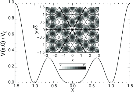
Figure 3: Optical potential with $\mathcal{T}_{3}$ symmetry generated by three counter-propagating laser beams. The inset shows the bidimensional contour plot while in the figure the details of the profile along a line connecting three sites (placed at positions $x=1$, $x=0$ and $x=-1$) is shown. The sites $x=-1,1$ are rims while the site at $x=0$ is a hub. Also here, as in the case of JJAs, the different form of the potential implies that the on-site energy $U_{0}$ is different for hubs and rims.

Here we propose an optical realization of a $\mathcal{T}_{3}$ structure by means of three counter-propagating pairs of laser beams. These beams divide the plane in six sectors of width $60$ (see the inset of Fig.3) and are linearly polarized such to have the electrical field in the $xy$ plane. They are identical in form, apart from rotations, and have wavelength equal to $\lambda=3/2\,a$ ($a$ is the lattice constant. Given a polarization of a pair of lasers on the $y$-axis $\vec{E_{1}}=(0,E_{y})$ the other two pairs are obtained by rotating $\vec{E_{1}}$ of $120$ and $-120$ around the $z$-axis. The square modulus of the total field gives rise to the desired optical potential as it is shown in Fig.3.

The form of the potential landscape also in this case imposes that the on-site repulsion may be different for hubs and rims. It is however diagonal

$$\mathcal{U}=U_{r}\;\mathcal{I}_{r}+U_{h}\;\mathcal{I}_{h}\;\;.$$ (10)

The subscript $h,r$ denotes the respectively the hub and rim sites and $\mathcal{I}_{h,r}$ are the projectors on the corresponding sublattices. In Eq.(3), now, the coupling $t$ describes the hopping amplitudes for bosons, $n_{0}$ is proportional to the chemical potential, $A_{ij}$ is the effective “magnetic frustration” that in this case may have several different origin depending on the scheme used. For simplicity we will always refer to $\vec{A}$ as to the vector potential and we will use the magnetic picture also for optical lattices.

III Analytic approaches

The SI transition has been studied by a variety of methods; here we apply several of them to understand the peculiarities that emerge in the phase diagram due to the $\mathcal{T}_{3}$ lattice structure. The results that derive from these approaches will be presented in the next section.

The location of the critical point depends on the exact form and the range of $\mathcal{U}_{i,j}$. This issue is particulary interesting when discussing the role of electric frustration. In the paper we address the dependence of the phase boundary on the range of the interaction in the mean-field approximation. The variational Gutzwiller ansatz and the strong coupling expansion will be analyzed only for the on-site case of Eq.(10). In the case of magnetic frustration the form of $\mathcal{U}_{i,j}$ leads only to quantitative changes so, also in this case, we discuss only the on-site case.

III.1 Mean field approach

The simplest possible approach to study the SI phase boundary consists in the evaluation of the superconducting order parameter, defined as

$$\psi_{i}=\langle e^{-\imath\varphi_{i}}\rangle\,,$$

by means of a mean-field approximation. By neglecting terms quadratic in the fluctuations around the mean field value, the hopping part of the Hamiltonian can be approximated as

$$\mathcal{H}_{t}^{(mf)}=-\frac{1}{2} t \sum_{i,j}e^{-\imath\varphi_{i}(\tau)}\ P_{i,j}\ \psi_{j}+h.c.$$

The order parameter is then determined via the self-consistency condition

$$\psi_{i}(\tau^{\prime})=\frac{\mbox{Tr}\left\{e^{\imath\varphi_{i}(\tau^{\prime})}\,e^{-\beta\,\mathcal{H}_{U}}\,\mathrm{T}_{\tau}\exp\left(\int_{0}^{\beta}\mathcal{H}_{t}^{(mf)}(\tau)\right)\right\}}{\mbox{Tr}\left\{e^{-\beta\,\mathcal{H}_{U}}\mathrm{T}_{\tau}\exp\left(\int_{0}^{\beta}\mathcal{H}_{t}^{(mf)}(\tau)\right)\right\}}\;.$$ (11)

In the previous equation, $\mathrm{T}_{\tau}$ is the time-ordering in imaginary time $\tau$ and $\beta=1/T$ . The $\tau$ dependence of the operators is given in the interaction representation $W(\tau)=e^{\tau\,\mathcal{H}_{U}}\,W\,e^{-\tau\,\mathcal{H}_{U}}$. For simplicity we already assumed the order parameter independent on the imaginary time. One can indeed verify that this is the case in the mean-field approximation. Close to the phase boundary the r.h.s. of Eq. 11 can be expanded in powers of the order parameter and the phase boundary is readily determined.

A central quantity in the determining the transition is the phase-phase correlator

$$G_{i,j}(\tau)=\langle\mathrm{T}_{\tau}e^{\imath\phi_{i}(\tau)}e^{-\imath\phi_{j}(0)}\rangle_{U}$$ (12)

where the average is performed with the charging part of the Hamiltonian only. Charge conservation imposes that the indexes $i,j$ are equal. The Matsubara transform at $T=0$ of the correlator reads

$$\widetilde{G}_{i,i}(\omega)=\int_{-\infty}^{\infty}G_{i,i}(\tau)e^{\imath\,\omega\,\tau}=\sum_{s=\pm}\frac{1}{\Delta E_{\alpha,s}-\imath s\omega}$$ (13)

where $\Delta E_{\alpha,\pm}$ are the excitation energies (for zero Josephson tunnelling) to create a particle (+) or a hole (-) on a site of the sublattice $\alpha$ where $i$ lies.

In the case of the $\mathcal{T}_{3}$ lattice considered here even at zero magnetic field the order parameter is not uniform. The tripartite nature of the lattice results in a vectorial mean field $\psi$ with one component for each sublattice. In the general case the linearized form of Eq.(11) can be rewritten as

$$\psi_{\alpha}(\mathbf{t})=\frac{t}{2}\sum_{\gamma}\sum_{\mathbf{t^{\prime}}}\widetilde{G}_{\alpha,\alpha}(0)P_{\alpha,\gamma}(\mathbf{t,t^{\prime}})\psi_{\gamma}(\mathbf{t^{\prime}})$$ (14)

that, due to the topology of the lattice is equivalent to

$$\psi_{\alpha}(\mathbf{t})=\frac{t^{2}}{4}\widetilde{G}_{A,A}(0)\,\widetilde{G}_{B,B}(0)\,\sum_{\gamma}\sum_{\mathbf{t^{\prime}}}P^{2}_{\alpha,\gamma}(\mathbf{t,t^{\prime}})\psi_{\gamma}(\mathbf{t^{\prime}})$$

The phase transition is identified with a non-trivial solution to this secular problem, i.e. one should determine $\pi_{max}$, the largest eigenvalue of $P$. This requirement translates in the following equation for the critical point

$$t_{cr}=2\frac{\pi_{max}^{-1}}{\sqrt{\widetilde{G}_{A,A}(0)\widetilde{G}_{B,B}(0)}}$$ (15)

In deriving the previous equation we used the fact that the sites $B$ and $C$ in the elementary cell (see Fig.1) have the same coordination number and therefore the phase-phase correlator is the same. In addition to the evaluation of the Matsubara transform at zero frequency of the phase correlator, one has to determine the eigenvalues of the gauge-link matrix $\mathcal{P}$. With a proper gauge choice it is possible to reduce this matrix to a block diagonal form. For rational values of the frustration, $f=p/q$, by choosing $\mathbf{A}~{}=~{}(x~{}-~{}\sqrt{3}~{}y)~{}\frac{2\Phi_{0}}{\sqrt{3}a^{2}}~{}f~{}\mathbf{\hat{y}}$, the magnetic phase factors $\mathbf{A}_{i,j}(\mathbf{t,t^{\prime}})$ (shown in Fig. 4) have a periodicity of $r\times 1$ elementary cells with $r=LCM(q,3)/3$. This implies that in the Fourier space (see Eq.(5)) the component $k_{2}$ is conserved and that $k_{1}$ is coupled only with the wavevectors $k_{1}^{(m)}=k_{1}+2\pi m/r$ ($m=0,...r-1$).

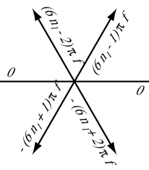
Figure 4: Magnetic phase pattern with the gauge choice $\mathbf{A}~{}=~{}(x~{}-~{}\sqrt{3}~{}y)~{}\frac{2\Phi_{0}}{\sqrt{3}a^{2}}~{}f~{}\mathbf{\hat{y}}$

.

The determination of $\pi_{max}$ is therefore reduced to the diagonalization of a $3r\times 3r$ matrix ($\widetilde{P}_{\alpha,\gamma}(k_{1})$ is $r\times r$)

$$\widetilde{\mathcal{P}}(k_{1},k_{2})=\delta_{k_{2},0}\left(\begin{array}[]{ccc}0&\widetilde{P}_{A,B}(k_{1})&\widetilde{P}_{A,C}(k_{1})\\ \widetilde{P}^{{\dagger}}_{A,B}(k_{1})&0&0\\ \widetilde{P}^{{\dagger}}_{A,C}(k_{1})&0&0\\ \end{array}\right)$$ (16)

with $(k_{1},k_{2})$ belonging to the reduced Brillouin zone $\mathbb{B}_{r}=\{0\leq k_{i}<2\pi/r\}$.

The matrix $\mathcal{P}$ has $r$ zero eigenvalues, and $r$ pairs of eigenvalues equal in absolute value given by the reduced secular equation

$$\left[\widetilde{P}_{1,2}(k_{1})\widetilde{P}^{{\dagger}}_{1,2}(k_{1})+\widetilde{P}_{1,3}(k_{1})\widetilde{P}^{{\dagger}}_{1,3}(k_{1})\right]\ \widetilde{v}_{1}=\pi^{2}\ \widetilde{v}_{1}$$

This simplification allows us to deal with $r\times r$ matrices instead of $q\times q$.

The inclusion of a finite range interaction, important only for Josephson arrays, leads to a richer lobe structure in presence of electrostatic frustration. The calculation of the lobes will be done within the mean field theory only.

III.2 Gutzwiller variational approach

A different approach, still mean-field in spirit, that allows to study the properties of the superconducting phase is the Gutzwiller variational ansatz adapted to the Bose-Hubbard model by Rokhsar and Kotliar rokhsar The idea is to construct a variational wave-function for the ground state starting from the knowledge of the wave-function in the absence of the interaction term $\mathcal{H}_{U}$ in the Hamiltonian. In this case, and in absence of magnetic frustration, the ground state has all the phases aligned along a fixed direction $\theta$. In the boson number representation it reads

$$|GS\rangle_{U=0}=\sum_{\{n_{i}\}}e^{\imath\sum_{i}n_{i}\theta}|\{n_{i}\}\rangle$$ (17)

A finite charging energy, tends to suppress the components of the state with large charge states, a variational state can then be constructed through the ansatz

$$|GS\rangle=\sum_{\{n_{i}\}}c_{n_{1},\cdots,n_{N}}|\{n_{i}\}\rangle$$ (18)

where

$$c_{\{n_{i}\}}=\frac{1}{\sqrt{N_{GS}}}e^{\imath\sum_{i}n_{i}\theta}e^{-\sum_{i}\ \frac{K_{i}}{2}(n_{i}-\overline{n}_{i})^{2}}\,.$$ (19)

In Eq.(19) $N_{GS}$ is a normalization factor and $K_{i}$ and $\overline{n}_{i}$ are variational parameter to be determined by minimizing the ground state energy. The Mott insulator is characterized by $K=\infty$, i.e. by perfect localization of the charges, $K=0$ is the limit of zero charging, a finite value of $K$ describes a superfluid phase where the phase coherence has been established albeit suppressed by quantum fluctuations.

III.3 Strong coupling perturbation theory

Both methods illustrated in Sections III.1 and III.2 are based on the analysis of the superconducting phase and on the determination of the phase boundary as the location of points where the superfluid order parameter vanishes. A complementary approach, which analyzes the phase boundary from the insulating side, was developed by Freericks and Monien freericks . The method was applied to the case of square and triangular lattices in Ref. niemeyer, for the Bose-Hubbard model and in Ref. kim, for the quantum rotor model. In this section we describe how to adapt the method to the $\mathcal{T}_{3}$ lattice. We will present the results of this analysis, particularly important for the fully frustrated case, in Sec. IV.3.

In the insulating phase the first excited state is separated by the ground state by a (Mott) gap. In the limit of vanishing hopping the gap is determined by the charging energy needed to place/remove an extra boson at a given lattice site. The presence of a finite hopping renormalizes the Mott gap which, at a given critical value, vanishes. The system becomes compressible, and the bosons, since are delocalized, will condense onto a superfluid phase. It is worth to emphasize that the identification of the SI boundary with the point at which the gap vanishes is possible as the bosons delocalize once the energy gap is zero. As we will see, in the case of $\mathcal{T}_{3}$ lattice the situation becomes more complex. In the presence of external magnetic frustration it may happen that though the Mott gap is zero, the states are localized and therefore the charges cannot Bose condense. In this cases between the Mott and superconducting region an additional compressible region (with zero superfluid stiffness) may appear. In order to keep the expressions as simple as possible we consider only the case of on-site interaction, though we allow a different $U$ for hubs and rims as in Eq.(10). The possible existence of such a phase, however, does not depend on the exact form of $\mathcal{U}_{i,j}$. The strong coupling expansion is particularly useful for $\mathcal{T}_{3}$ lattice as it may help in detecting, if it does exist, the intermediate phase.

In the strong-coupling approach of Freericks and Monien the task is to evaluate, by a perturbation expansion in $t/U$, the energy of the ground and the first excited state in order to determine the point where the gap vanishes. We denote the ground and first excited levels by $E_{M}^{gs}$ and $E_{M}^{exc}$ respectively. The choice of the starting point for the perturbation expansion is guided by the nature of the low-lying states of the charging Hamiltonian. When $n_{0}<1/2$ (and in zero-th order in $t/U$) the ground state of the electrostatic Hamiltonian is ($n_{i}=0\;\forall i$) and first excited level is given by a single extra charge localized on a site. Levels corresponding to charging a hub and a rim are nearly degenerate (i.e. $(U_{r}-U_{h})/(U_{r}+U_{h})\ll 1$, with the hub being lower in energy). As the strength of the hopping is increased, the insulating gap decreases. We would like to stress, and this is an important difference emerging from the $\mathcal{T}_{3}$ topology, i.e. the location of the extra charge (on a hub or a rim) requires a different energy. This in turn has important consequences in the structure of the perturbation expansion.

Up to the second-order in the tunnelling, the ground state energy at $n_{0}=0$ is given by

$$E_{M}^{gs}=-\frac{2\cdot 2N}{(U_{h}+U_{r})/2}\;\frac{t^{2}}{4}$$ (20)

where $N$ is the number of sites and $2N$ the number of hub-rim links in the lattice. Note that the first-order correction vanishes because the tunnelling term does not conserve local number of particles.

Due to nearly degeneracy of the excited levels, one is not allowed to perturb each of them independently but has to diagonalize the zeroth and the first order terms simultaneously. One has to diagonalize the following matrix:

$$\mathcal{Q}^{(1)}=\frac{1}{2}\mathcal{U}-\frac{t}{2}\mathcal{P}$$ (21)

This task can be reduced to the diagonalization of a $3r(f)\times 3r(f)$ matrix with a proper choice of the gauge (see Section III.1).

For example, the (degenerate) lowest eigenvalue at $f=1/2$ is

$$\left.Q_{min}^{(1)}\right|_{f=1/2}=\frac{U_{h}+U_{r}}{4}-\frac{1}{2}\,\sqrt{6t^{2}+\left(\frac{U_{r}-U_{h}}{2}\right)^{2}}$$ (22)

which reduces to $U/2-t\,\sqrt{6}/2$ in the case of perfectly degenerate charging energy. It must be stressed that all the energy bands are flat, independently of the values of the charging energies (it depends only on the peculiar $\mathcal{P}$ structure).

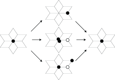
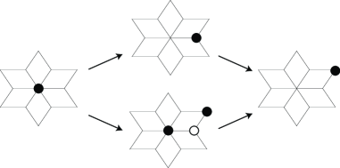
Figure 5: Intermediate charge states involved in the definition of Eq.(25). In the upper panel the contributions to the diagonal part are shown while in the lower panel there are the contributions to the off-diagonal part. The processes represented here are those contributing to the second order in the hopping amplitude. The black/white circles represent one extra +/- Cooper pair on a given site.

The second order perturbation term should be calculated on the lowest energy manifold: moreover only matrix elements between states of the same manifold are allowed. Nonetheless, it is simpler to write the different contributions in the usual basis of hub and rims (see Fig.(5)). The first excited state, to second order in tunnelling is given by

$$E_{M}^{(1)}=Q_{min}^{(1)}+\frac{t^{2}}{4}Q_{min}^{(2)}$$ (23)

where $\mathcal{Q}^{(2)}$ is the second order matrix and can be split into separate sub-matrices on different sub-lattices, i.e.

$$\mathcal{Q}^{(2)}=\mathcal{Q}^{(2)}_{h}\,\mathcal{I}_{h}+\mathcal{Q}^{(2)}_{r}\,\mathcal{I}_{r}$$ (24)

Such a decomposition is possible because after two tunnelling events the boson come back to the initial sublattice.

$$\mathcal{Q}(2)_{h} = z_{h}\frac{\mathcal{I}_{h}}{(U_{h}-U_{r})/2}+z_{h}\frac{\mathcal{I}_{h}}{\left(U_{h}-(4U_{h}+U_{r})\right)/2}$$ (25)

$$+ \left(2\cdot 2N-2z_{h}\right)\frac{\mathcal{I}_{h}}{(U_{h}-(2U_{h}+U_{r}))/2}$$

$$+ \frac{\mathcal{P}^{2}-z_{h}\mathcal{I}_{h}}{(U_{h}-U_{r})/2}+\frac{\mathcal{P}^{2}-z_{h}\mathcal{I}_{h}}{\left(U_{h}-(2U_{h}+U_{r})\right)/2}$$

($\mathcal{Q}(2)_{r}$ is defined in a similar way) where $\mathcal{I}_{h,r}$ are the projectors on the hub and rim sublattices. After some algebra and by changing basis to the one composed by the eigenvectors of Eq.(21), one gets the first excited energy level. The task is now to determine the location of points at which the gap, given by the difference of Eq.(23) and Eq.(20), vanishes. It is worth to stress that the thermodynamically divergent contributions wash out exactly their analogous in the ground state expression of Eq.20.

We discuss the results deriving from this approach in the next Section where we analyze the phase diagram.

IV Phase diagram

In order to keep the presentation as clear as possible we first discuss the main features of the phase diagram by means of the analytical approaches introduced before. We will then corroborate these results in a separate section by means of the Monte Carlo simulations.

The value of the critical Josephson coupling as a function of the range of the electrostatic interaction, in the absence of both electric and magnetic frustration is discussed first. The effect of frustration, either electric or magnetic will then be discussed in two separate sections. In the case of electrical frustration the topology of a $\mathcal{T}_{3}$ lattice gives rise to a rather rich lobe structure, the overall picture is nevertheless very similar to the one encountered in the square lattice. Much more interesting, as one would suspect, is the behaviour of the system as a function of the magnetic frustration. The location of the phase boundary shows the characteristic butterfly shape with an upturn at fully frustration typical of the $\mathcal{T}_{3}$. In addition, at $f=1/2$, a very interesting point which emerges from our analysis is the possibility of an intermediate phase, the Aharonov-Bohm insulating phase, separating the Mott insulator from the superfluid.

IV.1 Zero magnetic & electric frustration

A first estimate for the location of the phase boundary can be obtained by means of the mean-field approach described in Sec. III.1. The results coincide with the first-order perturbative calculation introduced in Sec. III.3 and with the Gutzwiller variational approach of Sec. III.2. In absence of frustration the $\mathbf{K}=\mathbf{0}$ mode corresponds to the maximum eigenvalue of the matrix $\mathcal{P}$ ($\pi_{max}=\sqrt{18}$) and the transition point is given by

$$t_{cr}=\frac{1}{6\,\sqrt{2}}\,\sqrt{\widetilde{U}_{A,A}(\mathbf{0})\,\widetilde{U}_{B,B}(\mathbf{0})}$$ (26)

In the limit of on-site uniform ($U_{r}=U_{h}=8U_{0}$) the SI transition occurs at the value $t_{cr}/U_{0}=2\sqrt{2}\,/3\approx 0.943$ very close to the mean field value for a square lattice $t_{cr}/U_{0}=1$ (in both lattices the average value of nearest neighbours is 4). In the case of a Josephson array the transition point depends on the range of the interaction, see Eq.(8). In the (more realistic) case of a finite junction capacitance an analytic form is not available and the numerical phase boundary is shown in Fig. 6 as a function of the ratio $C/C_{0}$.

Figure 6: Josephson arrays: dependence of the critical point at $f=0$ on the range of the Coulomb repulsion determined by the ratio $C/C_{0}$.

In the case of optical lattices, see Eq.(10), the repulsion is on-site. There is still a weak dependence of the transition on the difference $U_{r}-U_{h}$. As it is shown in Fig. 7, this dependence is not particularly interesting and in the Monte Carlo simulation we will ignore it.

Figure 7: Optical lattices: Dependence of the transition point on the difference repulsion in the hubs and the rims

As already mentioned, a characteristic feature that emerges in $\mathcal{T}_{3}$ lattices, even in the absence of magnetic frustration, is that the superfluid order parameter is not homogeneous. This can be already seen from the eigenvector corresponding to the solution of Eq.(26). Near the transition point the ratio between the order parameter value on hubs and rims is constant and is related to the ratio of the on-site repulsions $\left|\psi_{h}/\psi_{r}\right|\simeq\sqrt{z_{h}U_{r}/z_{r}U_{h}}$. Phase localization is more robust on hubs ($z_{h}=6$) than on rims ($z_{r}=3$) because of the larger number of nearest neighbours. In order to better understand the modulation of the order parameter we analyzed the properties of the superconducting phase using the variational approach exposed in Sec. III.2 (which allows us to study the behaviour of $\psi$ also far from the transition).

Figure 8: Modulation of the order parameter for zero frustration, $\psi_{hub}$ (straight) is always higher than $\psi_{rim}$ (dashed). The curves are obtained by means of the Gutzwiller variational approach.

As it can be clearly seen from Fig.8, quantum fluctuations have a stronger effect on the rims than hubs due to the different coordination number of the two sublattices. Note that this is a pure quantum mechanical effect, in the classical regime all phases are well defined and $\psi_{hub}=\psi_{rim}=1$. The transition point (as it was implicit in the previous discussion) is the same for both sublattices: there is no possibility to establish phase coherence between rims if the hub-network was already disordered (and viceversa).

IV.2 Electric frustration

When an external uniform charge frustration is present, the array cannot minimize the energy on each site separately, hence frustration arises. The behaviour of the transition point as a function of the offset charge shows a typical lobe-structure fisher89 ; bruder93 . At the mean-field level all the information to obtain the dependence of the phase boundary on the chemical potential (gate potential for Josephson arrays) is contained in the zero-frequency transform of the Green functions $G$ in Eq.(15). The calculation of the phase-phase correlators, defined by Eq.(12), is determined, at $T=0$, once the ground and the first excited states of $\mathcal{H}_{U}$ is known. As all the observables are periodic of period one in the offset charge $n_{0}$ and are symmetric around $n_{0}=0$, the analysis can be restricted to the interval $[0,1/2]$. Ground state charge configuration in the case of some values of the electric frustration are shown in Fig.9

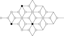
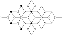
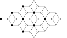
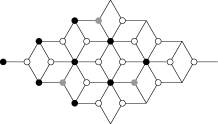
Figure 9: Ground state configurations of the charges (i.e. at $t=0$) for filling $1/9,2/9,1/3,4/9$. The different ground states occurs on increasing the value of the external charge $n_{0}$ The black circles denote those sites that are occupied by one Cooper pair. The ground state configurations are responsible for the behaviour of the phase correlator and hence of the lobe-like structure, Fig.10, of the phase diagram.

Figure 10: Lobe structures at different values of the capacity, i.e. electrostatic range (respectively $C=0,10^{-2},10^{-1},1$). The dashed lines point out the discrete filling of the ground state. Pictures on the right are magnifications of the highlighted areas in the left ones.

The phase diagram in the presence of charge frustration has a lobe structure fisher89 in which, progressively on increasing the external charge, the filling factor increases as well. In the case of finite range charging interaction also Mott lobes with fractional fillings appear bruder93 . An analytical determination of the ground state of the charging Hamiltonian for generic values of the external charge is not available. We considered rational fillings of the whole lattice as made up of periodic repetitions of a partially filled super-cell of size comparable with the range of the interaction $\mathcal{U}_{i,j}$ and then constructed a Wigner crystal for the Cooper pairs with this periodicity. For $C/C_{0}\leq 1$ a $3\times 3$ super-cell turns out to be sufficient. Given a certain rational filling $p/q$, the corresponding charging energy is given by

$$E_{\{n_{i}\}}(\frac{p}{q},n_{0})=3N\,\frac{e^{2}}{C_{0}}\,\left(n_{0}^{2}-2\frac{p}{q}n_{0}+\frac{C_{0}}{N}\,\sum_{i,j}n_{i}\mathcal{C}^{-1}_{i,j}n_{j}\right)$$

where $N$ is the number of cells in the system and $\{n_{i}\}$ is the particular realization of the filling.

This defines a set of parabolas which allow to determine the sequence of ground states. The variation of the ground state configurations as a function of gate charge gives to the phase boundary a characteristic structure made of lobes, as shown in Fig. 10. The longer is this range of the electrostatic interaction the richer is the lobe structure.

As can be seen in Fig. 10 when the interaction is purely on-site there is only one lobe that closes at half filling when the degeneracy between the empty ground state and the extra-charged one leads to superconductivity for arbitrarily small $t$. As soon as the range becomes finite, other fillings come into play. An interesting feature typical of the $\mathcal{T}_{3}$ lattice is that at $n_{0}=1/2$ the half filled state is not the ground state (see Fig. 10).

Finally, we recall that the presence of the offset breaks the particle-hole symmetry and thus the universality class of the phase transition change fisher89 . This can be seen from the expansion at small $\omega$ of the correlator (Eq. 13) that enters the quadratic term of the Wilson-Ginzburg-Landau functional. With $n_{0}$ also terms linear in $\omega$ enter the expansion and the dynamical exponent $z$ changes from $1$ to $2$.

IV.3 Magnetic frustration and Aharonov-Bohm insulating phase

The outgrowing interest in $\mathcal{T}_{3}$ lattices is especially due to their behaviour in the presence of an externally applied magnetic field. The presence of a magnetic field defines a new length scale, the magnetic length. The competition between this length and the lattice periodicity generates interesting phenomena such as the rising of a fractal spectrum à la Hofstadter. In $\mathcal{T}_{3}$ lattices perhaps the most striking feature is the complete localization in a fully frustrating field ($f=1/2$). This is due to destructive interference along all paths that particles could walk on, when the phase shift around a rhombic plaquette is $\pi$ (see Fig. 11). Is there any signature of this localization (originally predicted for tight-binding models) in the quantum phases transition between the Mott and the superconducting phases? This is what we want to investigate in this section.

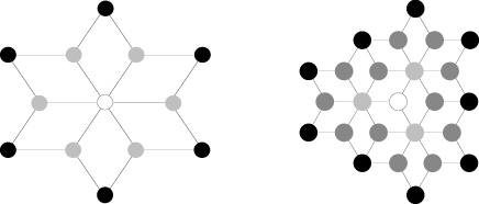
Figure 11: Aharonov-Bohm cages. Particles that starts on white sites can’t go further than black sites, due to destructive interference. In fact, $f=1/2$ means $\pi$ phase shift around a plaquette. In square lattices this could not happen because of the escape opportunity given by straight lines.

In order to determine the phase boundary at $T=0$ we can follow either the mean field approach of Sec. III.1 or the perturbative theory presented in Sec. III.3. We remind that while the first approach signals the disappearance of the superfluid phase, the perturbation expansion indicates where the Mott phase ends. The results of both approaches are shown in Fig. 12. Commensurate effects are visible in the phase boundary of Fig. 12 at rational fractions $f=p/q$ of the frustration. The results presented are quite generic. We decided to show, as a representative example, the results for a JJ array with capacitance ratio $C/C_{0}=1$ and an optical lattice with $U_{r}-U_{h}=0.5U_{h}$. The peak at $f=1/2$, characteristic of the $\mathcal{T}_{3}$ lattice is due to the presence of the Aharonov-Bohm cages.

Although there is a difference between the mean-field and the strong coupling calculation, they both confirm the same behaviour. A very interesting point however emerges at half-filling. It is worth to stress again that while the mean-field shows the disappearance of the superconducting phase, the strong coupling expansion indicates where the Mott gap vanishes and hence charges can condense. The vanishing of the gap can be associated to boson condensation only if bosons are delocalized. This is the case for the whole range of frustrations except at $f=1/2$. In the fully frustrated case the excitation gap vanishes but the excited state (the extra boson on a hub) still remains localized due to the existence of the Aharonov-Bohm cages. This may lead to the conclusion that at fully frustration there is an intermediate phase where the system is compressible (the Mott gap has been reduced to zero) with zero superfluid density (the bosons are localized in the Aharonov-Bohm cages).

At this level of approximation there is no way to explore further this scenario. In order to assess the existence of the intermediate phase a more accurate location of the phase boundaries is necessary. We will discuss the possible existence of the Aharonov-Bohm insulator by means of Monte Carlo simulations in the next section.

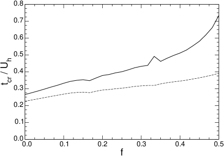
Figure 12: Phase boundary in presence of a magnetic field in $\mathcal{T}_{3}$: straight line is the perturbative result, mean field is dashed. Upper: JJAs with $C/C_{0}=1$; lower: optical lattices with $U_{r}-U_{h}=0.5U_{h}$. Note the highly pronounced peak at $f=1/2$ in contrast to the square lattice case.

IV.4 MonteCarlo methods

The simulations are performed on an effective classical model obtained after mapping the model of Eq.(3) onto a $(2+1)$ XY model. Our main interest in performing the Monte Carlo simulation is to look for signatures of the Aharonov-Bohm insulator. As its existence should not depend on the exact form of the repulsion $\mathcal{U}_{i,j}$ we chose the simplest possible case in which the repulsion is on-site and $U_{h}\sim U_{r}$. The details of the mapping are described in Refs. jacobs88, ; wallin94, and are briefly reviewed in Sec. A. The effective action $\mathcal{S}$ (at zero charge frustration) describing the equivalent classical model is

$$\mathcal{S} = K\,\sum_{\begin{array}[]{c}\langle i,\,j\rangle,k\end{array}}\left[1-\cos\left(\varphi_{i,k}-\varphi_{j,k}-A_{i,j}\right)\right]$$ (28)

$$+ K\,\sum_{\begin{array}[]{c}i,\langle k,\,k^{\prime}\rangle\end{array}}\left(1-\cos\left(\varphi_{i,k}-\varphi_{i,k^{\prime}}\right)\right)\;.$$ (30)

where the coupling $K$ is $\sqrt{t/U}$. The index $k$ labels the extra (imaginary time) direction which takes into account the quantum fluctuations. The simulations where performed on $L\times L\times L_{\tau}$ lattice with periodic boundary conditions. The two correlation lengths (along the space and time directions) are related by the dynamical exponent z through the relation $\xi_{\tau}\sim\xi^{z}$. For zero magnetic frustration, because of the particle-hole symmetry (we consider only the case $n_{0}=0$) holds $z=1$. As we will see this seems not to be the case at fully frustration because of the presence of the Aharonov-Bohm cages.

The evaluation of the various quantities have been obtained averaging up to $3\times 10^{5}$ Monte Carlo configurations for each one of the $10^{2}$ initial conditions, by using a standard Metropolis algorithm. Typically the first $10^{5}$ were used for thermalization. The largest lattice studied was $24\times 16\times 24$ at fully frustration and $48\times 48\times 48$ at $f=0$. This difference is due to the much larger statistics which is needed to obtain sufficiently reliable data. While in the unfrustrated case we took a cube of length $L$ in the fully frustrated case it turned out to be more convenient to consider (but will discuss other lattice shapes) an aspect ratio of $2/3$. With this choice the equilibration was simpler probably due to a different proliferation of domain wallskorshunov02 ; cataudella03 .

In order to characterize the phase diagram we studied the superfluid stiffness and the compressibility of the Bose-Hubbard model on a $\mathcal{T}_{3}$ lattice. The compressibility, $\kappa$, is defined by $\kappa=\partial^{2}\mathcal{F}/\partial V_{0}^{2}$ where $\mathcal{F}$ is the free energy of the system and $V_{0}$ the chemical potential for the bosons. By employing the Josephson relation in imaginary time, see Ref.wallin94 , the compressibility can be expressed as the response of the system to a twist in imaginary time, $\varphi_{i,k}\rightarrow\varphi_{i,k}+\theta_{\tau}\,k$, i.e.

$$\kappa=\left.\frac{\partial^{2}\mathcal{F}(\theta_{\tau})}{\partial{\theta^{2}_{\tau}}}\right|_{\theta_{\tau}=0}\ \;.$$ (31)

The superfluid stiffness is associated to the free energy cost to impose a phase twist in a direction $\mathbf{e}$, i.e. $\varphi_{i}\rightarrow\varphi_{i}+\theta_{\mathbf{e}}\,\mathbf{e}\cdot\mathbf{r}_{i}$, through the array

$$\gamma=\left.\frac{\partial^{2}\mathcal{F}(\theta_{\mathbf{e}})}{\partial{\theta^{2}_{\mathbf{e}}}}\right|_{\theta_{\mathbf{e}}=0}\;\;.$$ (32)

IV.4.1 f=0

In the case of unfrustrated system we expect that the transition belongs to the $3D-XY$ universality class. Close to the quantum critical point $\kappa\sim\xi^{-1}$, the corresponding finite size scaling expression for the compressibility reads

$$\kappa=L^{-(d-z)}\,\widetilde{\kappa}\left(L^{1/\nu}\,\frac{K-K_{c}}{K_{c}},\,\frac{L_{\tau}}{L^{z}}\right)$$ (33)

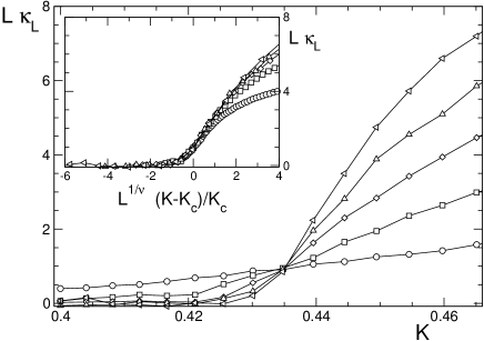
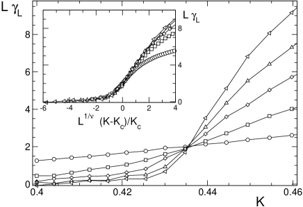
Figure 13: $f=0$: a)Scaling (main) and data collapse (inset) of the compressibility for the unfrustrated case. b)The same as in a) for the superfluid stiffness. All the systems have aspect ratio $L_{\tau}=L_{y}=L_{x}$ with $L_{\tau}=6$ (circles), 12 (squares), 18 (diamonds), 24 (triangles up), 30 (triangles down)

An analogous expression holds for the finite size-scaling behaviour of the stiffness

$$\gamma=L^{-(d+z-2)}\,\widetilde{\gamma}\left(L^{1/\nu}\,\frac{K-K_{c}}{K_{c}},\,\frac{L_{\tau}}{L^{z}}\right)$$ (34)

The expected exponent is $\nu=2/3$ as it is known from the properties of the three-dimensional $XY$ model.

The results of the simulations for the compressibility and for the stiffness are reported in Fig.13. Finite size scaling shows that the SI transition occurs at

$$K_{c}=0.435\pm 0.0025\;\;.$$ (35)

As expected the unfrustrated case follows remarkably well the standard picture of the Superfluid-Mott Insulator quantum phase transition. In the absence of the magnetic field the system defined by Eq.(28) is isotropic in space-time and therefore the stiffness and the compressibility have the same scaling and critical point.

IV.4.2 $f=\frac{1}{2}$

The situation changes dramatically in the fully frustrated system. In this case an anisotropy in space and time directions arises because of the presence of the applied magnetic field which frustrates the bonds in the space directions (see the r.h.s of Eq.(28)). This field induced anisotropy is responsible for the different behaviour of the system to a twist in the time (compressibility) or space (stiffness) components.

As already observed in the classical case cataudella03 , the Monte Carlo dynamics of frustrated $\mathcal{T}_{3}$ systems becomes very slow. This seems to be associated to the presence of zero-energy domain walls first discussed by Korshunov in Ref. korshunov02, . This issue is particulary delicate for the superfluid stiffness. In this case the longest simulations had to be performed. Moreover in order to alleviate this problem we always started the run deep in the superfluid state and progressively increased the value of the Hubbard repulsion $U$. Also the choice of the lattice dimensions turned out to be important. We made the simulations on $12\times 8\times 12$, $18\times 12\times 18$, and $24\times 16\times 24$ systems and found out that by choosing this aspect ratio along the $x$ and $y$ directions thermalization was considerably improved.

The results of the simulations are reported in Fig.14 for the compressibility and for the stiffness. As it appears from the raw data of the figure it seems that the points at which the compressibility and the stiffness go to zero are different. An appropriate way to extract the critical point(s) should be by means of finite size scaling.

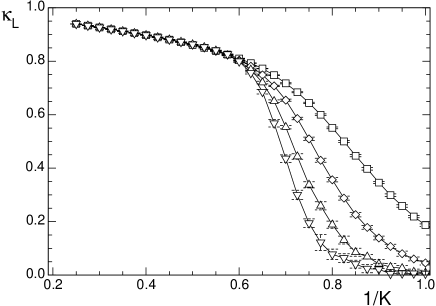
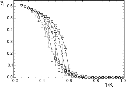
Figure 14: $f=1/2$:Compressibility (upper panel) and stiffness (lower panel) assuming the aspect ratio $L\times L\times 2L/3$. Different symbols corresponds to $L=$ 12 (circles), 18 (squares), 24 (triangles up), and 30 (triangles down).

As a first attempt we assumed that the transition is in the same universality class as for the unfrustrated case and we scaled the data as in Fig.13. Although the scaling hinted at the existence of two different critical points for the Mott to Aharonov-Bohm insulator and for the Aharonov-Bohm insulator to superfluid transitions respectively, the quality of the scaling points was poor. In our opinion this observation may suggest that the scaling exponents for the fully frustrated case are different as the one for the direct Mott Insulator to Superfluid phase transition at $f\neq 1/2$. In order to extract more tight bounds on the existence of this phase we analyzed the size dependence of the observables without any explicit hypothesis on the scaling exponent (which we actually do not know). The results are presented in Fig.15.

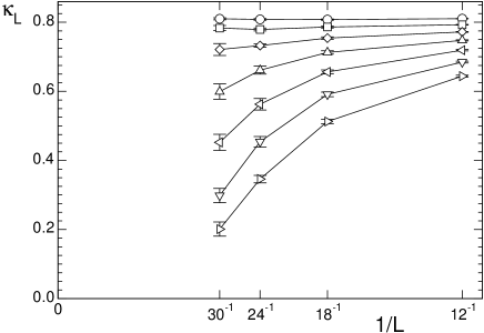
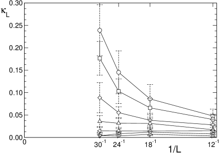
Figure 15: $f=1/2$: Compressibility (upper panel) and the stiffness (lower panel) as a function of the $L_{t}$ size of the system for different values of $K$. Data corresponds to $1/K=0.6$(circles), $0.625$(squares), $0.65$(diamonds), $0.675$(triangles up), $0.7$(tr. left), $0.725$(tr. down), $0.75$(tr. right).

.

The data of Fig.15 seem to indicate that there is a window

$$0.65\leq K^{-1}\leq 0.7$$

where the system is compressible but not superfluid! This new phase, the Aharonov-Bohm insulator, is the result of the subtle interplay of the $\mathcal{T}_{3}$ lattice structure and the frustration induced by the external magnetic field. Our simulations cannot firmly determine the existence of two separate critical points since we were not able to improve their accuracy and study larger lattices. However we think that, by combining both the analytical results and the Monte Carlo data we have a possible scenario for the phase diagram of the frustrated BH model on a $\mathcal{T}_{3}$ lattice.

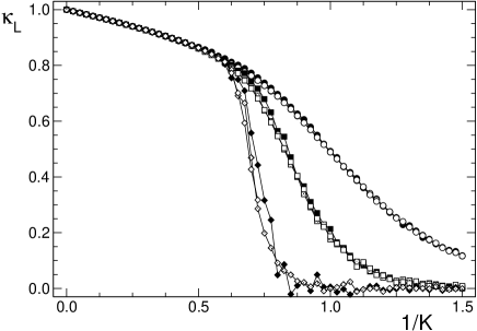
Figure 16: Compressibility as a function of $K=\sqrt{t/U}$ for different values of the system sizes. Different symbols corresponds to different lengths $L_{\tau}$ in the time dimension: 6 (circles), 12 (squares), and 30 (diamonds). Different fillings are different spatial sizes $L_{x}\times L_{y}$: $6\times 4$ (black), $12\times 8$ (gray), and $18\times 12$ (white). The compressibility depends strongly on $L_{\tau}$ but very weakly on $L_{x}\times L_{y}$.

Further evidence of the existence of the AB cages can be obtained by analyzing the anisotropy in space and time directions of the phase correlations. For this purpose we considered the compressibility as a function of $L$ and $L_{\tau}$ separately. The idea is that because of the AB cages the correlations are short-ranged in the space directions (bosons are localized) while there are longer ranged correlations in the time direction. Indeed the dependence of the compressibility on the system dimensions is strong when one changes $L_{\tau}$ while it is rather weak when the space dimensions are varied as shown in Fig.16. This hints at the fact that the Aharonov-Bohm phase is a phase in which the gap has been suppressed (correlation in the time dimension) but where the bosons are localized (short-range correlations in space).

The Monte Carlo simulations just discussed provide evidence for the existence of a new phase between the Mott insulator and superfluid. Due to the finite size of the system considered and to the (present) lack of a scaling theory of the two transitions, we cannot rule out other possible interpretations of the observed behaviour of the Monte Carlo data. A possible scenario which is compatible with the simulations (but not with the result of the perturbation expansion footnote3 ) is that a single thermodynamic transition is present in the $2+1$ dimensional system but the phase coherence is established in a two step process. First the system becomes (quasi) ordered along the time direction, then, upon increasing the hopping the residual interaction between these “quasi-one-dimensional” coherent tubes go into a three-dimensional coherent state driven by the residual coupling between the tubes. In more physical terms the “tubes” represent the boson localized in the AB cages and the residual hopping is responsible for the transition to the superfluid state. This means that the intermediate state that we observe is due to a one- to three-dimensional crossover that takes place at intermediate couplings.

V Conclusions

In this work we exploited several methods, both analytic and numerical, in order to determine the phase diagram of a Bose-Hubbard model on a $\mathcal{T}_{3}$ lattice. Differently from previous studies on $\mathcal{T}_{3}$ networks we analyzed the situation where the repulsion between bosons (or Cooper pairs for Josephson arrays) becomes comparable with the tunnelling amplitude (Josephson coupling in JJAs) leading to a quantum phase transition in the phase diagram. Up to now the attention on experimental implementations has been confined to Josephson networks. As discussed in Sec. II.2, the $\mathcal{T}_{3}$ lattice can also be realized in optical lattices. The possibility to experimentally study frustrated $\mathcal{T}_{3}$ optical lattices open the very interesting possibility to observe subtle interference phenomena associated to Aharonov-Bohm cages also with cold atoms. Having in mind both the realization in Josephson and optical arrays, we studied a variety of different situations determined by the range of the boson repulsion including both electric and magnetic frustration. Although in the whole paper we concentrated on the $T=0$ case, in this discussion we will also comment on the finite temperature phase diagram.

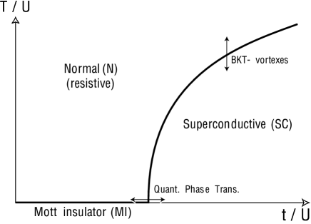
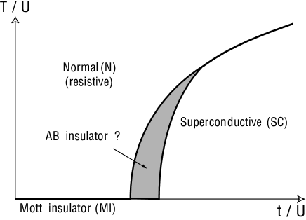
Figure 17: A possible phase diagram of an array with $\mathcal{T}_{3}$ lattice. In the unfrustrated case (upper panel) we sketch the standard phase diagram which leads at $T=0$ to the SI transition. On the lower panel we present a possible scenario that emerges from our work. An new phase appears separating the normal from the superfluid phases.

The peculiarity of the lattice symmetry already emerges for the unfrustrated case. The superfluid phase is not uniform but it has a modulation related to the presence of hubs and rims with different coordination number. As a function of the chemical potential (gate charge) the transition has a quite rich structure due to the different boson super-lattices which appear as the ground state.

As a function of the magnetic field the SI transition has the characteristic butterfly form. In the fully frustrated case, however, the change is radical and we find indications that the presence of the Aharonov-Bohm cages can lead to the appearance of a new phase, the Aharonov-Bohm insulator. This phase should be characterized by a finite compressibility and zero superfluid stiffness. A sketch of the phase diagram is shown in Fig.17. With the help of Monte Carlo simulations we were able to bound the range of existence of the new phase. Unfortunately we have to admit that our results are not conclusive and, as discussed in the previous section, an alternative scenario is also possible. Nevertheless, we think that the existence of an intermediate phase is a very appealing possibility worth to being further investigated.

How is it possible to experimentally detect such a phase? In Josephson arrays, where one typically does transport measurement, the AB-insulator should be detected by looking at the temperature dependence of the linear resistance. On approaching the zero temperature limit, the resistance should grow as $T^{\delta}$ differently from the Mott insulating phase where it has an exponential activated behaviour. In optical lattices the different phases can be detected by looking at the different interference pattern (in the momentum density or in the fluctuations altman04 ). A detailed analysis of the experimental probe will be performed in a subsequent publication.

There are several issues that remain to be investigated. It would be important, for example, to see how the phase diagram of the frustrated system (and in particular the Aharonov-Bohm phase) is modified by a finite range of $\mathcal{U}_{i,j}$ and/or the presence of a finite chemical potential. An interesting possibility left untouched by this work is to study the fully frustrated array at $n_{0}=1/2$. In this case (for on-site interaction) the superfluid phase extends down to vanishing small hopping. In this case a more extended AB insulating phase could be more favoured, and thus more clearly visible.

Appendix A (2+1)D XY mapping

We give here some of the technical details of the mapping from the QPM to a $(2+1)D-XY$ model. The latter one is particularly easy to be simulated numerically: the state of the system and the effective action are both expressed in terms of phases on a $3D$ lattice. Being $n$ and $\varphi$ canonically conjugated, it is possible to represent $n$ as $-\imath\frac{\partial\,}{\partial\varphi}$ and get the so-called quantum rotor Hamiltonian. For the sake of simplicity we consider a diagonal capacitance matrix.

$$\mathcal{H} = \mathcal{H}_{t}+\mathcal{H}_{U}$$

$$\mathcal{H}_{U} = -\frac{U}{2}\sum_{\mathbf{r}}\frac{\partial^{2}\,}{\partial\varphi_{\mathbf{r}}^{2}}$$

$$\mathcal{H}_{t} = -t\sum_{\langle i,j\rangle}\cos(\varphi_{i}-\varphi_{j}-A_{i,j})$$ (36)

The partition function can be rewritten in a more convenient way using the Trotter approximation:

$$\mathcal{Z} = \mbox{Tr}\left\{(e^{-\frac{\beta}{L_{\tau}}(\mathcal{H}_{t}+\mathcal{H}_{U})})^{L_{\tau}}\right\}$$ (37)

$$= \lim_{L_{\tau}\rightarrow\infty}\mbox{Tr}\left\{(e^{-\Delta\tau\mathcal{H}_{U}}e^{-\Delta\tau\mathcal{H}_{t}}+o(\Delta\tau^{2}))^{L_{\tau}}\right\}$$

where $\hbar\tau$ is imaginary time and $\Delta\tau=\beta/L_{\tau}$ is the width of a time slice. The limit $\Delta\tau\rightarrow 0$ must be taken to recover the underlying quantum problem.

Introducing complete sets of states $|\overrightarrow{\varphi(\tau_{k})}\rangle$ with periodic boundary conditions on times ($\tau_{0}=0\ \equiv\ \tau_{L_{\tau}}=\beta$) the trace can be written as

$$\mathcal{Z}=\int\mathcal{D}\varphi\prod_{k=0}^{L_{\tau}}\langle\overrightarrow{\varphi(\tau_{k+1})}|e^{-\Delta\tau\,\mathcal{H}_{U}}e^{-\Delta\tau\,\mathcal{H}_{t}}|\overrightarrow{\varphi(\tau_{k})}\rangle$$ (38)

Since the states $|\overrightarrow{\varphi(\tau_{k})}\rangle$ are eigenstates of $\mathcal{H}_{t}$, the calculation is reduced to the evaluation of the matrix elements

$$\langle\overrightarrow{\varphi(\tau_{k+1})}|e^{-\Delta\tau\,\mathcal{T}}|\overrightarrow{\varphi(\tau_{k})}\rangle.$$ (39)

the matrix elements can be furtherly simplified going back to the charge representation (or angular momentum, since $n$ is the generator of $U(1)$ for the $XY$ spin of a site):

$$\sum_{\overrightarrow{J^{\tau}}}\prod_{i}e^{-\frac{U\,\Delta\tau}{2}[J^{\tau}_{i}]^{2}}e^{\imath\,J^{\tau}_{i}\,[\varphi_{i}(\tau_{k})-\varphi_{i}(\tau_{k+1})]}.$$ (40)

Using the Poisson summation formula, the sum over angular momentum configurations becomes a periodic sequence of narrow gaussians around multiples of $2\pi$

$$\prod_{i}\,\sum_{m=-\infty}^{+\infty}\sqrt{\frac{2\pi}{U\,\Delta\tau}}\,e^{-\frac{1}{2\,\Delta\tau\,U}[\varphi_{i}(\tau_{k})-\varphi_{i}(\tau_{k+1})-2\pi m]^{2}}$$ (41)

that is the Villain approximation to

$$\mathcal{T}_{k}\approx\prod_{i}\,e^{-\frac{1}{U\,\Delta\tau}\cos[\varphi_{i}(\tau_{k})-\varphi_{i}(\tau_{k+1})]}$$ (42)

with dropped irrelevant prefactors.

What we get by means of this procedure is a mapping of the QPM into a anisotropic classical $(2+1)DXY$ model, with effective action $\mathcal{S}$

$$\mathcal{S} = K_{sp}\ \sum_{\langle i,\,j\rangle,k}\left[1-\cos\left(\varphi_{i,k}-\varphi_{j,k}-A_{i,\,j}\right)\right]$$ (44)

$$+ K_{\tau}\ \sum_{i,\langle k,\,k^{\prime}\rangle}\left[1-\cos\left(\varphi_{i,k}-\varphi_{i,k^{\prime}}\right)\right]$$

$$K_{sp}=t\,\Delta\tau\hskip 28.45274ptK_{\tau}=\frac{1}{U\,\Delta\tau}$$

where we used a symmetric notation for space and time lattice sites. Since critical properties are not expected to depend on the asymmetry of such model, and since for $\Delta\tau\longrightarrow 0$ we have $K_{sp}\longrightarrow 0,\ \ K_{\tau}\longrightarrow\infty\ \ \mbox{with}\ K_{sp}\,K_{\tau}=\mbox{const.}$, one can fix $\Delta\tau=1/\sqrt{tU}$. It then follows that the coupling in the space and time directions are equal $K_{sp}=K_{\tau}=K$. The isotropic model, Eq.(28) is the one which is used in in the Monte Carlo simulations.

References

- (1) M.P.A. Fisher, P. B. Weichman, G. Grinstein, and D. S. Fisher, Phys. Rev. B 40, 546 (1989).
- (2) S.L. Sondhi, S.M. Girvin, J.P. Carini, D. Shahar, Rev. Mod. Phys. 69, 315 (1997).
- (3) R. Fazio and H.S.J. van der Zant, Phys. Rep. 355, 235 (2001).
- (4) D. Jaksch, C. Bruder, J.I. Cirac, C.W. Gardiner, P.Zoller, Phys. Rev. Lett. 82, 3108 (1998).
- (5) M. Greiner, O. Mandel, T. Esslinger, T.W. H nsch, I. Bloch, Nature 415, 39 (2002).
- (6) J. Villain, J. Phys. C 10, 1717 (1977); W.Y. Shih and D. Stroud, Phys. Rev. B 30, 6774 (1984); D.H. Lee, J. D. Joannopoulos, J. W. Negele, and D.P. Landau, Phys. Rev. Lett. 52, 433 (1984); H. Kawamura, J. Phys. Soc. Jpn. 53, 2452 (1984); M.Y. Choi and S. Doniach, Phys.Rev. B 31, 4516 (1985); T.C. Halsey, Phys. Rev. B 31, 5728 (1985); S. E. Korshunov, J. Phys. C 19, 5927 (1986);
- (7) D. Jaksch and P. Zoller, New J. Phys. 5, 56 (2003).
- (8) A.S. Sørensen, E. Demler, and M.D. Lukin, Phys. Rev. Lett. 94, 086803 (2005).
- (9) M. Polini, R. Fazio, A.H. MacDonald, and M.P. Tosi, Phys. Rev. Lett. 94, 010401 (2005).
- (10) K. Osterloh, M. Baig, L. Santos, P. Zoller, M. Lewenstein, Phys. Rev. Lett. 95, 010403 (2005).
- (11) B. Sutherland, Phys. Rev. B 34, 5208 (1986).
- (12) J. Vidal, R. Mosseri and B. Douçot, Phys. Rev. Lett. 81, 5888 (1998).
- (13) C. Abilio, P. Butaud, Th. Fournier, B. Pannetier, J. Vidal, S. Tedesco and B. Dalzotto, Phys. Rev. Lett. 83, 5102 (1999).
- (14) E. Serret, P. Butaud, B. Pannetier, Europhys. Lett. 59, 225 (2003).
- (15) C. Naud, G. Faini, and D. Mailly Phys. Rev. Lett. 86, 5104 (2001).
- (16) S.E. Korshunov, Phys. Rev. B 65, 054416 (2002).
- (17) V. Cataudella and R. Fazio, Europhys. Lett. 61, 341 (2003).
- (18) S.E. Korshunov and B. Douçot, cond-mat/0310536.
- (19) B. Douçot and J. Vidal, Phys. Rev. Lett. 88, 227005 (2002).
- (20) I.V. Protopopov and M.V. Feigel’man, Phys. Rev. B 70, 184519 (2004).
- (21) D. Bercioux, M. Governale, V. Cataudella, and V. Marigliano Ramaglia, Phys. Rev. Lett. 93, 56802 (2004); cond-mat/0502455.
- (22) C. Bruder, R. Fazio, and G. Schön, Phys. Rev. B 47, 342 (1993).
- (23) R.F. Voss and R.A. Webb, Phys. Rev. B 25, 3446 (1982); R.A. Webb, R.F. Voss, G. Grinstein and P.M. Horn, Phys. Rev. Lett. 51, 690 (1983).
- (24) J.E. Mooij and G. Schön (Eds.), Coherence in Superconducting Networks, Physica B 152, 1-302 (1988); H.A. Cerdeira and S.R. Shenoy (Eds.), Josephson junctions arrays, Physica B 222, 253-406 (1996).
- (25) J.Resnick, J. Garland, J. Boyd, S. Shoemaker and R. Newrock, Phys. Rev. Lett. 47, 1542 (1981); P. Martinoli, P. Lerch, C. Leemann and H. Beck, J. Appl. Phys. 26, 1999 (1987).
-
(26)
V. Berezinski, Zh. Exsp. Teor. Fiz. 59, 907
(1970);
J.M. Kosterlitz, D.J. Thouless, J. Phys. C 6, 1181 (1973). - (27) In this paper we consider the case finite range interaction, for the case of see J. E. Mooij, B. J. van Wees, L. J. Geerligs, M. Peters, R. Fazio, and G. Schön, Phys. Rev. Lett. 65, 645 (1990).
- (28) D.S. Rokhsar and G.B. Kotliar, Phys. Rev. B 44, 10328 (1991).
- (29) J. K. Freericks and H. Monien, Phys. Rev. B 53, 2691 (1996).
- (30) M. Niemeyer, J. K. Freericks, and H. Monien Phys. Rev. B 60, 2357 (1999).
- (31) B.J. Kim, G.S. Jeon, M.S. Choi, M.Y. Choi, Phys. Rev. B 58, 14524 (1998).
- (32) L. Jacobs, J. V. Jos , M. A. Novotny, and A. M. Goldman Phys. Rev. B 38, 4562 (1988).
- (33) M. Wallin, E.S. Sørensen, S. M. Girvin, and A. P. Young, Phys. Rev. B 49, 12115 (1994).
- (34) In the perturbation expansion, the eigenfunction corresponding to the excited state is localized in space. Therefore one should not expect any condensation to a superfluid state.
- (35) E. Altman, E. Demler, and M.D. Lukin, A 70, 013603 (2004).