’Electron’ and ’photon’ emerging from supersymmetric neutral particles: A possible realization in ultracold Bose-Fermi atom mixture

Abstract

We show that the ’electron’ and ’photon’ can emerge from a supersymmetric Hubbard model which is a non-relativistic theory of the neutral particles. The Higgs boson and ’photon’ may not appear in the same phase of the phase diagram. In a Mott insulator phase of the boson, the ’electron’ and ’photon’ are stablized by an induced Coulomb interaction between ’electrons’. This emergent mechanism may be ’realized’ in an ultracold Bose-Fermi atom mixture except the long range Coulomb interaction is repalced by a nearest neighbor one. We suggest to create ’external electric field’ so that the ’electron’ excitation can be observed by measuring the linear density-density response of the ’electron’ gas to the ’external field’ in the time flying experiment of the mixture. The Fermi surface of the ’electron’ gas may also be expected to be observed in the time flying.

What roles did the mysterious Higgs boson play except providing a mass to the intermediate bosons in the weak-electrodynamics? Where did the electron and photon come from wen ? In this Letter, we suggest that it was a neutral world in high temperature and the electrons and photons emerged when the temperature was lower than certain critical temperature. The Higgs boson fluctuation plays an important role in the appearance of the finite gauge coupling constant. We show that this emergence can be ’realized’ by the elementary excitations in the ultracold Bose-Fermi atom mixture in optical lattices except the Coulomb interaction between ’electrons’ is replaced by a nearest neighbor one.

We start from a three-dimensional spinless supersymmetric(SUSY) Hubbard model, which was called ’ultracold superstring’ in one-dimensional lattice stoof . The microscopic description of the model parameters for an ultracold atom mixture has been proposed aie . The constitution particles in this model are neutral spinless bosons ($a_{i}$) and fermions ($f_{i}$) with $i$ the lattice site index. In high temperatures, there are only excitations of these constitution particles. We call this a confinement phase. After the SUSY is broken, the system undergoes a phase transition, in certain critical temperature, to a uniform mean field (UMF) state in which a finite coupling gauge field and a ’charged’ fermion emerge if the fermion occupation is nearly half filling. We call these emergent objects ’photon’ and ’electron’, respectively. At the exact half filling, this UMF state turns to a long range ordered state, the checkerboard crystal comp . However, this UMF state can only be stable if the lattice filling of the constitution bosons is integer and has a Mott insulator (MI) ground state. For a special space structure, the ’electron’ interaction is pure Coulomb.

Experimentally, the Bose-Fermi atom mixture in optical lattices has been realized for ⁸⁷Rb-⁴⁰K rbk , and ²³Na-⁶Li nali . We suggest an experiment to create an ’external field’ by changing the depth of the fermion’s optical potential. The response function of the mixture to the external field may be measured by the density distribution in a time flying of the cold atom cloud. The behavior of the response functions may be used to identify the fermionic elementary excitations in a set of given parameters, either the constitution one or ’electronic’. On the other hand, we expect the ’electron’ Fermi surface can be observed by the time flying, which has been used to observe the Fermi surface of the pure cold Fermi atoms kms .

The Bose-Fermi mixture Hubbard Hamiltonian we are interested in reads

$$H = -\sum_{i\neq j}(t_{B,ij}a^{\dagger}_{i}a_{j}+t_{F,ij}f^{\dagger}_{i}f_{j})-\sum_{i}(\mu_{B}n^{a}_{i}+\mu_{F}n^{f}_{i})$$ (1)

$$+ \frac{U_{BB}}{2}\sum_{i}n^{a}_{i}(n^{a}_{i}-1)+U_{BF}\sum_{i}n^{a}_{i}n^{f}_{i},$$

where the lattice spacing is set to unit. $n^{a}_{i}=a^{\dagger}_{i}a_{i}$ and $n^{f}_{i}=f^{\dagger}_{i}f_{i}$. $t_{B,ij}$ and $t_{F,ij}$ are the hopping amplitudes of the boson and fermion between a pair of sites. $\mu_{B}$ and $\mu_{F}$ are chemical potentials. And $U_{BB}$ and $U_{BF}$ are the on-site interactions between bosons, and between boson and fermion, both of which may be repulsive or attractive. The microscopic calculations of these model parameters in terms of the cold atom mixture may be found, e.g, in Ref. aie . If $t_{B,ij}=t_{F,ij}=t_{ij}$, $\mu_{B}=\mu_{F}=\mu$ and $U_{BB}=U_{BF}=U$, the model is SUSY under transformations $\delta a_{i}=i\theta f_{i},~{}~{}~{}\delta f_{i}=i\theta a_{i}$ where $\theta$ is a Grassmann number.

To deduce the low energy theory in strong couplings , we will use the slave particle technique, which has been applied to the cold boson system d ; yu ; lu . In the slave particle language, the Hamiltonian reads $H=H_{2}+H_{4}$ where $H_{2}$ and $H_{4}$ are the two-operator and four-operator terms, respectively. Namely,

$$H_{2}=-\sum_{i}\sum_{\alpha}[\mu_{B}\alpha(n^{\alpha}_{c,i}+n^{\alpha}_{h,i})+\mu_{F}n^{\alpha}_{c,i}]$$ (2)

$$+\frac{U_{BB}}{2}\sum_{i}\sum_{\alpha}\alpha(\alpha-1)(n_{c,i}^{\alpha}+n_{h,i}^{\alpha})+U_{BF}\sum_{i}\sum_{\alpha}\alpha n_{c,i}^{\alpha},$$

and

$$H_{4} = -\sum_{ij}t_{F,ij}\sum_{\alpha,\beta}c^{\dagger}_{\alpha,i}h_{\alpha,i}h^{\dagger}_{\beta,j}c_{\beta,j}$$

$$- \sum_{ij}t_{B,ij}\sum_{\alpha,\beta}\sqrt{\alpha+1}\sqrt{\beta+1}$$

$$( h^{\dagger}_{\alpha+1,i}h_{\alpha,i}+c^{\dagger}_{\alpha+1,i}c_{\alpha,i})(h^{\dagger}_{\beta,j}h_{\beta+1,j}+c^{\dagger}_{\beta,j}c_{\beta+1,j}),$$

where $n^{\alpha}_{c,i}=c^{\dagger}_{\alpha,i}c_{\alpha,i}$ and $n^{\alpha}_{h,i}=h^{\dagger}_{\alpha,i}h_{\alpha,i}$. We explain briefly the deduction of this slave particle Hamiltonian. The state configurations at an arbitrary given site consists of $\{|\alpha,s\rangle~{}|~{}\alpha=0,1,2,...~{};~{}s=0,1\}$ where $\alpha$ and $s$ are the boson and fermion occupations, respectively. The Bose and Fermi creation operators can be expressed as $a^{\dagger}=\sum_{\alpha}\sqrt{\alpha+1}[|\alpha+1,0\rangle\langle\alpha,0|+|\alpha+1,1\rangle\langle\alpha,1|],f^{\dagger}=\sum_{\alpha}|\alpha,1\rangle\langle\alpha,0|$. The mapping to the slave particle reads $|\alpha,0\rangle\to h^{\dagger}_{\alpha},|\alpha,1\rangle\to c^{\dagger}_{\alpha}$ . We call $c_{\alpha}$ the composite fermion (CF) comp and $h_{\alpha}$ the slave boson. The normalized condition $\sum_{\alpha}(|\alpha,0\rangle\langle\alpha,0|+|\alpha,1\rangle\langle\alpha,1|)=1$ implies a constraint $\sum_{\alpha}(n^{\alpha}_{c}+n^{\alpha}_{h})=1$ at each site. The slave particles arise a $U(1)$ gauge symmetry $c_{\alpha,i}\to e^{i\varphi_{i}}c_{\alpha,i},h_{\alpha,i}\to e^{i\varphi_{i}}h_{\alpha,i}.$ The SUSY transformation is given by $\delta h_{\alpha,i}=i\theta\sqrt{\alpha}c_{\alpha-1,i},~{}~{}~{}\delta c_{\alpha,i}=i\theta\sqrt{\alpha+1}h_{\alpha+1,i}$. The global $U(1)$ symmetry $c_{\alpha,i}\to e^{i\alpha\varphi}c_{\alpha,i},h_{\alpha,i}\to e^{i\alpha\varphi}h_{\alpha,i}$ reflects the particle number conservation. Since the slave particle technique essentially works in the strong coupling region, we focus on $\bar{U}_{BB}=U_{BB}/|\varepsilon_{0}|\gg 1$ where $\varepsilon_{k}$ is the dispersion of the constitution boson. (Hereafter, a quantity $\bar{A}\equiv A/|\varepsilon_{0}|$.)

There are two types of four slave particle terms in $H_{4}$, the $t_{B}$ terms and $t_{F}$ terms. We first neglect the $t_{B}$ terms in the mean field level of the CF. To decouple the $t_{F}$ terms , we introduce Hubbard-Stratonovich fields $\hat{\eta}^{c,h}_{\alpha\beta,ij}$ and $\hat{\chi}^{c,h}_{\alpha\beta,ij}$. The partition function is given by $Z=\int D\hat{\chi}D\hat{\eta}D\bar{c}DcD\bar{h}DhD\lambda~{}e^{-S_{eff}}$ where the effective action reads

$$S_{eff}[\hat{\chi},\hat{\eta},c,h,\lambda]=\int_{0}^{1/T}d\tau\biggl{\{}\sum_{i}\sum_{\alpha}$$

$$\biggl{[}\bar{c}_{\alpha,i}(\partial_{\tau}-(\mu_{B}\alpha+\mu_{F})+\frac{U_{BB}}{2}\alpha(\alpha-1)$$

$$+U_{BF}\alpha-i\lambda_{i})c_{\alpha,i}+\bar{h}_{\alpha,i}(\partial_{\tau}-\alpha\mu_{B}$$

$$+\frac{U_{BB}}{2}\alpha(\alpha-1)-i\lambda_{i})h_{\alpha,i}\biggr{]}+\sum_{i}i\lambda_{i}$$

$$+\sum_{ij;\alpha,\beta}t_{F,ij}[\hat{\eta}^{h}_{\beta\alpha,ji}(\hat{\chi}^{c}_{\alpha\beta,ij}-\bar{c}_{\alpha,i}c_{\beta,j})-\hat{\chi}^{c}_{\alpha\beta,ij}\hat{\chi}^{h}_{\beta\alpha,ji}$$

$$+\hat{\eta}^{c}_{\alpha\beta,ij}(\hat{\chi}^{h}_{\beta\alpha,ji}-\bar{h}_{\beta,j}h_{\alpha,i})]+t_{B}~{}{\rm terms}\biggr{\}},$$ (4)

where $\lambda_{i}$ is the Lagrange multiplier for the constraint $\sum_{\alpha}(n^{\alpha}_{c,i}+n^{\alpha}_{h,i})=1$. Rewriting $\hat{\eta}^{c,h}_{\alpha\beta,ij}=\eta^{c,h}_{\alpha\beta,ij}e^{i{\cal A}_{ij}}$ and $\hat{\chi}^{c,h}_{\alpha\beta,ij}=\chi^{c,h}_{\alpha\beta,ij}e^{i{\cal A}_{ij}}$ and $\lambda_{i}=\lambda+{\cal A}_{0,i}$, ${\cal A}_{0i}$ and ${\cal A}_{ij}$ are $U(1)$ gauge field corresponding to the gauge symmetry. Fixing a gauge, $\hat{\eta}_{\alpha\beta,ij}^{h}\approx\eta^{h}_{\alpha,ij}\delta_{\alpha\beta}$, $\hat{\chi}_{\alpha\beta,ij}^{h}\approx\chi^{h}_{\alpha,ij}\delta_{\alpha\beta}$ and $\lambda_{i}\approx\lambda$ (which is a saddle point value of $\lambda_{i}$). This is corresponding to a mean field approximation. The effective mean field action is given by

$$S_{MF} = iN_{s}\beta\lambda+\int d\tau\biggl{\{}\sum_{\langle ij\rangle}(t_{F,ij}\sum_{\alpha}\chi^{c}_{\alpha,ij}\chi^{h}_{\alpha,ji})$$

$$+ \sum_{i\neq j}\sum_{\alpha}(\bar{c}_{\alpha,i}(D^{\alpha}_{c})^{-1}_{ij}c_{\alpha,j}+\bar{h}_{\alpha,i}(D^{\alpha}_{h})^{-1}_{ij}h_{\alpha,j})\biggr{\}}$$

where $(D^{\alpha}_{c})^{-1}_{ij}=(\partial_{\tau}-\mu^{\alpha}_{F})\delta_{ij}-t_{F}\sum_{\vec{\tau}}\chi^{h}_{\alpha,ji}\delta_{j,i+\vec{\tau}}$, $\mu^{\alpha}_{F}=\mu_{B}\alpha+\mu_{F}+\frac{U_{BB}}{2}\alpha(\alpha-1)+U_{BF}\alpha-i\lambda$ and $(D^{\alpha}_{h})^{-1}_{ij}=(\partial_{\tau}-\alpha\mu_{B}+\frac{U_{BB}}{2}\alpha(\alpha-1)-i\lambda))\delta_{ij}-t_{F}\sum_{\vec{\tau}}\chi^{c}_{\alpha,ji}\delta_{j,i+\vec{\tau}}$. ($\vec{\tau}$ is the unit vector of the lattice.) To simplify, we have assumed only the nearest neighbor hopping $t_{F}$ of the fermions is not zero.

The mean field equations are $\chi^{c}_{\alpha,ij}=\langle c^{\dagger}_{\alpha,i}c_{\alpha,j}\rangle=T\sum_{n}D^{\alpha}_{c,ij}(p_{n}),\chi^{h}_{\alpha,ij}=\langle h^{\dagger}_{\alpha,i}h_{\alpha,j}\rangle=T\sum_{n}D^{\alpha}_{h,ij}(\omega_{n})$ where $D^{\alpha}_{c,ij}(p_{n})=\int d\tau e^{ip_{n}\tau}D^{\alpha}_{c,ij}(\tau)$ and $D^{\alpha}_{h,ij}(\omega_{n})=\int d\tau e^{i\omega_{n}\tau}D^{\alpha}_{h,ij}(\tau)$ with $p_{n}$ and $\omega_{n}$ the Fermi and Bose frequencies. Solving the mean field equations near the critical point with $\chi^{\alpha}\approx 0$, one can obtain the critical temperature $T_{c}^{\alpha}$

$$T_{c}^{\alpha}=\sqrt{T^{\alpha}_{F}T^{\alpha}_{B}}$$ (6)

with $T^{\alpha}_{F,B}=t_{F}n^{\alpha}_{c,h}(1\mp n^{\alpha}_{c,h})$, $T^{\alpha}_{c}\chi^{c}_{\alpha,ij}=-T^{\alpha}_{F}\chi^{h}_{\alpha,ji}$ and $T^{\alpha}_{c}\chi^{h}_{\alpha,ij}=-T^{\alpha}_{B}\chi^{c}_{\alpha,ji}$ where $n_{h}^{\alpha}=1/[e^{\beta[-i\lambda-\alpha\mu_{B}+\alpha(\alpha-1)U_{BB}/2]}-1],n_{c}^{\alpha}=1/[e^{\beta[-i\lambda-(\alpha\mu_{B}+\mu_{F})+\alpha(\alpha-1)U_{BB}/2+\alpha U_{BF}]}+1]$. Below this temperature, the minimized free energy including variables $\chi$ is $F\propto-t_{F}\sum_{\alpha}(\tau^{\alpha})^{2}\frac{(S^{\alpha}_{2})^{2}}{S^{\alpha}_{4}}$ where $\tau^{\alpha}=\frac{T^{\alpha}_{c}-T}{T}$ and $S^{\alpha}_{2}$, $S^{\alpha}_{4}$ are the fractions of non-zero terms corresponding to the second order and four order of $|\chi^{\alpha}|$ il . The optimal $|\chi^{c}_{\alpha}|^{2}\propto\tau^{\alpha}S^{\alpha}_{2}/S^{\alpha}_{4}$.

Before going to a concrete mean field state, we first require the mixture is stable against the Bose-Fermi phase separation. For example, it was known that the mixture is stable in the MI phase if $4\pi t_{F}\sin(\pi n^{f})U_{BB}>U_{BF}^{2}$ aie . For the parameters in the SUSY model, this inequality is not satisfied. Thus, we assume the SUSY has been broken. In cold atom contents, the SUSY is broken by hands through changing the lattice potentials. If the real electron and photon are generated in the way described in this paper, the SUSY breaking might be related to the change of space-time structure in early universe, which has been beyond the present model.

We consider an integer boson filling $n^{a}=$1 for $\bar{U}_{BB}\gg 1$. In this region, since $n^{\alpha\neq 1}_{h}$ and $n^{\alpha\neq 1}_{c}$ are very small, there are no solutions of the mean field equations with $T^{\alpha\neq 1}_{c}\geq 0$ for the critical temperature equations. Thus, all slave bosons and CFs with $\alpha\neq 1$ are confined. Only $T^{1}_{c}>0$ can be found. Below $T_{c}^{1}$, the CF $c_{1}$ and the slave boson $h_{1}$ are deconfined in the mean field sense. We shall see the CF $c_{1}$ may be identified as the ’electron’ while $h_{1}$ as the Higgs boson. In the inset of Fig. 1, we plot $T_{c}^{1}$ for a set of given parameters. The curve $T_{p}(U_{BB})$ is corresponding to $\mu^{1}_{F}(T_{p})=0$, i.e., the effective chemical potential of $c_{1}$ vanishes. For the fermion half filling, $\mu_{F}^{1}(T=0)\to 0$. This means that the Fermi surface of CF $c_{1}$ shrinks and implies an insulating state, a checkerboard crystal as we shall see soon. Meanwhile, we also find $T_{c}^{1}=0$ for the half-filling of the fermions.

We now go to concrete mean field solutions and focus on the near half filling of the fermions. There is no flux mean field state in the present model because $\chi^{h,c}$ are real. Two possible solutions are the dimer and uniform phase. The dimer phase may be favorite in the fermion half-filling. However, sightly away from the half filling, the most stable mean field state is the uniform phase, as that for the $t$-$J$ model tj ; il , say, for $\alpha=1$, each bond is endowed with the same real values of $\chi^{c,h}_{\alpha}$ if a CF (i.e., $a_{i}^{\dagger}f_{i}^{\dagger}|0\rangle=c^{\dagger}_{1i}|{\rm vac}\rangle$) is surrounded by six bosons (i. e., $a_{j}^{\dagger}|0\rangle=h^{\dagger}_{1i}|{\rm vac}\rangle$). In the fermion half filling, this is a checkerboard crystal state comp . Slightly away from the half filling, this is a UMF state with $h_{1}$-$c_{1}$ bond, similar to that in the fermion Hubbard model or $t$-$J$ model (see, e.g., wen ). In the uniform phase, we choose $\chi^{c}_{\alpha}>0$. The dispersions of the CFs and slave bosons are $\xi_{\alpha}^{c,h}(k)=\mp t_{F}|\chi_{\alpha}^{h,c}|\sum_{i}\cos k_{i}$. The CF ground state is around ${\bf k}=0$ while the slave boson’s is around ${\bf k}={\vec{\pi}}$.

To see the stability of the UMF state, one has to add back the gauge fluctuations on the mean field solution. The zeroth component ${\cal A}_{i0}$ restores the exact constraint of one slave particle per site. This fluctuation may unstabilize the mean field state. Before integrating over $h$ or $c$, the system is in the strong coupling limit because the gauge field has no dynamics, i.e., the Lagrangian of the gauge field is $L_{g}=-\lim_{g\to\infty}\frac{1}{g}F^{\mu\nu}F_{\mu\nu}$ (in the continuous limit). This means even the slave particles have a finite mass in $T<T^{\alpha}_{c}$, the system is still in charge confinement phase. Near $k=0$, one has to integrate away $h_{1}$. Then, the coupling constant of the gauge field becomes finite. In the continuous limit, the effective gauge action reads

$$S[{\cal A}]=\sum_{n}\frac{T}{2}\int d^{3}k{\cal A}_{\mu}(k,\omega_{n}){\cal A}_{\nu}(k,\omega_{n})\Pi^{B}_{\mu\nu}(k,\omega_{n}),$$ (7)

where $\Pi^{B}_{\mu\nu}$ is the response function integrating over $h_{1}$.

The long wave length behaviors of these response functions are strongly dependent on the phase structure of the constitution bosons. Introduce a Hubbard-Stratonovich field $\Phi_{i}=\sum_{\alpha}\sqrt{\alpha+1}[c^{\dagger}_{\alpha+1,i}c_{\alpha,i}+h^{\dagger}_{\alpha+1,i}h_{\alpha,i}]$ to decouple $t_{B}$ terms d ; yu . $\Phi_{i}$ may be thought as the order parameter field of the Bose condensation. The phase boundary of the boson superfluid (BSF)/normal liquid phases can be determined by $G^{-1}(0,0)=0$ d where the $\Phi$-field propagator is given by

$$G^{-1}({\bf k},i\omega_{n}) = \varepsilon_{\bf k}-\varepsilon_{\bf k}^{2}\sum_{\alpha}(\alpha+1)\biggl{\{}\frac{n_{h}^{\alpha}-n_{h}^{\alpha+1}}{i\omega_{n}+\mu_{B}-\alpha U_{BB}}$$ (8)

$$+ \frac{n_{c}^{\alpha}-n_{c}^{\alpha+1}}{i\omega_{n}+\mu_{B}-\alpha U_{BB}-U_{BF}}\biggr{\}}.$$

As expected, the phase diagram of the constitution boson consists of the Bose superfluid (BSF), the normal liquid and the MI, in which the MI phase only exists in the zero temperature and an integer boson filling factor . In the inset of Fig. 1, we show an example for the same parameters as the CF mean field phase diagram.

We now go back to the response function $\Pi^{B}_{\mu\nu}$. The current-current response function has the form $\Pi^{B}_{ij}=(\delta_{ij}-k_{i}k_{j}/k^{2})\Pi_{L}+(k_{i}k_{j}/k^{2})\Pi_{T}$. In the normal liquid and MI of the boson, the longitudinal part $\Pi_{L}(0,0)=0$ and the gauge field is massless. If $h_{1}$ condenses, $\Pi_{L}(k,\omega)\to|\langle h^{1}\rangle|^{2}\neq 0$ when $k,\omega\to 0$. This gives the gauge field a mass. This is well-known Higgs mechanism. In this sense, $h_{1}$ may be identified as the Higgs boson. This happens in the BSF.

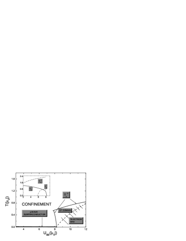
Figure 1: The phase diagram of the CFs in the $U_{BB}$-$T$ plane for $n^{a}=1$, $U_{BF}=U_{BB}/2$ $\bar{t}_{F}=\sqrt{60}$, $n^{f}=0.55$. The solid curves are the critical temperature $T^{1*}_{c}$ after considering the gauge fluctuation and the shrink of the CF Fermi surface. The dash lines and the slashed area is the crossover from the ’electron’ gas to the CF domain. The inset is the mean field phase diagram for both bosons and fermions.

The density-density response function $\Pi^{B(0)}_{00}$ of free slave boson yields an effective attraction between CFs in the long wave length limit. This means that the UMF state is not stable if $t_{B}$ term does not contribute to $\Pi^{B}_{00}$, which is indeed the case in the BSF phase. In the MI, the $t_{B}$ term may be thought as a perturbation if $U_{BB}$ and $|U_{BB}-U_{BF}|$ are much larger than $t_{B}$. For the $n^{a}_{i}=1$ MI phase, the second order perturbation and the MI character, $n^{c}_{1i}+n^{h}_{1i}=1$, $t_{B}$ terms contribute an effective interaction between the CFs or slave bosons

$${\cal J}=\sum_{i\neq j}J_{ij}n^{c}_{i}n^{c}_{j}+{\rm const}=\sum_{i\neq j}J_{ij}n^{h}_{i}n^{h}_{j}+{\rm const^{\prime}},$$ (9)

with $J_{ij}=\frac{16t_{B,ij}^{2}U_{BF}^{2}}{U_{BB}(U_{BB}^{2}-U_{BF}^{2})}$. We see that this interaction is attractive if $U_{BF}>U_{BB}$ while it is repulsive if $U_{BF}<U_{BB}$. For the repulsive one, if $t_{B,ij}=t_{B}/\sqrt{|{\bf r}_{i}-{\bf r}_{j}|}$ for a special spatial structure, the effective interaction between CF or the slave boson in the continuous limit is a pure Coulomb one ${\cal J}=\sum_{k,k^{\prime},q}V(q)c^{\dagger}_{{\bf k}+{\bf q}}c_{\bf k}c^{\dagger}_{{\bf k^{\prime}}-{\bf q}}c_{\bf k^{\prime}}=\sum_{k,k^{\prime},q}V(q)h^{\dagger}_{{\bf k}+{\bf q}}h_{\bf k}h^{\dagger}_{{\bf k^{\prime}}-{\bf q}}h_{\bf k^{\prime}}$ with

$$V(q)=\frac{4\pi e^{2}}{q^{2}},$$ (10)

and the ’charge’ of the CF is defined by $e^{2}=\frac{16t_{B}^{2}U_{BF}^{2}}{U_{BB}(U_{BB}^{2}-U_{BF}^{2})}$. This repulsive interaction keeps the stability of the UMF state against the gauge fluctuations. Eq. (10) means that the CFs in the MI phase behave like ’electrons’. ’Electrons’ are a Coulomb gas. Notice that the electron gas at the half filling ($n^{f}=1/2$) turns to a checkerboard ’electron’ lattice. In this way, we see that the ’electron’ and ’photon’ (the gauge field) emerge from a neutral SUSY particle model.

In the ulrtacold Bose-Fermi mixture, instead of a pure Coulomb interaction caused by a long range hopping $t_{B,ij}$, the interaction between nearest neighbor sites dominates which is caused by $t_{B,ij}=t_{B}\neq 0$ if only $(i,j)$ is a nearest neighbor pair. The interaction between CFs at $T=0$ is given by $V(q)=\frac{32\pi t_{B}^{2}U_{BF}^{2}}{U_{BB}(U_{BB}^{2}-U_{BF}^{2})}$. (Also see comp .)

According to these discussions, we now may figure out the phase diagram of the CF in Fig. 1. The mean field phase transition temperature $T_{c}^{1}$ is suppressed greatly to $T_{c}^{1*}$ which is determined by the $T_{c}$ and $T_{p}$. The dash line is the estimated crossover line from the ’electron’ gas (the MI of bosons) to CF domains which arises from the effective attraction between CFs. In the BSF, the induced attraction between CFs, $(\Pi^{B(0)}_{00}(q,0))^{-1}\sim-\frac{m_{B}q^{2}}{\rho_{0}}$, may lead to a $p$ wave superconducting ground state. However, this might be difficult to reach in the ultracold mixture you .

The experimental implications of the UMF phase are discussed as follows. We consider the ’electron’ response to an external ’electric’ field, ’made’ by a change of the lattice potential of the fermions. This disturbs the density of fermions with $H^{\prime}(t)=-\sum_{i}n^{f}({\bf r}_{i},t)\varphi({\bf r}_{i},t)$. In a time flying experiment, the difference between disturbed and undisturbed fermion densities by external field is given by $n_{f}({\bf r})-n^{0}_{f}({\bf r})=(\frac{m_{f}}{t})|\tilde{w}_{f}({\bf k}=\frac{m_{f}{\bf r}}{t})|^{2}\delta n_{f}({\bf k}=\frac{m_{f}{\bf r}}{t})$ where $t$ is the flying time, $\tilde{w}_{f}$ is the Fourier component of the fermion Wannier function and $\delta n_{f}({\bf k})\propto\Pi_{00}({\bf k},0)$ . If $T>T_{c}^{1*}$, the density response of the system is simply given by the free fermion one, $\Pi^{F(0)}_{00}$. For $T<T^{1*}_{c}$, since $n^{f}\approx n_{c}^{1}$, the two CF response function is given by $\Pi_{00}^{-1}=(\Pi^{F(0)}_{00})^{-1}+(\Pi^{B(0)}_{00})^{-1}$. Negative $\Pi^{B(0)}_{00}$ leads to the instability of the CF. However, near the MI, the RPA gives $\Pi_{00}^{-1}=(\Pi^{F(0)}_{00})^{-1}+(\Pi^{B(0)}_{00})^{-1}+V(q)$. The repulsive between CFs stabilizes the CF against the gauge fluctuation. A better experimentally measurable quantity is the visibility ${\cal V}=\frac{n_{f}({\bf r}_{\rm max})-n_{f}({\bf r}_{\rm min})}{n_{f}({\bf r}_{\rm max})+n_{f}({\bf r}_{\rm min})}$ where ${\bf r}_{\rm max}$ and ${\bf r}_{\rm min}$ are chosen such that the Wannier envelop is cancelled vi . The difference between the disturbed and undisturbed visibility may directly correspond to the response function because $n_{f}({\bf r}_{\rm max})+n_{f}({\bf r}_{\rm min})\approx n^{0}_{f}({\bf r}_{\rm max})+n^{0}_{f}({\bf r}_{\rm min})$ in denominator.

The Fermi surface of pure cold fermions has been observed in a recent experiment kms by the time flying experiment. We suggest to do the same observation to the mixture. It is expected that instead of the constitution fermion’s Fermi surface, one may observe the ’electron’ Fermi surface in the ’electron’ gas.

In conclusions, we deduced the low energy physics of the SUSY Hubbard model. The ’electron’ and ’photon’, as well as the Higgs boson, were thought as emergent objects. The phase diagram was depicted, which showed what happened as the temperature was from high to low. Possible experiments to verify this theory were suggested by means of the cold Bose-Fermi atom mixture. We expect to generalize our theory to include a non-abelian gauge field wl coupled to fermions with spin degrees of freedom. However, it will not be a simple generalization of the $U(1)$ theory. Many problems, such as quark asymptotic free in an ultraviolet limit and confinement at low energy, have to be solved. The origin of the chiral fermions in $SU(2)\times U(1)$ weak-electric interaction is also non-trivial. We expect a relativistic version of the present theory.

This work was supported in part by Chinese National Natural Science Foundation and the NSF of USA.

References

• (1) For a possible origin of the electron and photon , see, e.g., P. A. Lee, N. Nagaosa, X. G. Wen, to be published in Rev. Mod. Phys. ( see, cond-mat/0410445).
• (2) M. Sneok, M. Haque, S. Vandoren, and H. T. C. Stoof, cond-mat/0505055.
• (3) A. Albus, F. Illuminati, J. Eisert, Phys. Rev. A 68, 023606 (2003).
• (4) M. Lewenstein, L. Santos, M. A. Baranov, and H. Fehrmann, Phys. Rev. Lett. 92, 050401 (2004).
• (5) G. Modugno et al, Phys. Rev. A. 68, 011601(R) (2003). C. Schori et al, Phys. Rev. Lett 93, 240402 (2004). S. Inouye et al, Phys. Rev. Lett. 93, 183201 (2004). J. Goldwin et al, Phys. Rev. A 70, 021601(R) (2004).
• (6) C. A. Stan et al, Phys. Rev. Lett. 93 143001 (2004).
• (7) M. Köhl et al, Phys. Rev. Lett. 94, 080403 (2005).
• (8) L. B. Ioffe and A. I. Larkin, Phys. Rev. B 39, 8988 (1989).
• (9) D. B. Dickerscheid, D. van Oosten, P. J. H. Densteneer, and H. T. C. Stoof, Phys. Rev. A 68, 043623(2003).
• (10) Yue Yu and S. T. Chui, Phys. Rev. A 71, 033608(2005).
• (11) X. C. Lu, J. B. Li, and Y. Yu, cond-mat/0504503.
• (12) I. Affleck and J. B. Marston, Phys. Rev. B 37, 3774 (1988).
• (13) X. G. Wen and P. A. Lee, Phys. Rev. Lett. 76, 503 (1996).
• (14) L. You and M. Marinescu, Phys. Rev. A 60, 2324 (1999).
• (15) F. Gerbier, A. Widera, S. Fölling, O. Mandel, T. Gericke, and I. Bloch, Phys. Rev. Lett. 95, 050404 (2005).