Magnetic field induced finite size effect in type-II superconductors

Abstract

We explore the occurrence of a magnetic field induced finite size effect on the specific heat and correlation lengths of anisotropic type-II superconductors near the zero field transition temperature $T_{c}$. Since near the zero field transition thermal fluctuations are expected to dominate and with increasing field strength these fluctuations become one dimensional, whereupon the effect of fluctuations increases, it appears unavoidable to account for thermal fluctuations. Invoking the scaling theory of critical phenomena it is shown that the specific heat data of nearly optimally doped YBa₂Cu₃O_7-δ are inconsistent with the traditional mean-field and lowest Landau level predictions of a continuous superconductor to normal state transition along an upper critical field $H_{c2}\left(T\right)$. On the contrary, we observe agreement with a magnetic field induced finite size effect, whereupon even the correlation length longitudinal to the applied field $H$ cannot grow beyond the limiting magnetic length $L_{H}$ $\propto\sqrt{\Phi_{0}/H}$. It arises because with increasing magnetic field the density of vortex lines becomes greater, but this cannot continue indefinitely. $L_{H}$ is then roughly set on the proximity of vortex lines by the overlapping of their cores. Thus, the shift and the rounding of the specific heat peak in an applied field is traced back to a magnetic field induced finite size effect in the correlation length longitudinal to the applied field.

The superconductor to normal state transition in conventional low $T_{c}$ materials appears to be well described by the Ginzburg-Landau mean-field approximation. Because of the large correlation volume in these materials, the region in which critical fluctuations are important is too small to be accessible experimentally. In contrast, with the discovery of superconductivity in the cuprates, a new era started [1]. Indeed, marked deviations from mean-field behavior have been observed over a temperature range of the order of $10$ K above and below $T_{c}$ [2, 3, 4, 5, 6, 7, 8, 9, 10, 11, 12, 13, 14, 15, 16, 17, 18, 19, 20, 21, 22]. Theoretical expectations of the kind of critical behavior which might be observed are: (i) If fluctuations in the vector potential can be ignored, then the zero-field transition belongs to the universality class of the three dimensional XY-model, as is the superfluid transition in ⁴He. In an applied magnetic field the critical behavior is then equivalent to that of uniformly rotating ⁴He near the superfluid transition [22, 23]; (ii) When fluctuations in the vector potential are included  the charge of the Cooper pairs, entering via the effective dimensionless charge $\widetilde{e}=\xi/\lambda=1/\kappa$, charged critical behavior is expected to occur in which both the correlation length $\xi$ and the magnetic penetration depth $\lambda$ grow with the same critical exponent by approaching $T_{c}$ from below [24, 25, 26, 27, 28, 29, 30, 31, 32, 33]. However, in extreme type-II superconductors where $\kappa>>1$ the effective charge $\widetilde{e}$ is very small. As a consequence the region close to $T_{c}$, where the system crosses over to the regime of charged fluctuations, becomes too narrow to access. For instance, optimally doped YBa₂Cu₃O_7-δ, while possessing an extended regime of critical fluctuations, is too strongly type-II to observe charged critical fluctuations [2, 3, 4, 5, 6, 7, 8, 9, 10, 11, 12, 13, 14, 15, 16, 17, 18, 19, 20, 21, 22]. In strongly type-II superconductors ($\kappa\ >>1$) the crossover upon approaching $T_{c}$ is thus initially to the critical regime of a weakly charged superfluid where the fluctuations of the order parameter are essentially those of an uncharged superfluid or XY-model. Furthermore, there is the inhomogeneity induced finite size effect which renders the asymptotic critical regime unattainable [20, 21]. However, underdoped cuprates appear to open a window onto the charged critical regime because $\kappa$ becomes rather small in this doping regime. Here the cuprates undergo a quantum superconductor to insulator transition in the underdoped limit [16, 22] and correspond to a 2D disordered bosonic system with long-range coulomb interactions. Close to this quantum transition $T_{c}$, $\lambda_{ab}$ and $\xi_{ab}$ scale as $T_{c}\propto\lambda_{ab}^{-2}$ $\propto\xi_{ab}^{-z}$ [16, 22], yielding with the dynamic critical exponent $z=1$ [16, 22, 34, 35, 36], $\kappa_{ab}\propto\sqrt{T_{c}}$. Recent measurements of the magnetic in-plane penetration depth of underdoped YBa₂Cu₃O_6.59 clearly uncovered critical behavior associated with a charged critical point, in which both the coherence length and the magnetic penetration depth grow by approaching $T_{c}$ from below with the same critical exponent [37]. Thus, as far as static zero field critical phenomena are concerned, there is little doubt that near optimum doping the observable critical behavior of bulk YBa₂Cu₃O_7-δ is governed by the three dimensional(3D) XY universality class. Accordingly, we expect that the critical behavior in an applied magnetic field is equivalent to that of uniformly rotating ⁴He near the superfluid transition [22, 23]. The singular part of the free energy per unit volume should then scale as [16, 22]

$$f_{s}=\frac{Q^{\pm}k_{B}T\gamma}{\left(\xi_{ab}^{\pm}\right)^{3}}G\left(z\right),\text{ }z=\frac{H_{c}\left(\xi_{ab}^{\pm}\right)^{2}}{\Phi_{0}},\xi_{ab}^{\pm}=\xi_{ab0}^{\pm}\left|t\right|^{-\nu},G^{\pm}\left(0\right)=1,$$ (1)

for a magnetic field $H_{c}$ applied parallel to the $c$-axis. $G\left(z\right)$ is a universal scaling function, $\pm=sgn\left(t\right)=sgn\left(T/T_{c}-1\right)$, $\xi_{ab}^{\pm}$ the zero-field in-plane correlation length with critical amplitude $\xi_{ab0}^{\pm}$, $\gamma=\xi_{ab0}^{\pm}/\xi_{c0}^{\pm}$ the anisotropy, and $Q^{\pm}$ is  a universal constant, fixed by the 3D-XY universality class. The fluctuation contribution to the magnetization $m=-\partial f_{s}/\partial H_{c}$ scales then as

$$\frac{m\left(H_{c},T\right)}{TH_{c}^{1/2}}=-\frac{Q^{\pm}k_{B}\gamma}{\Phi_{0}^{3/2}}z^{-1/2}\frac{dG}{dz},$$ (2)

while the singular part of the specific heat, $\widetilde{c}\left(H_{c},T\right)=c\left(H_{c},T\right)\rho/k_{B}\simeq-\partial^{2}f_{s}/\partial\left|t\right|^{2}$ adopts the scaling form

$$\widetilde{c}\left(H_{c},T\right)=\frac{A^{\pm}}{\alpha}\left|t\right|^{-\alpha}F^{\pm}\left(z\right),~{}\frac{A^{\pm}\left(\xi_{ab0}^{\pm}\right)^{3}}{\gamma}=-Q^{\pm}\alpha\left(1-\alpha\right)\left(2-\alpha\right)=\left(R^{\pm}\right)^{3},~{}3\nu=2-\alpha,$$ (3)

where

$$F^{\pm}\left(z\right)=G^{\pm}\left(z\right)-\frac{2\left(4\nu+1\right)}{3\left(3\nu-1\right)}z\frac{dG^{\pm}\left(z\right)}{dz}+\frac{4\nu}{3\left(3\nu-1\right)}z^{2}\frac{d^{2}G^{\pm}\left(z\right)}{dz^{2}}.$$ (4)

$\rho$ denotes the density and $c\left(H_{c},T\right)$ is in units of $\left(erg/\left(gK\right)\right)$. In the 3D-XY universality class are the universal quantities $Q^{\pm}$, $R^{\pm}$, $\nu$ and $\alpha$ given by [38]

$$R^{+}\simeq 0.36,\text{ }R^{-}\simeq 0.82,\text{ }A^{+}/A^{-}\simeq 1.06,\text{ }\frac{\xi_{ab0,c0}^{-}}{\xi_{ab0,c0}^{+}}\simeq 2.28,\text{ }\nu=\left(2-\alpha\right)/3\simeq 0.67$$ (5)

In the presence of a sufficiently small magnetic field $H_{c}$, the specific heat is then expected to have a singular part which exhibits the scaling behavior

$$\widetilde{c}\left(H_{c},T\right)=\frac{A^{\pm}}{\alpha}\left(\frac{H_{c}\xi_{ab0}^{2}}{\Phi_{0}}\right)^{-\alpha/2\nu}z^{-\alpha/2\nu}F^{\pm}\left(z\right)=\frac{A^{\pm}}{\alpha}\left(\frac{H_{c}\xi_{ab0}^{2}}{\Phi_{0}}\right)^{-\alpha/2\nu}x^{-\alpha}F^{\pm}\left(x^{-1/2\nu}\right),\text{ }x=z^{-1/2\nu}.$$ (6)

The magnetization data [5, 10] and the zero-field specific heat measurements of YBa₂Cu₃O_7-δ [4, 9, 16] agree well with these predictions. In a nonzero applied field, one can test the scaling form (6) of the specific heat by the extent to which data for $\widetilde{c}\left(H_{c},T\right)H_{c}^{\alpha/2\nu}$ collapse to a common curve when plotted as a function of $x$. Here, matters are complicated by the fact that a different kind of scaling behavior

$$\widetilde{c}\left(H_{c},T\right)=R\left(x_{L}\right),\text{ }x_{L}=\frac{T-T_{c2}\left(H_{c}\right)}{\left(TH_{c}\right)^{2/3}},$$ (7)

is expected when only the lowest Landau level ($L$) is significantly occupied [39, 40]. Here $T-T_{c2}\left(H_{c}\right)$, or equivalently, $H_{c}=H_{c2}\left(T\right)$ is the upper critical field of the Ginzburg-Landau theory. Since $\alpha$ in Eq.(6) is very small, and $2\nu\approx 4/3$, the two predictions are rather hard to distinguish [41]. Some authors argue that lowest-Landau-level scaling works just as well as critical-point scaling [42, 43, 44, 45, 46, 47, 48, 49, 50, 51, 52].

Theoretically, the scaling form (6) is an unambiguous prediction of the theory of critical phenomena and ought to be observed sufficiently close to the zero-field critical point. On the other hand, lowest-Landau-level scaling, relies on the assumption that the correlation length longitudinal to the applied magnetic field, diverges along the line $T_{c2}\left(H\right)$ [53], whereupon a continuous phase transition from the superconducting to the normal state is predicted to occur. Accordingly, the behavior of the correlation length longitudinal to the applied field is essential to verify the lowest Landau level prediction. In this context it is instructive to rewrite the scaling variable $z$ (Eq.(1)) in the form

$$z=\frac{H_{c}\xi_{ab}^{2}}{\Phi_{0}}=\frac{\xi_{ab}^{2}}{aL_{H_{c}}^{2}},\text{ }L_{H_{i}}=\sqrt{\Phi_{0}/\left(aH_{i}\right)},$$ (8)

with $a\simeq 3.12$[20], related to the average distance between vortex lines [20, 22, 54, 55, 56]. The scaling function $G\left(z\right)$ is then identical to that of a system with finite extent $L_{H_{c}}$ in the $ab$-plane [57, 58]. As a consequence, fluctuations which are transverse to the applied field are stiff and the corresponding correlation lengths cannot grow beyond

$$\sqrt{\xi_{i}^{-}\xi_{j}^{-}}=\sqrt{\Phi_{0}/\left(aH_{k}\right)}=L_{H_{k}},\ i\neq j\neq k.$$ (9)

Hence, the fluctuations of a bulk superconductor in a magnetic field are longitudinal to the field and for this reason one dimensional, as noted by Lee and Shenoy [59]. Noting that fluctuations become more important with reduced dimensionality, one expects that the remaining fluctuations, which are longitudinal to the applied field, remove the mean-field transition at $T_{c2}\left(H_{c}\right)$. Indeed, thermal fluctuations destroy the ordered phase in one dimensional systems with short-range interactions. Furthermore, calculations treating these interactions within the Hartree approximation [39, 40, 54, 60], and generalizations thereof [41, 61, 62], find that the correlation length longitudinal to the applied field remains bounded as well. In this case the correlation length $\xi_{c}^{-}\left(H_{c},t\right)$ adopts the scaling form

$$\xi_{c}\left(H_{c},t\right)=\xi_{c0}^{\pm}\left|t\right|^{-\nu}S^{\pm}\left(x\right),\text{ }x=\left(\frac{H_{c}\gamma^{2}\left(\xi_{c0}^{-}\right)^{2}}{\Phi_{0}}\right)^{-1/2\nu}\left|t\right|.$$ (10)

The scaling function must behave as

$$S^{\pm}\left(x=\pm\infty\right)=1,\text{ \ }S^{\pm}\left(x\rightarrow\pm 0\right)=s_{0}\left|x\right|^{\nu},$$ (11)

so that for $H_{c}\rightarrow 0$, $\xi_{c}\left(H_{c},t\right)\propto\left|t\right|^{-\nu}$ and for $t\rightarrow 0$, $\xi_{c}\left(H_{c},t\right)\propto\sqrt{\Phi_{0}/H_{c}\text{ }}$. Thus, the divergence of the correlation length $\xi_{c}^{-}\left(H_{c},t\right)$ is removed and it adopts a maximum at $T_{p}\left(H_{c}\right)$ $<T_{c}$, yielding the line

$$H_{pc}\left(t\right)=\frac{\Phi_{0}}{x_{p}^{2\nu}\left(\xi_{ab0}^{-}\right)^{2}}\left|t\right|^{2\nu}.$$ (12)

On the other hand, the specific heat scales according to Eq.(3) as

$$\widetilde{c}\left(H_{c},t\right)=\frac{A^{\pm}}{\alpha}\left|t\right|^{-\alpha}F^{\pm}\left(x\right).$$ (13)

In this case the scaling function behaves as

$$F^{\pm}\left(x=\pm\infty\right)=1,\text{ }F^{\pm}\left(x=\pm 0\right)=f_{\pm}\left|x\right|^{\alpha},$$ (14)

so that for $H_{c}\rightarrow 0$, $\widetilde{c}\left(H_{c},t\right)\propto\left|t\right|^{-\alpha}$ and for $t\rightarrow 0$, $\widetilde{c}\left(H_{c},t\right)\propto\left(\Phi_{0}/H_{c}\right)^{-\alpha/2\nu}$. Noting that the ratio $S^{\pm}\left(x\right)/\left(F^{\pm}\left(x\right)\right)^{\nu/\alpha}$ tends to constant values in the limits $x\rightarrow 0$ and $x\rightarrow\pm\infty$ the relation between the $\xi_{c}\left(t,H_{c}\right)$ and the absolute value of the specific heat $\left|\widetilde{c}\left(H_{c},T\right)\right|$,

$$\xi_{c}\left(H_{c},t\right)=\xi_{c0}^{\pm}\left|\frac{A^{\pm}}{\alpha}\right|^{-\nu/\alpha}\left|\widetilde{c}\left(H_{c},t\right)\right|^{\nu/\alpha}\frac{S^{\pm}\left(x\right)}{\left(F^{\pm}\left(x\right)\right)^{\nu/\alpha}},$$ (15)

as obtained from Eqs.(10) and (13), reduces in these limits to

$$\xi_{c}\left(H_{c},t\right)\propto\left|\widetilde{c}\left(H_{c},t\right)\right|^{\nu/\alpha}.$$ (16)

Thus, when this scenario holds true, the specific heat probes essentially the correlation length longitudinal to the applied field. As a remnant of the singularity at $T_{c}$ in zero field it should exhibit a so called finite size effect [57, 58], resulting in a smooth peak around $T_{p}$ because the correlation length $\xi_{c}\left(t,H_{c}\right)$ cannot grow beyond $\xi_{c}\left(t_{p},H_{c}\right)$ (Eq.(12)). Furthermore, given experimental data for $\widetilde{c}\left(H_{c},t\right)$, this scenario can be verified. Indeed in the limits $H_{c}\rightarrow 0$ and $t\rightarrow\pm 0$ the critical behavior $\left|\widetilde{c}\left(H_{c},t\right)\right|^{\nu/\alpha}\propto\xi_{c0}^{\pm}\left|t\right|^{-\nu}$ with $\xi_{c0}^{-}/\xi_{c0}^{+}\simeq 2.28$ (Eqs.(5)) should hold. This allows to circumvent the aforementioned difficulties associated with the comparison of scaling functions with the prediction of the lowest-Landau-level approach. Indeed, if there is a magnetic field induced finite size effect on the correlation length longitudinal to the applied field, the transition is rounded and the assumption of an upper critical field $H_{c2}$ is not justified.

Here we analyze the specific heat data of Roulin et al. [49] to verify the magnetic field induced finite size scenario. In Fig.1a we depicted the data for the YBa₂Cu₃O_7-δ single crystal in terms of $\widetilde{c}\left(H_{c},t\right)\propto c\left(H_{c},T\right)/T-B$ vs. $t=T/T_{c}-1$ with $B=0.1717$ J/K²gat  and $T_{c}=92.77$ K. The solid and dashed lines are $\widetilde{c}\left(H_{c},t\right)\propto c\left(H_{c},T\right)/T-B=\widetilde{A}^{\pm}\left|t\right|^{-\alpha}$ with $\widetilde{A}^{-}=-0.0672$ J/K²gat, $\widetilde{A}^{+}=-0.0685$ J/(K²gat), and $\alpha=-0.01$ (Eq.(5)). Using the relations $A^{-}\left(\text{J/(K gat)}\right)=$ $\widetilde{A}^{-}T_{c}\alpha$, $A^{-}\left(cm^{-3}\right)=10^{7}/\left(k_{B}V_{gat}\right)A^{-}\left(\text{J/(K gat)}\right)$, and $V_{gat}=8$ cm³ we obtain for $A^{-}$ the estimate $A^{-}=5.64$ $10^{20}$ cm^-3 and with the universal relations (3) and (5) for the correlation volume and the critical amplitudes of the zero field correlation lengths the estimates

$$\left(\xi_{ab0}^{-}\right)^{2}\xi_{c0}^{-}\simeq 978\text{ \AA}^{3},\xi_{ab0}^{-}\simeq 18.43\text{ \AA},\text{ }\xi_{c0}^{-}\simeq 2.88\text{ \AA,}$$ (17)

using $\gamma=6.4$.  As a remnant of the zero-field singularity, there is for fixed field strength a smeared peak adopting its maximum at $T_{p}$ which is located below $T_{c}$. As $T_{p}$ approaches $T_{c}$, the peak becomes sharper with decreasing $H_{c}$ and evolves smoothly to the zero-field behavior, smeared by the inhomogeneity induced finite size effect, arising from the limited extent $L_{ab,c}$ of the homogeneous domains along the $ab$-plane and $c$-axes. Since $T_{p}$ decreases systematically with reduced field down to $H_{c}=0.25$ T, corresponding to $L_{H_{c}}\leq\sqrt{\Phi_{0}/\left(aH_{c}\right)}=512$ Å, the magnetic field sets at and above $H_{c}=0.25$ T the limiting length. On the contrary, when $L_{H_{c}}\geq L_{ab}$, the inhomogeneities set the limiting length. In this case, $t_{p}=\left(\xi_{ab0}^{-}/L_{ab}\right)^{1/\nu}$, independent of the applied field. Thus, the field dependence of $t_{p}$ is a characteristic feature of a magnetic field induced limiting length. The line $H_{cp}\left(t\right)$ is shown in Fig.1b. The solid line is Eq.(12) with $\Phi_{0}/\left(x_{p}^{2\nu}\left(\xi_{ab0}^{-}\right)^{2}\right)=210$ T, yielding with $\xi_{ab0}^{-}\simeq 18.43$ Å (Eq.(17)),

$$x_{p}\simeq 2.21,$$ (18)

and $z_{p}=x_{p}^{-1/2\nu}\simeq 0.55$, which agrees well with the previous estimate $z_{p}\simeq a^{-1/2}=3.12^{-1/2}\simeq 0.57$ [20].

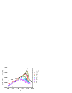
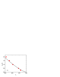
FIG. 1.: a) $\widetilde{c}\left(H_{c},t\right)\propto c\left(H_{c},T\right)/T-B$ vs. $t$ for YBa₂Cu₃O_7-δ derived from Roulin et al. [49] with $B=0.1717$ J/K²gat  and $T_{c}=92.77$ K; The solid and dashed lines are $\widetilde{c}\left(H_{c},t\right)\propto c\left(H_{c},T\right)/T-B=\widetilde{A}^{\pm}\left|t\right|^{-\alpha}$ with $\widetilde{A}^{-}=-0.0671$ J/K²gat, $\widetilde{A}^{+}=-0.0684$ J/K²gat, and $\alpha=-0.01$. b) $H_{cp}\left(t\right)$ vs. $t$ . The solid line is $H_{cp}\left(t\right)=210\left|t\right|^{2\nu}$ with $\nu=0.67$, corresponding to Eq.(12) with $\Phi_{0}/\left(x_{p}^{2\nu}\left(\xi_{ab0}^{-}\right)^{2}\right)=210$ (T).

In Fig.2 we displayed the scaling plot $\widetilde{c}\left(H_{c},t\right)\left|t\right|^{\alpha}\propto\left(c\left(H_{c},T\right)/T-B\right)\left|t\right|^{\alpha}$ vs. $t/H_{c}^{1/2\nu}$ derived from the data of Roulin et al. [49] shown in Fig.1a. Noting that according to Eq.(13), $\left(c\left(H_{c},T\right)/T-B\right)\left|t\right|^{\alpha}\propto\widetilde{c}\left(H_{c},t\right)\left|t\right|^{-\alpha}=A^{\pm}F^{\pm}\left(x\right)/\alpha$, where $x\propto t/H_{c}^{1/2\nu}$, this plot uncovers essentially the scaling function $F^{\pm}\left(x\right)$, whereupon the data points should fall on a single curve, as they apparently do, when plotted versus $x\propto t/H_{c}^{1/2\nu}$. The solid and dashed curves indicate the asymptotic behavior in the limits $x\propto t/H_{c}^{1/2\nu}\rightarrow\pm 0$ (Eq.(14)), while the arrow marks $t_{p}/H_{c}^{1/2\nu}=x_{p}\left(\left(\xi_{ab0}^{-}\right)^{2}/\Phi_{0}\right)^{1/2\nu}$, where the peak in the specific heat adopts its maximum value. However, as aforementioned, it is difficult to distinguish different models on the basis of such scaling functions.

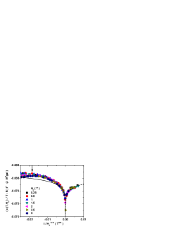
FIG. 2.: $\widetilde{c}\left(H_{c},t\right)\left|t\right|^{-\alpha}\propto\left(c\left(H_{c},T\right)/T-B\right)\left|t\right|^{\alpha}$ vs. $t/H_{c}^{1/2\nu}$ derived from the data of Roulin et al. [49] shown in Fig.1a. The solid and dashed lines are $-0.0654\left(-t/H_{c}^{1/2\nu}\right)^{\alpha}$ and $-0.0658\left(-t/H_{c}^{1/2\nu}\right)^{\alpha}$, respectively. The arrow marks $t_{p}/H^{1/2\nu}\simeq-0.0184$.

However, in view of Eqs.(15) and (16), giving the relationship between the fluctuation contribution to the specific heat and the correlation length longitudinal to the applied field, $\xi_{c}\left(t,H_{c}\right)$, the magnetic field induced finite size scenario can be verified by considering the plot $\left|\widetilde{c}\left(H_{c},t\right)\right|^{\nu/\alpha}\propto\left|c\left(T,H_{c}\right)/T-B\right|^{\nu/\alpha}$ vs. $t$, predicted to probe $\xi_{c}\left(t,H_{c}\right)$. In Fig.3 we show $\left|\widetilde{c}\left(H_{c},t\right)\right|^{\nu/\alpha}\propto\left|c\left(T,H_{c}\right)/T-B\right|^{\nu/\alpha}$ vs. $t$ derived from the data of Roulin et al. [49] shown in Fig.1a. The solid and dashed line mark the leading zero field critical behavior in terms of $\left|\widetilde{c}\left(H_{c},t\right)\right|^{\nu/\alpha}\propto\left|c\left(T,H_{c}\right)/T-B\right|^{\nu/\alpha}=\Gamma^{\pm}\left|t\right|^{-\nu}$, with $\Gamma^{-}/\Gamma^{+}=2.28$, consistent with the universal ratio $\xi_{c0}^{-}/\xi_{c0}^{+}\simeq 2.28$ of the 3D-XY universality class (Eq.(5)). This confirms that in the scaling regime considered here $\left|\widetilde{c}\left(H_{c},t\right)\right|^{\nu/\alpha}$ probes essentially the correlation length longitudinal to the applied magnetic field, $\xi_{c}\left(t,H_{c}\right)$, so that Eq.(16) applies. The rounded peak in zero field reveals then an inhomogeneity induced finite size effect, while the smeared peak in finite fields, its shift and broadening with increasing field strength discloses the magnetic field induced finite size effect on the correlation length longitudinal to the applied field. Because $\xi_{c}\left(t,H_{c}\right)\propto\left|\widetilde{c}\left(H_{c},t\right)\right|^{\nu/\alpha}\propto\left|c\left(T,H_{c}\right)/T-B\right|^{\nu/\alpha}$ the field dependence of $t_{p}$, where the correlation length adopts its maximum value set by the magnetic field, coincides with the $t_{p}\left(H_{c}\right)$, where the specific heat reaches its maximum value. In this context it is important to recognize that the magnetic field dependence of $t_{p}$ is a unique consequence of the magnetic field induced finite size effect. Indeed, when inhomogeneities set the limiting length then $t_{p}=\left(\xi_{ab0}^{-}/L_{ab}\right)^{1/\nu}$, independent of the applied field.

When the magnetic field induced finite size effect scenario is correct, the occurrence of the effect is not restricted to temperatures below $T_{c}$.  It is particularly dramatic at $T_{c}$, where in a homogeneous system in zero field the correlation lengths are infinite. In an applied field the scaling form (10) yields the prediction

$$\xi_{c}\left(H_{c},t=0\right)=\frac{s_{0}}{\gamma}\left(\frac{\Phi_{0}}{H_{c}}\right)^{1/2}=\frac{s_{0}a^{1/2}}{\gamma}L_{H_{c}},$$ (19)

where we used the definition (8 for the limiting magnetic length $L_{H_{c}}$. In Fig.3b we displayed $\xi_{c}\left(H_{c},t=0\right)\propto\left|\widetilde{c}\left(H_{c},t=0\right)\right|^{\nu/\alpha}\propto\left|c\left(H_{c},T_{c}\right)/T_{c}-B\right|^{\nu/\alpha}$ vs. $H_{c}$. The consistency with the solid line, which is Eq.(19) in the form $\xi_{c}\left(H_{c},t=0\right)\propto\left|\widetilde{c}\left(H_{c},t=0\right)\right|^{\nu/\alpha\propto}\left|c\left(H_{c},T_{c}\right)/T_{c}-B\right|^{\nu/\alpha}=3.210^{79}H_{c}^{-1/2}$, reveals again that an applied magnetic field leads to a finite size effect in the correlation length longitudinal to the field.

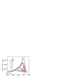
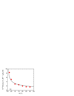
FIG. 3.: a) $\left|\widetilde{c}\left(H_{c},t\right)\right|^{\nu/\alpha}\propto\left|c\left(H_{c},T\right)/T-B\right|^{\nu/\alpha}$ vs. $t$ derived from the data of Roulin et al. [49] shown in Fig.1a. The solid and dashed lines are $\left|c\left(H_{c},T\right)/T-B\right|^{\nu/\alpha}=\Gamma^{\pm}\left|t\right|^{-\nu}$ with $\Gamma^{-}=4.7$ 10⁷⁸ , $\Gamma^{+}=\Gamma^{-}/2.28$ , and $\nu=0.67$. b) $\left|\widetilde{c}\left(H_{c},t=0\right)\right|^{\nu/\alpha}\propto\left|c\left(H_{c},T_{c}\right)/T_{c}-B\right|^{\nu/\alpha}$ vs. $H_{c}$ derived from the data shown in Fig.3a. The solid line is $\left|c\left(H_{c},T_{c}\right)/T_{c}-B\right|^{\nu/\alpha}=3.2$ $10^{79}H_{c}^{-1/2}$.

For fields applied parallel to the $a$-axis, the transverse correlation lengths $\xi_{b}$ and $\xi_{c}$ are according to Eq.(8) bounded by $\sqrt{\xi_{a}^{-}\xi_{b}^{-}}=L_{H_{a}}$. When the magnetic field induced finite size scenario holds true, the correlation length longitudinal to the applied field, $\xi_{a}\left(H_{a},t\right)$, should be bounded as well. In analogy to Eq.(10) the longitudinal correlation length adopts then the scaling form

$$\xi_{a}\left(H_{a},t\right)=\xi_{a0}^{\pm}\left|t\right|^{-\nu}S^{\pm}\left(x\right),\text{ }x=\left(\frac{H_{a}\xi_{b0}^{-}\xi_{c0}^{-}}{\Phi_{0}}\right)^{-1/2\nu}\left|t\right|,$$ (20)

with the limiting behavior given in Eq.(11). Thus, the divergence of the correlation length is removed and $\xi_{a}^{-}\left(H_{a},t\right)$ adopts at $T_{p}\left(H_{a}\right)$ $<T_{c}$ a maximum, yielding the line

$$H_{pa}\left(t\right)=\frac{\Phi_{0}}{x_{p}^{2\nu}\xi_{b0}^{-}\xi_{c0}^{-}}\left|t\right|^{2\nu}.$$ (21)

Furthermore, in analogy to Eq.(16) the relation

$$\xi_{a}\left(H_{a},t\right)\propto\left|\widetilde{c}\left(H_{a},t\right)\right|^{\nu/\alpha},$$ (22)

between the longitudinal correlation length and the specific heat should hold in the limits $x\rightarrow 0$ and $x\rightarrow\pm\infty$. In Fig.4a we depicted $\left|\widetilde{c}\left(H_{ab},t\right)\right|^{\nu/\alpha}\propto\left|c\left(H_{ab},T\right)/T-B\right|^{\nu/\alpha}$ vs. $t$ derived from the data of Roulin et al. [49]. The solid and dashed line mark the leading zero field critical behavior in terms of $\left|\widetilde{c}\left(H_{c},t\right)\right|^{\nu/\alpha}\propto\left|c\left(T,H_{c}\right)/T-B\right|^{\nu/\alpha}=\Gamma^{\pm}\left|t\right|^{-\nu}$, with $\Gamma^{-}/\Gamma^{+}=2.28$, consistent with the universal ratio $\xi_{ab0}^{-}/\xi_{ab0}^{+}\simeq 2.28$ of the 3D-XY universality class (Eq.(5)). This consistency confirms again that in the scaling regime considered here $\left|\widetilde{c}\left(H_{ab},t\right)\right|^{\nu/\alpha}$ probes the correlation length $\xi_{ab}\left(t,H_{ab}\right)$ longitudinal to the applied field. The rounded peak in zero field reveals an inhomogeneity induced finite size effect, while the smeared peak in finite fields, its shift and broadening with increasing field strength disclose the magnetic field induced finite size effect in $\xi_{ab}\left(t,H_{c}\right)$. Indeed, from Fig.4b it is seen that the field dependence of $t_{p}$ where the correlation length $\xi_{ab}\left(t,H_{c}\right)$ adopts its maximum value, set by the magnetic field, is consistent with $t_{p}=-0.0034H_{ab}^{1/2\nu}$ which is Eq.(21) with $\left(\left(x_{p}^{2\nu}\xi_{ab0}^{-}\xi_{c0}^{-}\right)/\Phi_{0}\right)^{1/2\nu}=0.0034$ (T), resulting from the $\xi_{ab,c0}^{-}$ given by Eq.(17) and $x_{p}=2.21$ (Eq.(18).

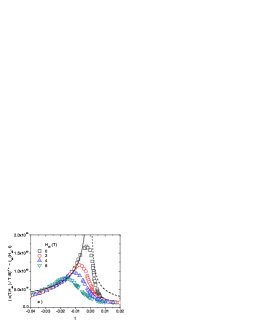
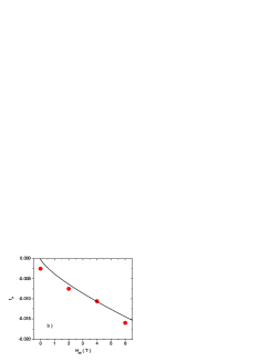
FIG. 4.: a) $\left|\widetilde{c}\left(H_{ab},t\right)\right|^{\nu/\alpha}\propto\left|c\left(H_{ab},T\right)/T-B\right|^{\nu/\alpha}$ vs. $t$ derived from the data of Roulin et al. [49] with $B=0.1717$ J/K²gat  and $T_{c}=92.77$ K. The solid and dashed lines are $\left|c\left(H_{ab},T\right)/T-B\right|^{\nu/\alpha}=\Gamma^{\pm}\left|t\right|^{-\nu}$ with $\Gamma^{-}=5.05$ 10⁷⁸ , $\Gamma^{+}=\Gamma^{-}/2.28$ , and $\nu=0.67$. b) $t_{p}$ vs. $H_{ab}$. The solid line is $t_{p}=-0.0034H_{ab}^{1/2\nu}$, which corresponds to Eq.(21) with $\left(\left(x_{p}^{2\nu}\xi_{ab0}^{-}\xi_{c0}^{-}\right)/\Phi_{0}\right)^{1/2\nu}=0.0034$ T.

To summarize our result for an anisotropic type-II superconductor, we have shown that near the zero field transition temperature superconductivity is in a magnetic field subjected to a field induced finite size effect. The crucial ingredient for a finite size effect is an energy gap in the excitation spectrum of fluctuations. In the present case it is the discrete set of Landau levels. Indeed, there is the formal analogy with the Landau levels of a charged particle moving in circular orbits in the plane perpendicular to the applied field at the cyclotron frequency. As a consequence, the fluctuations which are transverse to the field are stiff and have a length scale $L_{H}\propto\sqrt{\Phi_{0}/H}$. Hence, the fluctuations of a bulk type-II superconductor become one dimensional and are longitudinal to the applied field, as noted by Lee and Shenoy [59]. Because fluctuations become more important with reduced dimensionality, one expects then that the interaction of these fluctuations remove the mean-field transition at $T_{c2}\left(H_{c}\right)$, because thermal fluctuations destroy the ordered phase in one dimensional systems with short-range interactions. The absence of this transition is further supported by calculations treating the fluctuations within the Hartree approximation [39, 40, 54, 60], and generalizations thereof [41, 61, 62]. They suggest that the correlation length longitudinal to the applied field remains bounded as well. Invoking the scaling theory of critical phenomena we confirmed this prediction. We have shown that the specific heat data of Roulin et al. [51] clearly reveals a magnetic field induced finite size effect in the correlation length longitudinal to the applied field. Accordingly, there is no evidence for a phase transition line $T_{c2}\left(H\right)$ near the zero field transition temperature $T_{c}$.

REFERENCES

[1] J.G. Bednorz and K.A. M ller, Zeitschrift f r Physik, 64, 189
(1986).
[2] T. Schneider and D. Ariosa, Z. Phys. B 89, 267
(1992).
[3] T. Schneider and H. Keller, Int. J. Mod. Phys. B 8, 487 (1993).
[4] N. Overend, M.A. Howson, and I.D. Lawrie, Phys. Rev.
Lett. 72, 3238 (1994).
[5] M. A. Hubbard, M. B. Salamon, and B. W. Veal, Physica C
259, 309 (1996).
[6] Y. Jaccard, T. Schneider, J.-P. Locquet, E. J. Williams, P.
Martinoli and O. Fischer., Europhys. Lett., 34, 281 (1996).
[7] S. Kamal, D. A. Bonn, N. Goldenfeld, P. J. Hirschfeld, R.
Liang and W. N. Hardy., Phys. Rev. Lett. 73, 1845 (1994).
[8] S. Kamal, R. Liang, A. Hosseini, D. A. Bonn, and W. N.
Hardy, Phys. Rev. B 58, 8933 (1998).
[9] V. Pasler, P. Schweiss, Ch. Meingast, B. Obst, H. Wühl,
A. I. Rykov, and S. Tajima, Phys. Rev. Lett. 81, 1094
(1998).
[10] D. Babic, J. R. Cooper,J. W. Hodby and Chen Changkang,
Phys. Rev. B 60, 698 (1999).
[11] T. Schneider, J. Hofer, M. Willemin, J.M. Singer, and H.
Keller, Eur. Phys. J. B 3, 413 (1998).
[12] T. Schneider and J. M. Singer, Physica C 313, 188
(1999).
[13] J. Hofer, T. Schneider, J. M. Singer, M. Willemin, H. Keller,
Ch. Rossel, and J. Karpinski, Phys. Rev. B 60, 1332 (1999).
[14] J. Hofer, T. Schneider, J. M. Singer, M. Willemin, H.
Keller, T. Sasagawa, K. Kishio, K. Conder and J. Karpinski, Phys.
Rev. B 62, 631 (2000).
[15] T. Schneider and J. S. Singer, Physica C 341-348,
87 (2000).
[16] T. Schneider and J. M. Singer, Phase Transition
Approach To High Temperature Superconductivity, Imperial College
Press, London, 2000.
[17] Ch. Meingast, V. Pasler, P. Nagel, A. Rykov, S. Tajima,
and P. Olsson, Phys. Rev. Lett. 86, 1606 (2001).
[18] T. Schneider, Physica B 326, 289 (2003).
[19] K. D. Osborn, D. J. Van Harlingen, Vivek Aji, N.
Goldenfeld, S. Oh, and J. N. Eckstein, Phys. Rev. B 68,
144516 (2003).
[20] T. Schneider, Journal of Superconductivity, 17, 41
(2004).
[21] T. Schneider and D. Di Castro, Phys. Rev. B 69,
024502 (2004).
[22] T. Schneider, in: The Physics of Superconductors,
edited by K. Bennemann and J. B. Ketterson (Springer, Berlin,
(2004), p. 111.
[23] W. F. Vinen, in Superconductivity II, edited by R. D. Parks
(Marcel Dekker, INC., New York, 1969).
[24] C. Dasgupta and B. I. Halperin, Phys. Rev. Lett. 47, 1556 (1981).
[25] H. Kleinert, Lett. Nuovo Cimento 35, 405 (1982).
[26] S. Kolnberger and R. Folk, Phys. Rev. B 41,
4083 (1990).
[27] M. Kiometzis, H. Kleinert, and A. M. J. Schakel, Phys.
Rev. Lett. 73, 1975 (1994); Fortschr. Phys. 43,
697 (1995).
[28] I. F. Herbut and Z. Tesanovic, Phys. Rev. Lett. 76, 4588 (1996).
[29] I. F. Herbut, J. Phys. A 30, 423 (1997).
[30] P. Olsson and S. Teitel, Phys. Rev. Lett., 80,
1964 (1998).
[31] J. Hove and A. Sudbo, Phys. Rev. Lett., 84, 3426
(2000).
[32] J. Hove, S. Mo, and A. Sudbo, Phys. Rev. B 66,
064524 (2002).
[33] S.Mo, J. Hove, A. Sudbo, Phys. Rev. B 65, 104501
(2002).
[34] M.P.A. Fisher, G. Grinstein, and S. M. Girvin, Phys. Rev.
Lett. 64, 587 (1990.
[35] Min-Chul Cha, M. P. A. Fisher, M. Wallin, and A. P. Young,
Phys. Rev. B 44, 6883 (1991).
[36] I. F. Herbut, Phys. Rev. B 6, 14723 (2000).
[37] T. Schneider, R. Khasanov, K. Conder, E. Pomjakushina,
R. Bruetsch, and H. Keller, J. Phys.: Condens. Matter 16,
L1 (2004).
[38] A. Peliasetto and E. Vicari, Physics Reports 368,549 (2002).
[39] A.J. Bray, Phys. Rev. B 9, 4752 (1974).
[40] D.J. Thouless, Phys. Rev. Lett. 34, 946 (1975).
[41] Dominic J. Lee and Ian D. Lawrie, Phys. Rev. B 64, 184506 (2001).
[42] U. Welp, S. Fleshler, W.K. Kowk, R.A. Klemm, V.M. Vinokur, J.
Downey, B. Veal, and G.W. Crabtree, Phys. Rev. Lett. 67,
3180 (1991).
[43] B. Zhou, J. Buan, S.W. Pierson, C.C. Huang, O.T. Valls, J.Z.
Liu, and R.N. Shelton, Phys. Rev. B 34,11631 (1991).
[44] Z. Tesanovic and A.V. Andreev, Phys. Rev. B 49, 4064 (1994).
[45] S.W. Pierson, J. Buan, B. Zhou, C.C. Huang, and O.T.
Valls, Phys. Rev. Lett. 74, 1887 (1995).
[46] S.W. Pierson, T.M. Katona, Z. Tesanovic, and O.T. Valls, Phys. Rev. B 53, 8638 (1996).
[47] S.W. Pierson, O.T. Valls, Z. Tesanovic, and M.A. Lindemann, Phys. Rev. B 57, 8622 (1998).
[48] O. Jeandupeux, A. Schilling, H.R. Ott, and A. van
Otterlo, Phys. Rev. B 53, 12475 (1996).
[49] M. Roulin, A. Junod, and E. Walker, Physica C 260,
257 (1996).
[50] A. Junod, M. Roulin, A. Mirmelstein, J-Y. Genoud, E. Walker,
and A. Erb, Physica C 282-287, 1399 (1997).
[51] M. Roulin, A. Junod and E. Walker, Physica C 296,
137 (1998).
[52] A. Junod, M. Roulin, B. Revaz, and A. Erb, Physica B
280, 214 (2000).
[54] S. Ullah and A. T. Dorsey, Phys. Rev. B 44, 91 (1991)
[55] R. Haussmann, Phys. Rev. B 60, 12373 (1999).
[56] R. Lortz, C. Meingast, A. I. Rykov, and S. Tajima, Phys.
Rev. Lett. 91, 207001 (2003).
[57] M. E. Fisher, in Critical Phenomena, Proceedings of the
1970 International School of Physics Enrico Fermi,Course 51, edited
by M. S. Green (Academic, New York, 1971), p. 1
[58] J. L. Cardy ed., Finite-Size Scaling, North
Holland, Amsterdam 1988.
[59] P. A. Lee and S. R. Shenoy, Phys. Rev. Lett. 28, 1025
(1972).
[60] G.J. Ruggeri and D. J. Thoulsess, J. Phys. F 6,
2063 (1976).
[61] E. Brézin, A. Fujita, and S. Hikami, Phys. Rev. Lett.
65, 1949 (1990).
[62] S. Hikami, A. Fujita, Phys. Rev. B 41, 6379 (1990).