Diagonalization- and Numerical Renormalization-Group-Based Methods for Interacting Quantum Systems

Abstract

In these lecture notes, we present a pedagogical review of a number of related numerically exact approaches to quantum many-body problems. In particular, we focus on methods based on the exact diagonalization of the Hamiltonian matrix and on methods extending exact diagonalization using renormalization group ideas, i.e., Wilson’s Numerical Renormalization Group (NRG) and White’s Density Matrix Renormalization Group (DMRG). These methods are standard tools for the investigation of a variety of interacting quantum systems, especially low-dimensional quantum lattice models. We also survey extensions to the methods to calculate properties such as dynamical quantities and behavior at finite temperature, and discuss generalizations of the DMRG method to a wider variety of systems, such as classical models and quantum chemical problems. Finally, we briefly review some recent developments for obtaining a more general formulation of the DMRG in the context of matrix product states as well as recent progress in calculating the time evolution of quantum systems using the DMRG and the relationship of the foundations of the method with quantum information theory.

1 Introduction

1.1 Strongly Correlated Quantum Systems

Many problems in condensed matter physics can be described effectively within a single-particle picture Ashcroft and Mermin (1976). However, in systems where interaction leads to strong correlation effects between the system’s component parts, mapping to an effective single particle model can lead to an erroneous description of the system’s behavior. In such cases, it is necessary to treat the full many body problem. As we will see later, it is generally impossible to treat the full ab initio problem, even numerically. However, in the investigation of condensed matter systems one is often interested in the low-energy properties of a system. In this article, we will discuss numerically exact methods to treat effective models that describe these low-energy properties.

One possibility to numerically investigate a physical system is to discretize the underlying differential equation or to map the model onto or formulate it directly on a lattice. It is then necessary to describe model properties on the lattice sites (e.g., is it a spin system? Are the particles fermions or bosons?) and to specify the topology of the lattice, its dimension and the boundary conditions one needs to apply (e.g., a one-dimensional chain or ring, a two-dimensional square lattice, a honeycomb lattice, etc.). The system is then composed of $N$ quantum mechanical subsystems, where each subsystem is located on a site $j$ and is described by a (usually finite) number of basis states $|\alpha_{j}^{(\ell)}\rangle$, $\ell=1,\ldots,s_{\ell}$, which depend on the model and may vary from site to site. This basis will be referred to as the site basis in the following and is usually “put in by hand” in order to model a physical situation or system.

One often is interested in general properties of the physical models that go beyond their behavior on finite lattices. In these cases, it is necessary to investigate the behavior in particular limits, e.g., by investigating the model’s behavior when $s_{\ell}\to\infty$ (the continuum or thermodynamic limit) or $N\to\infty$ (the thermodynamic limit). Insight can also be gained by considering the limit of a continuous quantum field by taking $\ell\to x/a$, where $a$ is the lattice constant. In the following, we will restrict ourselves to the description of quantum systems on a finite lattice with $N$ sites, as, e.g., realized in solid state systems or in recent experiments on optical lattices Greiner et al. (2002). Given the site-basis $\{|\alpha_{j}^{(\ell)}\rangle\}$, a possible configuration $|\alpha^{(\ell)}_{1},\alpha^{(\ell)}_{2},\ldots\alpha^{(\ell)}_{N}\rangle$ of the total system is given by the direct product of the component basis,

$$|\alpha^{(\ell)}_{1},\alpha^{(\ell)}_{2},\ldots,\alpha^{(\ell)}_{N}\rangle\equiv|\alpha^{(\ell)}_{1}\rangle\otimes|\alpha^{(\ell)}_{2}\rangle\otimes\ldots\otimes|\alpha^{(\ell)}_{N}\rangle.$$ (1)

In the following, we will omit the state-index $\ell$. The set of all of these states constitutes a complete basis and hence can be used to represent an arbitrary state

$$|\Psi\rangle=\sum\limits_{\{\alpha_{j}\}}\psi(\alpha_{1},\alpha_{2},\ldots\alpha_{N})\,|\alpha_{1},\alpha_{2}\ldots\alpha_{N}\rangle$$ (2)

where the total number of possible combinations and therefore the dimension of the resulting Hamiltonian matrix or state vector is $\prod_{j=1}^{N}s_{j}$. This exponentially increasing dimension of the basis of the system is the key problem to overcome when treating quantum many-body systems. In principle, a quantum computer would be needed to provide the full solution of an arbitrary quantum many-body problem Feynman (1982, 1985, February 1985). However, a variety of numerical approaches exist to investigate such systems exactly on ordinary computers. In this article, we restrict ourselves to a set of related techniques; specifically, we will discus exact diagonalization and numerical renormalization group (NRG) methods, including both Wilson’s original NRG Wilson (1975) and the density matrix renormalization group (DMRG) White (1992, 1993a).

The authors are participants in the ALPS collaboration, whose aim it is to develop and provide free, efficient, and flexible software for the simulation of quantum many body systems alp (ALPS, see cond-mat/0410407). In the ALPS project, implementations of a number of different numerical methods for many-body systems are available – including exact diagonalization and DMRG. A variety of models on different lattices can be treated; the programs themselves can be used as a “black box” to carry out calculations or can be a helpful starting point for developing one’s own implementation. The reader is encouraged to visit the URL and to try out the programs.

The behavior of a quantum mechanical system is, in general, governed by the time-dependent

$$i\hbar\frac{\partial}{\partial t}|\Psi(t)\rangle=H|\Psi(t)\rangle$$ (3)

or time-independent Schrödinger equation,

$$H|\Psi\rangle=E|\Psi\rangle\;.$$ (4)

One approach to treating quantum mechanical systems numerically is to solve (at least partially) the eigenvalue problem formed by the system’s Hamiltonian. Note that Hamiltonians without interaction, i.e., consisting of a sum of single-particle terms, can be solved by treating the single-particle problem – there is no need to work in the full many body basis. The many-body wave function can then be constructed out of the single-particle solutions. However, for some systems, e.g., systems with strong interactions, it is not possible to reduce the problem to a single particle problem without introducing substantial and, in many cases, uncontrolled approximations. The approaches discussed in this article are suitable for such systems and have been applied successfully (mostly for one-dimensional systems) to investigate the low-energy behavior.

A typical Hamiltonian for a quantum lattice system can contain a variety of terms which can connect an arbitrary number of subsystems with each other. A general form for quantum lattice Hamiltonians is given by

$$H=\sum_{l}H^{(1)}_{l}+\sum_{l,m}H^{(2)}_{lm}+\ldots+\sum_{l,m,n,p}H^{(4)}_{lmnp}+\ldots\;.$$ (5)

The local or site Hamiltonian $H^{(1)}_{l}$ describes general, local model properties of the system and may contain additional terms such as a local chemical potential or coupling to a local external field. The two-site terms $H^{(2)}_{lm}$ connect pairs of subsystems. Such terms can connect two sites or, in the case of impurity systems or multi-band systems may also contain hybridization or couplings between orbitals on the same site. The coupling associated with $H^{(2)}_{lm}$ is often short-ranged (between nearest neighbors or next-nearest neighbors only) in models of interest. Hamiltonians containing only terms of the type $H^{(1)}_{l}$ separate into single-particle problems. In some cases, a change of the single-particle basis can transform terms of the type $H^{(2)}_{lm}$ into terms of the type $H^{(1)}_{l}$, e.g., the diagonalization of a hopping term by Fourier transformation. However, two-site terms in general lead to an interacting many-body system. Four-site terms $H^{(4)}_{lmnp}$ generally cannot be reduced to a sum over single-site terms; as demonstrated in the following, they always couple at least two particles and therefore preclude separation into a single particle basis. The interaction terms of the strongly correlated quantum systems treated here will contain terms of the type $H^{(2)}_{lm}$ and sometimes $H^{(4)}_{lmnp}$.

1.1.1 Example Hamiltonians

Roughly speaking, one can classify the models of interest as fermionic or bosonic lattice models, as pure spin-models, and as impurity models. To model a regular solid, one usually works within the Born-Oppenheimer approximation, i.e., one assumes the atomic nuclei to be moving slowly enough so that they can be considered to be fixed on the relevant time scale for the electronic problem. The simplest fermionic lattice model is the tight-binding model Ashcroft and Mermin (1976), which treats electrons as being localized to Wannier-orbitals centered on a regular array of sites. Such a model would be appropriate for unfilled $d$ or $f$ orbitals in transition metals, for example. In the simplest case, one restricts the description to only a single band, although multi-band models can also be considered. Due to the finite overlap between nearby orbitals, the particles can “hop”, from one site to another, i.e., tunnel between the corresponding Wannier orbitals, with an amplitude $t$. The mapping of unfilled strongly localized orbitals to the tight-binding model is sketched in Fig. 1.

Figure 1: Left-hand side: sketch of the pseudo-potential for a chain of atoms and the corresponding localized Wannier orbital centered on the positions of the atoms, which are assumed to be fixed (Born-Oppenheimer approximation). Right-hand side: sketch of the effective lattice model. Since the overlap between the Wannier-orbitals falls off very rapidly with distance, it is often sufficient to include only the nearest-neighbor hopping $t$, which leads to the simple tight-binding-model Ashcroft and Mermin (1976).

Since the overlap between strongly localized orbitals typically decreases exponentially with separation, in most cases one considers hopping only between nearest-neighbor sites, or at most hopping to next-nearest neighbor sites. The Hamiltonian for the simple tight-binding chain with nearest-neighbour hopping in second quantization is given by

$$H^{\rm tb}=-\sum\limits_{\langle i,j\rangle}t_{ij}\,\left(c^{\dagger}_{j+1}c_{j}+c^{\dagger}_{j}c_{j+1}\right)\;.$$ (6)

Here and throughout this article, $\langle i,j\rangle$ will denote pairs of nearest-neighbor sites, and we will choose units so that $\hbar=1$. The quantity $t_{ij}$ is the tunneling matrix element between the sites $i$ and $j$ and corresponds to the kinetic energy of the particle “hopping” between these two sites. The operators $c_{j}^{\dagger}$ ($c_{j}^{\phantom{\dagger}}$) create (annihilate) fermions in the subsystem labeled by $j$, and obey the usual anticommutation relations, $\{c_{i}^{\dagger},c_{j}\}=\delta_{ij}$ and $\{c_{i}^{\dagger},c_{j}^{\dagger}\}=\{c_{i},c_{j}\}=0$. Without additional interaction terms, this model can be reduced to a single-particle problem, which will be treated in Sec. 3.4.

When spin is included, Pauli’s exclusion principle allows up to two fermions with opposite spin to occupy a Wannier orbital. The possible states on a site $j$ are then $\{|\alpha_{j}^{(\ell)}\rangle\}=\{|0_{j}\rangle,\,|\uparrow_{j}\rangle,\,|\downarrow_{j}\rangle,\,|(\uparrow\downarrow)_{j}\rangle\}$. This is an appropriate site basis for modeling systems with Coulomb interaction, e.g., between electrons,

$$H^{\rm C}_{jm}=\frac{e^{2}}{|{\bf r}_{j}-{\bf r}_{m}|}.$$ (7)

One prominent example is the Hubbard model,

$$H=-t\sum\limits_{\langle j,m\rangle,\sigma}\left(c^{\dagger}_{j,\sigma}\,c^{\phantom{\dagger}}_{m,\sigma}+c^{\dagger}_{m,\sigma}\,c^{\phantom{\dagger}}_{j,\sigma}\right)+U\sum\limits_{j}n_{j,\uparrow}n_{j,\downarrow}\;,$$ (8)

with $\sigma$ labeling the spin and $n_{j,\sigma}=c_{j,\sigma}^{\dagger}c_{j,\sigma}$ the local particle number operator. Since screening effects are strong in strongly localized $d$ and $f$ orbitals, it is usual to reduce the Coulomb interaction to the on-site term (the Hubbard term), or sometimes the nearest-neighbor term $V\sum n_{i}n_{i+r}$, in which case the model is called the extended Hubbard model. For such models, the dimension of the Hilbert space grows as $4^{N}$, where $N$ is the number of lattice sites. Since the interaction terms couple two particles, it is not possible to reformulate the problem in a single particle basis – an exact treatment must treat the full many-body basis $|\alpha_{1},\alpha_{2},\ldots,\alpha_{N}\rangle$. The eigenstates of such systems are many-body states, and the excited states cannot, in general, be mapped to single-particle excitations. Within this formalism, it is also possible to model disorder, using, for example, the local Anderson Hamiltonian

$$H^{\rm A}_{j}=\sum_{\sigma}\lambda_{j}\;n_{j,\sigma}\;,$$ (9)

where $\lambda_{j}$ varies randomly from site to site according to a given probability distribution.

Another important class of models are spin models, where ${\bf S}_{i}$ describes localized quantum mechanical spins ($S=1/2,1,3/2,\ldots$). The possible states on a site $j$ are then (omitting the site index) $\{|\alpha^{(\ell)}\rangle\}=\{|-S\rangle,\;|-S+1\rangle,\ldots,|S\rangle\}$, i.e., such models possess $(2S+1)^{N}$ degrees of freedom. A prominent example is the Heisenberg Hamiltonian,

$$H^{\rm Heis}=\mathbf{J}\sum\limits_{\langle j,m\rangle}\;{\bf S}_{j}\cdot{\bf S}_{m}=J^{z}\sum\limits_{\langle j,m\rangle}\;S^{z}_{j}S^{z}_{m}+{\tiny\frac{1}{2}}J^{xy}\sum\limits_{\langle j,m\rangle}\left(S^{+}_{j}S^{-}_{m}+S^{-}_{j}S^{+}_{m}\right).$$ (10)

The $S=1/2$ Heisenberg model can be derived as the strong coupling limit of the Hubbard model ($U/t\to\infty$) at half filling, i.e., average particle density $\langle n\rangle=1$. The corresponding antiferromagnetic exchange coupling in second-order perturbation theory (see Fig. 2) is $J=4t^{2}/U$ Auerbach (1994).

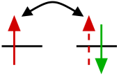
Figure 2: The second-order virtual exchange process in the Hubbard model which leads to the antiferromagnetic Heisenberg coupling, see Ref. Auerbach (1994).

Several variations of this model are known. For example, when $J^{xy}=0$, it is termed Heisenberg model with an Ising anisotropy, or, more generally, with XY anisotropy, if $J^{z}\neq J^{xy}$. Additional terms such as $H^{n}_{j}=D(S^{z}_{j})^{2}$ (“single-ion anisotropy”), or a biquadratic coupling, $H^{bq}_{jm}=J_{2}\;\left({\bf S}_{j}\cdot{\bf S}_{m}\right)^{2}$ can be introduced. When doped below half-filling, the strong-coupling limit of the Hubbard model is described by the $t$–$J$ model

$$H^{tJ}=\mathcal{P}\;H^{tb}\;\mathcal{P}+J\;\sum\limits_{\langle j,m\rangle}\left({\bf S}_{j}\cdot{\bf S}_{m}\;-\;\frac{1}{4}n_{j}\;n_{m}\right),$$ (11)

where $\mathcal{P}$ projects onto the space of singly occupied sites, see, e.g., Ref. Auerbach (1994), leading to a site-basis with three states per site. This Hamiltonian on a two-dimensional square lattice has been proposed as an effective model for the CuO₂ planes in the high-$T_{c}$ superconductors.

A third important class of models are Hamiltonians describing systems containing impurities. A prominent example is the Anderson impurity model, which models the hybridization of the localized $d$ (or $f$) orbital of an impurity located at a site $j$ with conduction-band orbitals (in the simplest case) located at that site, while the electrons on the impurity interact with each other via a Hubbard term. The localized part of the Hamiltonian is then

$$H^{AI}_{j}\;=\;\sum\limits_{\sigma}\varepsilon_{d}\,n^{d}_{j,\sigma}\;+\;V\sum\limits_{\sigma}\left(d^{\dagger}_{j,\sigma}\,c^{\phantom{\dagger}}_{j,\sigma}+{\rm H.c.}\right)\;+\;Un^{d}_{j,\uparrow}n^{d}_{j,\downarrow}\;,$$ (12)

while the conduction band is modeled as a tight-binding band (6). Here $d^{(\dagger)}_{j,\sigma}$ is the annihilation (creation) operator for a fermion with spin $\sigma$ on the impurity site, and $n^{d}_{j,\sigma}=d_{j,\sigma}^{\dagger}d_{j,\sigma}$. This problem has been treated with one or two impurities, leading to the the single or two impurity Anderson model, (SIAM or TIAM, respectively) or as a system with impurities located at every lattice site, leading to the periodic Anderson model (PAM).

Perhaps the most well-known example of an impurity system is the Kondo model, which describes the localized impurity level as a quantum mechanical spin ${\bf S}$, leading to the on-site Hamiltonian

$$H^{K}_{j}=\frac{J_{K}}{2}\;{\bf S}_{j}\cdot\left(c^{\dagger}_{j,\alpha}\sigma^{\phantom{{\dagger}}}_{\alpha,\beta}c^{\phantom{{\dagger}}}_{j,\beta}\right)$$ (13)

where $\sigma^{\phantom{{\dagger}}}_{\alpha,\beta}$ is a vector whose components are the Pauli matrices. This model can be derived as the limit of the symmetric SIAM at strong coupling, $U\gg(t,V)$ Schrieffer and Wolff (1966).

1.1.2 Lattices

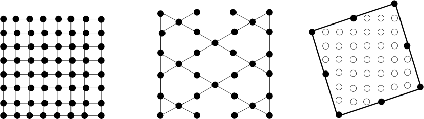
Figure 3: Examples of two-dimensional lattices. On the left and in the middle the square and the Kagomé lattices, respectively, are shown. The sketch on the right shows how a lattice can be tilted along the symmetry axis – in this way, it is possible to treat larger system sizes by exploiting possible additional translation symmetries.

The lattice structure of a regular solid is described by a Bravais lattice, which is built up from a unit cell and a set of translation vectors which create the regular pattern. Since the memory of a computer is finite, it is often necessary to restrict the treatment to finite lattices. In this case, boundary conditions must be specified. For open boundary conditions (OBC, sometimes they are also called fixed BC) the intersite terms of the Hamiltonian are simply set to zero at the boundaries. This leads to a lattice which is not translationally invariant. Translational invariance can be restored on a finite lattice by applying periodic boundary conditions (PBC, also sometimes called Born-von-Kármán BC), in which the edges of the lattice are connected together in a ring geometry for one-dimensional systems or a torus for two-dimensional systems. It is also possible to introduce a phase at the boundaries, leading to antiperiodic or twisted boundary conditions. In Fig. 3 some examples of two-dimensional lattices are shown.

Lattices possess symmetries which can be exploited in calculations. The translation symmetries, parameterized by multiples of the Bravais lattice vector, can be used for boundary conditions that do not break translational invariance, i.e., (A)PBC or twisted boundary conditions. Other useful and simple symmetries are symmetries under a discrete lattice rotation, e.g., rotation by $\pi/2$ for a square lattice (group $C_{4v}$), or reflections about a symmetry axis.

In order to have more sizes available for two-dimensional translationally invariant lattices, it is helpful to work in geometries where the clusters are tilted with respect to some symmetry axis, as depicted in Fig. 3. For the two dimensional square lattices, the spanning vectors for such tilted lattices are given by $F_{1}=(n,m)$, $F_{2}=(-m,n)$ and the total number of sites is then $N=n^{2}+m^{2}$. The lattice periodicity then appears for translations at appropriate values of $(n,m)$. Reflection and discrete rotation symmetries are still present in these lattices, although they become somewhat more complicated. For methods which treat the entire Hilbert space, such as exact diagonalization, it can be important to use these symmetries to reduce as much as possible the dimension of the basis that must be treated numerically.

2 Exact Diagonalization

The expression “Exact Diagonalization” is used to describe a number of different approaches which yield numerically exact results for a finite lattice system by directly diagonalizing the matrix representation of the system’s Hamiltonian in an appropriate many-particle basis. The simplest, and the most time- and memory- consuming approach is the complete diagonalization of the matrix which enables one to calculate all desired properties. However, as shown in the introduction, the dimension of the basis for a strongly interacting quantum system grows exponentially with the system size, so that it is impossible to treat systems with more than a few sites. If only properties of low- or high-lying eigenstates are required, (in the investigation of condensed matter systems one is often interested in the low-energy properties), it is possible to reach substantially larger system sizes using iterative diagonalization procedures, which also yield results to almost machine precision in most cases. The iterative diagonalization methods allow for the calculation of ground state properties and (with some extra effort) some low-lying excited states are also accessible. In addition, it is possible to calculate dynamical properties (e.g., spectral functions, time-evolution) as well as behavior at finite temperature. Nearly every system and observable can be calculated in principle, although the convergence properties may depend on the system under investigation. In the following, we describe the most useful methods and their variants, which should allow for the investigation of most systems of interest.

We also discuss the use of the symmetries of a system, which can be important in reaching the largest possible system sizes, because the dimension of the matrices to be diagonalized is then significantly reduced. An additional advantage is that the results obtained are resolved according to the quantum numbers associated with the symmetries. Useful introductions and discussion of the use of symmetries for specific example Hamiltonians can be found in Refs. Lin (1990); Golinelli et al. (1994); Malvezzi (March 2003). A more general mathematical description in terms of group theory is presented in Ref. Laflorencie and Poilblanc (2004).

With present-day computers, system sizes can be treated which are large enough to provide insight into the physics of many systems of interest. It is possible to treat $S=1/2$ spin models with up to about $N=40$ sites; the maximum sizes reached thus far are, $N=40$ sites on a square lattice, $N=39$ sites on a triangular lattice, and $N=42$ sites on a star lattice geometry. The $t$-$J$ model on a checkerboard and on a square lattice with 2 holes have been treated on up to $N=32$ sites. Hubbard models at half filling on a square lattice with up to $N=20$ sites have been diagonalized; the same size was also reached for quantum dot structures. Models with phonon degrees of freedom such as the Holstein model, are much harder to treat because the phonons are bosons, which, in principle, have an infinite number of degrees of freedom. By truncating the number of phonon states, it was possible to treat a chain with $N=14$ + phonon pseudo-sites. For these calculations, it was necessary to store between $1.5-30\cdot 10^{9}$ basis states Läuchli (talk given at the first ALPS users’ workshop in Lugano, Sept. 2004).

2.1 Representation of Many Body States

In order to represent the many-body basis on a computer, it is convenient to map the states of the site basis to a single bit or to a set of bits. Thus, every basis state $|\alpha^{(\ell)}_{1},\alpha^{(\ell)}_{2},\ldots\alpha^{(\ell)}_{N}\rangle$ can be mapped to a sequence of bits. In C or C++, the most efficient way to handle a bit sequence is to work directly on the bit representation of a (long) unsigned integer variable using bit-operators.

There is usually a natural bit representation for a particular choice of the site basis, The terms of the Hamiltonian then can be implemented as sequences of bit operations on the chosen bit set. For example, a basis state of a Heisenberg spin-1/2 lattice may be mapped to the bit sequence

$$|\uparrow_{1}\downarrow_{2}\downarrow_{3}\ldots\uparrow_{N-1}\uparrow_{N}\rangle\longrightarrow 1_{1}0_{2}0_{3}\ldots 1_{N-1}1_{N}\;.$$

In C or C++, a spin flip operation can be implemented compactly and efficiently as a sequence of boolean operations that invert a particular bit.

For Hubbard-like models, one natural choice for the site basis to the mapping is

$$|N_{l}^{\uparrow}N_{l}^{\downarrow}\rangle\longrightarrow N_{l}^{\uparrow}N_{l}^{\downarrow}$$

with $N_{l}^{\sigma}=\{0,1\}$, i.e., one needs two bits for the mapping of a single site. Alternately, a mapping $|N_{l}^{e}S_{l}^{z}\rangle\longrightarrow N_{l}^{e}S_{l}^{z}$ may also be used (mapping $S^{z}_{\ell}=\{\pm 1/2\}$ to the bits $\{0,1\}$).

Other models can be implemented similarly; for bosonic systems, however, it is necessary to introduce a cut-off in the number of particles per site so that the site basis has a finite number of states. Typically, one only keeps a very small number of on-site bosons, which may depend on the desired system sizes and the parameter values. A minor complication occurs when the number of bits needed to represent a state exceeds the number of bits in an integer; then more than one integer variable must be used for the description of a single basis state.

In order to minimize the dimension of the Hamiltonian matrix, it is essential to exploit symmetries of the system, as described in more detail in Ref. Laflorencie and Poilblanc (2004). Given a symmetry group $\mathcal{G}$ with generators $g_{p}$, if

$$[H,g_{p}]=0,$$ (14)

the Hilbert space can be partitioned into sectors corresponding to irreducible representations of the symmetry group so that the Hamiltonian matrix $\mathbf{H}$ becomes block diagonal. The solution of the eigenvalue problem for each block then yields the portion of the spectrum of the system associated with a particular conserved quantum number.

It is possible to exploit continuous symmetries, such as the conservation of the particle number or the conservation or the $z$ projection of the spin, $S^{z}$. For these Abelian U(1)-symmetries, the conserved quantum numbers correspond to the sum of all bits representing a basis state. Therefore, all possible basis states preserving this symmetry can be obtained by calculating all possible permutations of the bits representing a suitable basis state. Another important symmetry is the conservation of the total spin, which is an SU(2) symmetry. This symmetry is more difficult to implement than U(1) symmetries because it is non-Abelian. However, the $Z_{2}$ symmetry corresponding to spin inversion can be used instead and is easily implemented. Space group symmetries include translational invariance, which is an Abelian symmetry, or point group symmetries such as reflections or rotations, which are non-Abelian in general. A set of representative basis states can be formed from symmetrized linear combinations of the original basis states generated by applying the appropriate generators Laflorencie and Poilblanc (2004).

As an example of how symmetries can reduce the dimension of the largest block of the Hamiltonian that must be diagonalized, we show the size of the sector containing the ground state in Table 1 for a $S=$1/2 Heisenberg model on a $\sqrt{40}\times\sqrt{40}$ cluster. In this case, the dimension of the sector to be diagonalized is reduced by a factor of more than 2500.

full Hilbert space:	dim$=2^{40}=10^{12}$
constrain to $S_{z}=0$:	dim$=138\times 10^{9}$
using spin inversion:	dim$=69\times 10^{9}$
utilizing all 40 translations:	dim$=1.7\times 10^{9}$
using all 4 rotations:	dim$=430,909,650$

Table 1: The reduction of the dimension of the sector of the Hamiltonian containing the ground state for the $S=1/2$ Heisenberg model on a tilted square lattice with $\sqrt{40}\times\sqrt{40}$ sites (from Ref. Läuchli (talk given at the first ALPS users’ workshop in Lugano, Sept. 2004)).

After considering the symmetries, a set of basis states $\{|n\rangle\}$ is stored in an appropriate form such as a set of bit strings or linear combinations of bit strings. The multiplication is then carried out as

$$H|\psi\rangle=\sum_{n}\langle n|\psi\rangle H|n\rangle$$ (15)

where the set of coefficients $\langle n|\psi\rangle$ is a stored as vector of real (or complex) numbers with dimension equal to that of the targeted block of $H$. When the Hamiltonian is applied to a basis state $|n\rangle$, the result is a linear combination of basis states

$$H|n\rangle=\sum_{n^{\prime}}\langle n^{\prime}|H|n\rangle|n^{\prime}\rangle\;,$$ (16)

where there are typically only few nonzero terms for a short-ranged Hamiltonian. When the states $|n\rangle$ can be represented as bit strings, it is usually easy to identify the bit string corresponding to the $\{|n^{\prime}\rangle\}$ and to determine the coefficients $\langle n^{\prime}|H|n\rangle$. However, the bit strings then have to be mapped back to an index into the vector of basis coefficients in order to calculate the coefficients $\langle n|\psi\rangle$. A simple way to implement the needed bookkeeping is to index all the basis states $|n\rangle$ by an integer corresponding to the bit string and to store this index in an additional vector. In this way, it is easy to identify which element of the coefficient vector has to be modified. This implementation is simple and fast, but the index vector is of the dimension of the full bit string used to encode the states and is thus not memory efficient. More memory-efficient implementations are possible; for example, the bit strings could be stored in a lookup-table along with the associated indices and the lookup could be performed using a hash table Press et al. (1993).

2.2 Complete Diagonalization

The diagonalization of real symmetric or complex Hermitian matrices is a problem often encountered in numerical methods in physics. For example, as we will see later, in one step of the DMRG procedure it is necessary to diagonalize the density matrix, represented as a dense, real, symmetric matrix. A number of software libraries provide complete diagonalization routines which take a matrix as input and return all of the eigenvalues and eigenvectors as output. Among the most prominent are the NAG librarynag (NAG, commercial library), the routines published in Numerical Recipes Press et al. (1993); Quarteroni et al. (2000) as well as the LAPACK lap (LAPACK, Fortran and C libraries; an implementation of the BLAS library is required for this package) library, which in combination with the BLAS bla (BLAS, Fortran libraries providing basic matrix and vector operations); atl (ATLAS, efficient BLAS library, needs to be compiled); lib (we find this implementation of the BLAS to be the fastest) provides a very efficient non-commercial implementation of linear algebra tools. Such routines could, in principle, also be used to diagonalize the Hamiltonian matrix of a finite quantum lattice system directly. However, they are, in general, substantially less efficient than the iterative methods described in Sec. 2.3 for finding the low-lying states of the sparse matrices found for such systems.

The approach normally used Press et al. (1993) is first to transform the matrix to tridiagonal form using a sequence of Householder transformations and then to diagonalize the resulting tridiagonal matrix $\mathbf{T}$ using the QL or QR algorithm, which carries out a factorization $\mathbf{T}=\mathbf{QL}$ with $\mathbf{Q}$ an orthogonal and $\mathbf{L}$ a lower triangular matrix. The computational cost of this combined approach scales as $\frac{2}{3}n^{3}$ if only the eigenvalues are obtained, and $\approx 3n^{3}$ when the eigenvectors are also calculated, where $n$ is the dimension of the matrix.

The limitations of using such complete diagonalization algorithms to diagonalize the Hamiltonian matrix are obvious: the entire matrix has to be stored and diagonalized. Since the dimension of the Hamiltonian matrix grows exponentially with system size even when all symmetries are taken into account, the largest attainable lattice sizes for strongly correlated quantum systems are generally very small. For a Hubbard chain, one may reach less than 10 sites on a supercomputer, while with the iterative diagonalization procedures (presented in Sec. 2.3) around 20 sites can be reached when most of the symmetries of the system are taken into account. As we will see later, one-dimensional systems containing more than 1000 sites can be treated on a standard desktop PC using the DMRG, a method carrying out an iterative diagonalization in a reduced Hilbert space. A complete diagonalization of the Hamiltonian matrix is nevertheless useful for testing purposes, and if a significant fraction of all eigenstates is needed on small systems.

2.3 Iterative Diagonalization: the Lanczos and the Davidson Algorithm

If only the ground state and the low-lying excited states of a system are required, powerful iterative diagonalization procedures exist which can handle matrix representations of the Hamiltonian with a dimension substantially (up to four or five orders of magnitude for short-range quantum lattice models) larger than complete diagonalization. These methods can be extended to investigate dynamical properties, time evolution, and the finite-temperature behavior of the system. In addition, they form a key part of the DMRG algorithm, which carries out an iterative diagonalization in an optimal, self-consistently generated reduced basis for a system.

The basic common idea of the different iterative diagonalization algorithms is to project the matrix to be treated $H$ onto a subspace of dimension $M\ll N$ (where $N$ is the dimension of the Hilbert space in which the diagonalization is carried out) which is cleverly chosen so that the extremal eigenstates within the subspace converge very quickly with $M$ to the extremal eigenstates of the system. The main approach used in physics is the Lanczos method, while in quantum-chemistry the Davidson or its generalization the Jacobi-Davidson algorithm is more widely used.

A number of standard textbooks treat numerical methods for matrix computations in detail. In this section, we will discuss only the basic Lanczos and Davidson methods for handling hermitian eigenvalue problems for pedagogical reasons. For further details and for the applicability of the methods to non-hermitian and to generalized eigenvalue problems, we refer the reader to the following sources: Refs. Parlett (1980); Golub and Loan (1996); Watkins (2002) discuss numerical methods for matrix computations in general and also include iterative diagonalization algorithms, including the more modern Jacobi-Davidson algorithm (at least in the later editions). A nice overview and a compact representation of the algorithms can be found in Ref. Bai et al. (2000). The mathematical theory of the Lanczos algorithm has been worked out in Ref. Cullum and Willoughby (1985).

The basic idea behind iterative diagonalization procedures is illustrated by the very simple power method. In this approach, the eigenpair with the extremal eigenvalue is obtained by repeatedly applying the Hamiltonian to a random initial state $|v_{0}\rangle$,

$$|v_{n}\rangle=H^{n}|v_{0}\rangle\;.$$ (17)

Expanding in the eigenbasis $H|i\rangle=\lambda_{i}|i\rangle$ yields

$$|v_{n}\rangle = \sum\limits_{i}\,\langle i|v_{0}\rangle\,H^{n}|i\rangle$$

$$= \sum\limits_{i}\,\langle i|v_{0}\rangle\,\lambda_{i}^{n}|i\rangle\;.$$

It is clear that the state with the eigenvalue with the largest absolute value will have the highest weight after many iterations $n$, provided that $|v_{0}\rangle$ has a finite overlap with this state. The convergence behavior is determined by the spacing between the extremal eigenvalue and the next one; the contribution of the state with the eigenvalue with the next-highest magnitude will not be negligible if the difference between the magnitudes of these eigenenergies is not sufficiently large. Since the convergence of the power method is generally much poorer than other methods we will discuss below, it is generally not used in practice. However, the approach is very simple to implement and is very memory efficient because only the two vectors $|v_{n}\rangle$ and $|v_{n-1}\rangle$ must be stored in memory.

The subspace generated by the sequence of steps in the power method,

$$\{|v_{0}\rangle,H|v_{0}\rangle,H^{2}|v_{0}\rangle,...,H^{n}|v_{0}\rangle\}$$ (18)

is called the $n^{\rm th}$ Krylov space and is the starting point for the other procedures.

2.3.1 The Lanczos Method

In the Lanczos method Lanczos (1950), the Hamiltonian is projected onto the Krylov subspace using a basis generated by orthonormalizing the sequence of vectors (18) to each other as they are generated. This results in a basis in which the matrix representation of the Hamiltonian becomes tridiagonal. The basic algorithm is as follows:

• Choose an initial state $|u_{0}\rangle$ which can be represented in the system’s many-body basis $|n\rangle$, and which has finite overlap with the groundstate of the Hamiltonian. This can be done by taking $\{|n\rangle\}$ as a vector with random entries.

• Generate the states of the Lanczos basis using the recursion relation

  $$|u_{n+1}\rangle = H\;|u_{n}\rangle-a_{n}|u_{n}\rangle-b_{n}^{2}\;|u_{n-1}\rangle$$

  $$\mbox{where}\quad a_{n} = \frac{\langle u_{n}|H|u_{n}\rangle}{\langle u_{n}|u_{n}\rangle}$$

  $$\mbox{and}\quad b_{n}^{2} = \frac{\langle u_{n}|u_{n}\rangle}{\langle u_{n-1}|u_{n-1}\rangle}$$ (19)

  with $b_{0}\equiv 0$ and $|u_{-1}\rangle\equiv 0$. Note that the Lanczos vectors in this formulation of the recursion are not normalized.

• Check if the stopping criterion $\langle u_{n+1}|u_{n+1}\rangle<\varepsilon$ is fulfilled.
  If yes: carry out step 4) and then halt.
  If no: continue.

• Repeat starting with 1) until $n=M$ (the maximum dimension).

• If the stopping criterion is fulfilled, diagonalize the resulting tridiagonal matrix

  $$\mathbf{T}_{n}=\left(\begin{array}[]{ccccc}a_{0}&b_{1}&&&\\ b_{1}&a_{1}&b_{2}&\mathbf{0}&\\ &b_{2}&a_{2}&\ddots&\\ &\mathbf{0}&\ddots&\ddots&b_{n}\\ &&&b_{n}&a_{n}\\ \end{array}\right)$$ (20)

  using the QL algorithm. Note that the off-diagonal elements have the value $b_{i}$ and not $b_{i}^{2}$ for normalized Lanczos vectors $|u_{i}\rangle$. The diagonalization yields eigenvalues $E_{0},\,\ldots,\,E_{n}$, and eigenstates $|\psi_{0}\rangle,\,\ldots,\,|\psi_{n}\rangle$ which are represented in the Lanczos basis.

• In order to avoid storing all of the basis states $|u_{0}\rangle,\ldots,|u_{n}\rangle$, the procedure can be repeated (starting with the same initial vector $|u_{0}\rangle$) to calculate the eigenstates represented in the original many-body basis. This is necessary in order to be able to calculate properties dependent on the wavefunction, such as quantum mechanical observables. One obtains the coefficients $\alpha_{n}$ of the eigenstate in the original many-body basis $|n\rangle$ by carrying out the basis transformation

  $$|\psi_{m}\rangle = \sum\limits_{i}c_{i}\,|u_{i}\rangle$$ (21)

  $$= \sum\limits_{n}\sum\limits_{i}c_{i}\,\langle n|u_{i}\rangle|n\rangle\;,$$

  with $\alpha_{n}\equiv\sum\limits_{i}c_{i}\,\langle n|u_{i}\rangle$.

The algorithm is memory efficient, since only the 3 vectors $|u_{n-1}\rangle,\,|u_{n}\rangle$, and $|u_{n+1}\rangle$ need to be stored at once. Note that it is also possible to formulate the algorithm in a way such that only 2 vectors need to be stored at the cost of complicating the algorithm moderately; the memory efficiency is then the same as the power method. As is typically the case in iterative diagonalization procedures, the most time-consuming step is carrying out the multiplication $H|u_{n}\rangle$, which should be implemented as efficiently as possible, either as described in Sec. 2.1, or using other sparse-matrix multiplication routines. The time needed to perform the other steps of the algorithm is generally negligible when $N$ is realistically large. Therefore, optimizing the routine performing $H|\psi\rangle$ is crucial to the efficiency of the implementation.

The Lanczos procedure results in a variational approximation to the extremal eigenvalue which usually attains quite high accuracy after a number of iterations much smaller than the dimension of the Hilbert space. Typically, 100 recursion steps or less are sufficient to attain convergence to almost machine precision for ground state properties Dagotto (1994). As is evident because the Lanczos method is based on the power method, convergence to extremal eigenvalues occurs first; additional iterations are then necessary to obtain converged excited states. The algorithm is generally considered to be a standard method which can be robustly applied to a wide spectrum of systems. Nevertheless, there are two technical problems which require some care to be taken. First, the convergence of excited states can be irregular; in particular apparent convergence to a particular value can occur for some range of iterative steps, followed by a relatively abrupt change to another, substantionally lower value. It is therefore important to carry out sufficient iterations for the higher excited states. Generally, the number of iterations required to obtain convergence becomes larger for higher excited states.

The second technical problem is the appearance of so-called “ghost” eigenvalues, i.e., spurious eigenvalues which cannot be mapped to eigenvalues of the original Hamiltonian. The origin of such “ghost” eigenvalues can be traced to the loss of the orthogonality of the Lanczos vectors $|u_{n}\rangle$ due to finite machine precision. This is an intrinsic limitation of the algorithm. For this reason, the much more stable Householder algorithm Press et al. (1993) rather than the Lanczos procedure is generally used to transform an entire matrix to tridiagonal form. However, because of the good convergence to the ground state and the algorithm’s memory efficiency, the Lanczos method is nevertheless widely used for the investigation of quantum lattice systems with short-ranged coupling.

With some extra effort, it is also possible to overcome the loss of orthogonality which is a basic drawback of the algorithm. The most straightforward solution is to reorthogonalize the Lanczos vectors relative to each other using a modified Gram-Schmidt procedure. However, this requires all vectors $|u_{n}\rangle$ to be stored in memory, so that the advantage of memory efficiency is lost. However, an appropriately chosen partial reorthogonalization is also sufficient; for details see Ref. Golub and Loan (1996); Watkins (2002); Bai et al. (2000). Cullum and Willoughby Cullum and Willoughby (1985, 1981) developed a method to eliminate ghost states without reorthogonalizing the Lanczos vectors. In their approach, the eigenvalues of the resulting tridiagonal matrix $\mathbf{T}_{n}$ are compared to the ones of a similar matrix $\tilde{\mathbf{T}}_{n}$, which can be obtained by deleting the first row and column of $\mathbf{T}_{n}$. This gives a heuristic criterion for the elimination of spurious eigenvalues: since the ghost eigenvalues are generated by roundoff errors, they do not depend on the initial state $|v_{0}\rangle$ and will be the same for both matrices. After sufficiently many iterations, ghost eigenvalues will converge towards true eigenvalues of the original matrix $\mathbf{H}$. Thus, every multiple eigenvalue of $\mathbf{T}_{n}$ is not a ghost and every unique eigenvalue which is not an eigenvalue of $\tilde{\mathbf{T}}_{n}$ is a true eigenvalue of $H$. This approach is as memory-efficient as the original Lanczos algorithm and approximately as fast, but generally yields the wrong multiplicity for the eigenvalues.

A variant of the algorithm which is easy to implement is the “modified” Lanczos method Dagotto (1994). In this approach, the recursion procedure is terminated after two steps, i.e., only two Lanczos vectors are considered and the resulting $2\times 2$ matrix is diagonalized. The resultant eigenvector is taken as the starting point for a new $2\times 2$ Lanzcos procedure; this process is then repeated until convergence (i.e., the change in $|\lambda_{0}|$ is sufficiently small) is achieved. The modified Lanczos method has only limited usefulness: the convergence is only marginally better than the power method and excited states are rather difficult to obtain. However, the idea of restarting the Lanczos procedure is often used in practical implementations, i.e., after $\sim 10$ to $\sim 100$ Lanczos iterations, the resulting tridiagonal matrix is diagonalized and the extremal eigenstate is used as starting vector for a new Lanczos procedure. Further important variants of the algorithm are the implicitly restarted Lanczos method and the Band- or Block-Lanczos method. The latter puts the “modified” Lanczos variant on a more systematic footing and deals with the problem that it is not a priori known how many iterations are needed for convergence by limiting the number of steps and then restarting the Lanczos-procedure with an appropriate, better initial vector obtained by taking into account the outcome of the previous Lanczos run. The Block Lanczos approach is useful when degeneracies are present in the desired eigenvalues and all eigenstates and eigenvalues of the corresponding subspace must be obtained. Rather than starting with a single initial state vector $|u_{0}\rangle$, a set of $p$ orthonormal state vectors $|u_{0}^{(1)}\rangle,|u_{0}^{(2)}\rangle,\ldots,|u_{0}^{(p)}\rangle$ is used to initialize the Lanczos procedure. For an eigenstate with degeneracy $g_{d}$, $p\geq g_{d}$ should be chosen in order to fully resolve the degenerate subspace. The Lanczos procedure is then performed on this subspace and a block-tridiagonal matrix is obtained. For details and for other variants of the Lanczos procedure, see e.g., Ref. Bai et al. (2000).

Figure 4: Typical convergence behavior of the Lanczos algorithm. In this example, convergence to the ground-state is already reached after approximately 10 iterations, while additional iterations are required to reach convergence for the excited states. “Ghost” eigenvalues appear and converge to a real eigenvalue as additional iterations are performed, leading to erroneous multiplicity at the completion of the calculation.

The generalization of the Lanczos method to non-hermitian operators is the Arnoldi method, see, e.g., Ref. Bai et al. (2000). For such problems, a Krylov-space approach similar to the Lanczos procedure is used to reduce a general matrix to upper Hessenberg form.

A number of software packages are available which provide implementations of iterative diagonalization routines, such as ARPACK arp (ARPACK, a collection of Fortran subroutines) or the IETL iet (IETL, provides generic C++ routines), a part of the ALPS-library alp (ALPS, see cond-mat/0410407). In order to use this software, a routine which performs the multiplication $H|\psi\rangle$ must be defined by the user; an effient implementation is crucial to the overall efficiency of the algorithm.

There have been many investigations using the Lanczos procedure. Examples for recent work using ED are investigations treating frustrated quantum magnets, Ref. Lauchli and Poilblanc (2004), two-leg ladder systems, Ref. Roux et al. (unpublished), transport through molecules and nanodevices Aligia et al. (2004), and atomic gases on optical lattices Damski et al. (unpublished).

2.3.2 Davidson and Jacobi-Davidson

The common idea of iterative diagonalization methods is to project the matrix to be diagonalized onto a subspace much smaller than the complete Hilbert space. The subspace, spanned by a set of orthonormal states $\left\{|u_{k}\rangle\right\}$, is then expanded in a stepwise manner so that the approximation to the extremal eigenstates improves. At particular points in or at the end of the procedure, the representation of the Hamiltonian matrix in this subspace is diagonalized. The resulting extremal eigenvalue $\tilde{\lambda}_{k}$ is called the Ritz-value and the corresponding eigenvector the Ritz-vector $|\tilde{\psi}_{k}\rangle$. According to the Ritz variational principle, $\tilde{\lambda}_{k}$ is always an upper bound to the real ground state energy, see, e.g., Ref. Cohen-Tannoudji et al. (1996). The error in applying $H$ to the eigenvector $|\tilde{\psi}_{k}\rangle$ associated with the Ritz-value $\tilde{\lambda}_{k}$, is approximated by the residual vector

$$|r_{k}\rangle=H|\tilde{\psi}_{k}\rangle-\tilde{\lambda}_{k}|\tilde{\psi}_{k}\rangle\;.$$ (22)

(This expression would be exact if $\tilde{\lambda}_{k}$ were replaced by the exact eigenvalue $\lambda_{k}$.) In the Lanczos procedure, the recursion is formulated so that the subspace is expanded by the component of the residual vector $|r_{k}\rangle$ orthogonal to the subspace.

In 1975, Davidson formulated an alternate iterative algorithm in which the subspace is expanded in the following way Davidson (1975). The exact correction to the Ritz-vector is given by

$$|z\rangle=|\psi\rangle-|\tilde{\psi}_{k}\rangle$$

so that

$$\left(\mathbf{H}-\lambda_{k}\mathbf{1}\right)|z\rangle=-\left(\mathbf{H}-\lambda_{k}\mathbf{1}\right)|\tilde{\psi}_{k}\rangle\;.$$ (23)

Thus, solving

$$\left(\mathbf{H}-\lambda_{k}\mathbf{1}\right)|z\rangle=-|r_{k}\rangle$$ (24)

would lead to the exact correction to $|\tilde{\psi}_{k}\rangle$. This amounts to inverse iteration (see, e.g., Ref. Press et al. (1993)). However, the exact eigenvalue $\lambda_{k}$ is not known, and the numerical solution of this linear system is of comparable numerical difficulty to the entire iterative diagonalization. Davidson’s idea was to approximate the correction vector $|z\rangle$ by

$$|\tilde{z}\rangle=-(\mathbf{D}-\tilde{\lambda}_{k}\mathbf{1})^{-1}|r_{k}\rangle\;,$$ (25)

where the diagonal matrix $\mathbf{D}$ contains the diagonal elements of $\mathbf{H}$. This is a good approximation if $\mathbf{H}$ is diagonally dominant. If $\mathbf{D}$ were replaced by the unit matrix $\mathbf{1}$, the Davidson algorithm would be equivalent to the Block Lanczos procedure. Therefore, if the diagonal elements of $\mathbf{H}$ were all the same, both methods would have the same performance. For many problems, however, this variation of the diagonal elements is important and the Davidson algorithm converges more rapidly.

In its original formulation, the Davidson algorithm follows the procedure Davidson (1975):

• If the $k$th eigenvalue is to be obtained, choose a subspace of $l\geq k$ orthonormal vectors $|v_{1}\rangle,\,|v_{2}\rangle,\,\ldots,\,|v_{l}\rangle$. In the following, the matrix $\mathbf{B}$ is the matrix containing these vectors as columns.

• • Form and save the vectors $H|v_{1}\rangle,\,H|v_{2}\rangle,\,\ldots,\,H|v_{l}\rangle$. In the following, the matrix $\mathbf{\tilde{A}}$ is the matrix containing these vectors as columns.

  • Construct the matrix $\mathbf{A}=\langle v_{i}|H|v_{j}\rangle$ and diagonalize it, obtaining the $k$th eigenvalue $\lambda_{k}^{(l)}$ and the corresponding eigenvector $|\alpha_{k}^{(l)}\rangle$. The upper index $(l)$ denotes that this eigenpair was obtained by keeping $l$ vectors for building the matrix $\mathbf{A}$.

• Form the residual vector corresponding to the $k$th eigenvector,

  $$|q_{l}\rangle=\left(\mathbf{\tilde{A}}-\lambda_{k}^{(l)}\mathbf{B}\right)|\alpha_{k}^{(l)}\rangle.$$

• Calculate the norm $|\,|q_{l}\rangle\,|$. If $|\,|q_{l}\rangle\,|<\epsilon$, accept this eigenpair, otherwise continue.

• Compute the correction vector $|w_{l}\rangle=(\mathbf{D}-\lambda_{k}\mathbf{I})^{-1}|q_{l}\rangle$, where $\mathbf{D}$ is a matrix containing the diagonal elements of $\mathbf{A}$ and $\mathbf{I}$ is the unit matrix. Orthonormalize $|w_{l}\rangle$ against $|v_{1}\rangle,\,|v_{2}\rangle,\,\ldots,\,|v_{l}\rangle$ to form $|v_{l+1}\rangle$. Expand the the matrix $B$ by adding $|v_{l+1}\rangle$ as an additional column.

• Form and save the vector $H|v_{l+1}\rangle$. Set $l=l+1$ and continue with step 1).

Although the Davidson algorithm is somewhat more complicated to implement than the Lanczos algorithm, its convergence is usually higher order than the Lanczos method and it is more stable. In particular, spurious ghost eigenvalues do not appear. The disadvantages compared to Lanczos are that $\langle u_{i}|H|u_{j}\rangle$ is not tridiagonal, and all the $|u_{i}\rangle$ must be kept in order to carry out the explicit orthogonalization in step 4). Similarly to the Lanczos-method, this algorithm can fail for particular choices of the initial vector, e.g., if $|u_{0}\rangle=|\psi_{0}\rangle$. In practice, one performs a small number of Davidson iterations and, if necessary, restarts the procedure using the outcome of the previous iteration as initial vectors $|v_{1}\rangle,\,\ldots,\,|v_{l}\rangle$.

A generalization of the original Davidson approach is given by the Jacobi-Davidson method Sleijpen and van der Vorst (1996). In this approach, one approximates the correction vector $|z\rangle$ by

$$\left(\mathcal{H}-\tilde{\lambda}_{k}\mathbf{1}\right)|\tilde{z}\rangle=-|r_{k}\rangle-\varepsilon|u_{k}\rangle\;,$$ (26)

where $\varepsilon$ is chosen so that that $\langle u_{k}|\tilde{z}\rangle=0$. Here the preconditioner $\mathcal{H}$ is an easily invertible approximation to $\mathbf{H}$. The choice of an optimal preconditioner is non-trivial and must be tailored to suit the specific problem treated. The Jacobi-Davidson method is more general and flexible than the Davidson method and does not suffer from the lack of convergence when $|u_{0}\rangle=|\psi_{0}\rangle$. It is (almost) equivalent to the Davidson method when $\mathcal{H}=\mathbf{D}$. Therefore, it is now widely used instead of the Davidson algorithm, especially in quantum chemistry.

An additional advantage of the Jacobi-Davidson algorithm over the Davidson procedure is that it can be applied to generalized eigenvalue problems,

$$A\;|x\rangle=\lambda\;B\;|x\rangle,$$ (27)

where $A$, $B$ are general, complex $n\times n$ matrices Sleijpen and van der Vorst (1996).

Using these iterative diagonalization algorithms, many different quantum many-body systems can be treated. However, the methods outlined thus far are primarily useful for calculating properties of the ground-state (highest state) and low-lying excited states. Many experimentally interesting properties, such as dynamical correlation functions and other frequency-dependent quantities, or finite-temperature properties cannot be directly calculated from the ground state and low-lying excited states. Nevertheless, methods based on iterative diagonalization have been developed to calculate such properties; these extensions to iterative diagonalization will be discussed in the remainder of this section.

2.4 Investigation of Dynamical Properties

Dynamical quantities in general involve excitations at a particular frequency $\omega$ and are often additionally resolved at momentum $\mathbf{q}$. It is clear that extensions to exact diagonalization must generate a set of states that are appropriate to describe these energy and momentum scales. This can be done by starting with the ground state obtained by a converged iterative diagonalization procedure and applying an appropriate operator or sequence of operators.

Frequency-dependent quantities can be defined as the Fourier transform of time-dependent correlation functions

$$C(t)=-i\langle\psi_{0}|A(t)\;A^{\dagger}(0)|\psi_{0}\rangle\;,$$ (28)

where the operator $A$ generates the desired correlations. The Fourier transform to frequency space then yields ($\omega\geq 0$)

$$\tilde{C}(\omega+i\eta)=\langle\psi_{0}|\,A\,\left(\omega+i\eta-H+E_{0}\right)^{-1}\,A^{\dagger}\,|\psi_{0}\rangle\;,$$ (29)

where the inverse operator in the center is termed the resolvent operator. The spectral function then is given by Mahan (2000)

$$I(\omega)=-\frac{1}{\pi}\lim_{\eta\to 0^{+}}{\rm Im}\,\tilde{C}(\omega+i\eta)\;.$$ (30)

Dynamical quantities can be probed in scattering experiments such as photoemission or neutron-scattering. Examples of choices of $A$ for some typical spectral functions are displayed in Table 2.

name	notation	operators	experiment
single-particle spectral weight	$A({\bf k},\omega)$	$A=c^{\phantom{\dagger}}_{{\bf k},\sigma}$	photoemission
structure factor	$S_{zz}({\bf q},\omega)$	$A=S^{z}_{\bf q}$	neutron scattering
optical conductivity	$\sigma_{xx}(\omega)$	$A=j_{x}$	optics
4-spin correlation	$R(\omega)$	$A=\sum_{\bf k}R_{\bf k}\,{\bf S}_{\bf k}\cdot{\bf S}_{\bf-k}$	Raman scattering

Table 2:

A spectral function can also be expressed in the Lehmann representation

$$I(\omega)=\sum_{n}\;|\langle\psi_{n}|A^{\dagger}|\psi_{0}\rangle|^{2}\;\delta(\omega-E_{n}+E_{0})\;,$$ (31)

which involves a sum over the complete eigenspectrum of the system. Thus, the numerical method must provide the poles $E_{n}$ and the weights $\langle\psi_{n}|A^{\dagger}|\psi_{0}\rangle$ for each eigenstate. While it is possible to calculate the spectral function using this formulation in principle, it is generally prohibitive to calculate the entire eigenspectrum of the system; this amounts to a complete diagonalization of the Hamiltonian.

An alternative approach is to apply Eq. (30) directly. In this case, the resolvent operator must either be calculated directly or approximated.

2.4.1 Krylov Space (or Continued Fraction) Method

Within the Lanczos method, it is convenient to represent operators in a Krylov basis. The frequency-dependent correlation function (29) can be expanded in such a basis if a Lanczos procedure is carried out starting with the initial vector

$$|u_{0}\rangle=\frac{1}{\sqrt{\langle\psi_{0}|\,A\;A^{\dagger}\,|\psi_{0}\rangle}}\,A^{\dagger}\,|\psi_{0}\rangle\;.$$ (32)

Within the Lanzcos basis generated by $H|u_{0}\rangle$, $H^{2}|u_{0}\rangle,\,\ldots\,$, the resolvent operator can be expressed in terms of the Lanczos coefficients $a_{n}$ and $b_{n}$ as a continued fraction Dagotto (1994). The correlation function then has the form

$$\tilde{C}(z=\omega+i\eta+E_{0})=\frac{\langle\psi_{0}|\,A\;A^{\dagger}\,|\psi_{0}\rangle}{z-a_{1}-\frac{b_{2}^{2}}{z-a_{2}-\ldots}}\;.$$ (33)

Therefore, each set of Lanczos coefficients $a_{n}$, $b_{n}$ generates an additional pole of the frequency-dependent correlation function. In practice, the procedure is truncated after a number of poles appropriate to the size of the system and required resolution of the spectral function has been obtained. The weight of each pole typically decreases rapidly with number of steps $n$ so that a moderate number of iterations is usually sufficient in order to obtain the desired quantities.

The low energy part of the spectrum can also be obtained by directly using the Lehmann representation of the spectral function Eq. (31). Truncation after a finite number of terms yields a finite number of poles. However, a fairly large number of eigenstates would have to be calculated directly, which is awkward within iterative diagonalization. Additionally, it is not clear that the weight of each subsequent term would dimish sufficiently rapidly to justify a truncation after only a small proportion of the eigenstates are obtained. The resulting spectral function using this approach is a series of sharp delta peaks located at the poles. In order to obtain a continuous spectrum and to be able to compare to experimental data, it is necessary to introduce a broadening of the peaks by calculating the convolution, e.g., with a Lorentzian.

Note that the appearance of ghost-eigenvalues is not a problem in the calculation of the spectral functions, since the matrix elements associated with the ghost eigenvalues are negligibly small mai (private communication by Andreas Läuchli and Matthias Troyer). This turns out to be true when using the Lehmann-representation as well as when applying the continued fraction approach.

2.4.2 Correction Vector Method

An alternative approach, suggested by Soos and Ramasesha Soos and Ramasesha (1989), is to apply the resolvent operator directly. The vectors

$$|\phi_{0}\rangle=A^{\dagger}\,|\psi_{0}\rangle\;,\hskip 56.9055pt|\phi_{1}\rangle=\left(\omega+i\eta-H+E_{0}\right)^{-1}\,|\phi_{0}\rangle,$$ (34)

are calculated directly starting with the ground state $|\psi_{0}\rangle$ obtained using iterative diagonalization. The spectral function is then given by

$$I(\omega)=\frac{1}{\pi}\;{\rm Im}\,\langle\phi_{0}|\phi_{1}\rangle\;.$$ (35)

The correction vector $|\phi_{1}\rangle$ is obtained by solving the linear system

$$\left(\omega+i\eta-H+E_{0}\right)|\phi_{1}\rangle=|\phi_{0}\rangle\;.$$ (36)

One advantage of this approach are that the spectral weight is calculated exactly for a given frequency $\omega$ rather than approximated as in the continued fraction approach. In addition, it is possible to obtain nonlinear spectral functions by computing higher order correction vectors. This scheme is naturally used in conjunction with the Davidson algorithm, in which the correction to the residual vector must be calculated at each step, whereas the Krylov subspace is not easily available.

The disadvantage of this approach is that it generally is more expensive in computer time because the system of equations, Eq. (36), must be solved for each $\omega$ desired.

2.5 Real Time Evolution

The time evolution of a quantum system is governed by the time-dependent Schrödinger equation

$$i\hbar\frac{\partial}{\partial\,t}|\psi(t)\rangle=H|\psi(t)\rangle\;.$$ (37)

Using the Lanczos-vectors, the time evolution through one interval $U_{dt}|\psi\rangle$ can be approximated by Hochbruck and Lubich (1999); Moler and Loan (2003)

$$|\psi(t+dt)\rangle=e^{-idt/\hbar\,H}\,|\psi(t)\rangle\approx\mathbf{V}_{n}(t)\;e^{-idt/\hbar\,\mathbf{T}_{n}(t)}\;\mathbf{V}_{n}^{T}(t)\;|\psi(t)\rangle\;,$$ (38)

where $\mathbf{V}_{n}$ is the matrix containing all the Lánczos vectors $|u_{j}\rangle$. One finds that for a high accuracy only a very small Krylov space is needed; $n\leq 20$ is sufficient. Therefore, the matrices in Eq. (38) are very small, and the time-evolution can be computed efficiently. For details see the authors contribution to this topic in this volume, Ref. Manmana et al. (2005).

Using this approach, it is possible to study a number of different non-equilibrium properties of strongly correlated quantum systems. It can also be used to obtain dynamical properties by computing the Fourier-transform of a time-dependent correlation function directly. As described in Ref. Manmana et al. (2005), it is possible to construct a time-evolution scheme for the DMRG based on this approach.

2.6 Calculations at Finite Temperature using Exact Diagonalization

All approaches presented so far have been formulated for zero temperature. The calculation of finite-temperature properties is a more demanding task because thermodynamic expectation values are given by sums such as

$$\langle A\rangle=\frac{1}{Z}\sum_{n}^{N}\langle n|Ae^{-\beta H}|n\rangle$$

with the partition function

$$Z=\sum_{n}^{N}\langle n|e^{-\beta H}|n\rangle$$ (39)

where $|n\rangle$ is an orthonormal basis. As in the calculation of dynamical properties, it is prohibitively expensive to sum over all $|n\rangle$ due to the large dimension of the basis. This difficulty is circumvented by a stochastic approach (“stochastic sampling of Krylov space”) developed by Jaklič and Prelovšek Jaklič and Prelovšek (2000). Their approach enables the calculation of thermodynamic properties such as the specific heat, the entropy, or the static susceptibilities of a system, as well as its static and dynamic correlation functions. It is therefore a useful tool for comparing to experiments.

The approach is related to the high temperature series expansion, in which expectation values are given by

$$\langle A\rangle = Z^{-1}\sum\limits_{n}\sum\limits_{k=0}^{\infty}\frac{\left(-\beta\right)^{k}}{k!}\langle n|H^{k}A|n\rangle;,$$ (40)

$$Z = \sum\limits_{n}\sum\limits_{k=0}^{\infty}\frac{\left(-\beta\right)^{k}}{k!}\langle n|H^{k}|n\rangle\;.$$ (41)

Expressions such as $\langle n|H^{k}A|n\rangle$ can be evaluated using the Lanczos vectors and eigenvalues resulting from a Lanczos run:

$$\langle n|H^{k}A|n\rangle=\sum\limits_{i=1}^{M}\langle n|\psi_{i}^{M}\rangle\langle\psi_{i}^{M}|A|n\rangle\left(\varepsilon_{i}^{(M)}\right)^{k}\;.$$ (42)

However, the number of vectors needed is still too large. To overcome this, in a second step one introduces a stochastic sampling over different Krylov spaces, i.e., the Lanczos procedure is performed repeatedly for a variety of random initial vectors, and an average is taken over the samples at the end. This finally leads to the expression

$$\langle A\rangle\approx\frac{1}{Z}\sum_{s}\frac{N_{s}}{R}\sum_{r}^{R}\sum_{m}^{M}e^{-\beta\varepsilon^{(r)}_{m}}\langle r|\Psi^{(r)}_{m}\rangle\langle\Psi^{(r)}_{m}|A|r\rangle$$ (43)

where

$$Z\approx\sum_{s}\frac{N_{s}}{R}\sum_{r}^{R}\sum_{m}^{M}e^{-\beta\varepsilon^{(r)}_{m}}\left|\langle r|\Psi^{(r)}_{m}\rangle\right|^{2}\;.$$ (44)

Here $\sum_{s}$ denotes summation over symmetry sectors of dimension $N_{s}$, $\frac{1}{R}\sum^{R}_{r}$ denotes the average over $R$ random starting vectors $|\Psi^{(r)}_{0}\rangle$, and $\sum_{m}$ is over the $m^{\rm th}$ Lanczos propagation of the corresponding random starting vectors $|\Psi^{(r)}_{m}\rangle$.

This approach is useful if convergence with the number of Lanczos propagations $M\ll N_{s}$ and the number of random samples $R\ll N_{s}$ is sufficiently fast. Due to the relation to the high-$T$ expansion, the $T\to\infty$ limit is reproduced correctly. One obtains high- to medium-temperature properties in the thermodynamic limit. For finite systems, the low-temperature limit is reproduced correctly up to the sampling error Jaklič and Prelovšek (2000). Aichhorn et al. Aichhorn et al. (2003) invented an approach which can be used to reduce the sampling errors at low temperature. They use the property that a twofold insertion of a Lanczos basis leads to smaller fluctuations at low $T$. To do this, the expectation value is expressed as

$$\langle A\rangle=\frac{1}{Z}\sum_{n}^{N}\langle n|e^{-\beta H/2}\,A\,e^{-\beta H/2}|n\rangle\;,$$ (45)

and the projection to the Lanczos basis is performed.

This method has been used, e.g., for the investigation of the planar $t-J$ model at finite temperature Jaklič and Prelovšek (1996).

2.7 Discussion: Exact Diagonalization

As we have seen, the exact numerical treatment of quantum many body systems is hindered by a number of significant obstacles. However, it is possible to formulate conceptually straightforward numerically exact methods which allow the treatment of surprisingly large Hamiltonian matrices, especially when symmetries of the Hamiltonian are taken into account. Extensions to the basic method also make it possible to calculate quantities which, in their simplest formulation, require the calculation of the full eigenspectrum of the Hamiltonian, such as dynamical correlation functions, the time evolution and finite temperature properties. Nevertheless, maximum system sizes remain strongly limited because of the exponential growth of the many-body Hilbert space with system size. In the following sections, we discuss additional numerically exact methods which overcome this restriction, especially for one-dimensional systems, albeit with the introduction of additional approximations. These methods are capable of treating much larger systems, containing up to as much as several thousand sites, allowing a reliable extrapolation to the thermodynamic limit to be performed. However, exact diagonalization nevertheless plays the role of a benchmark for other methods because it provides numerically exact results in most cases, and is useful for problems for which the other approaches fail.

3 Numerical Renormalization Group

The numerical renormalization (NRG) was developed by Wilson as a numerical approach to the single-impurity Kondo and Anderson problems, which, in conjunction with various analytic methods, provides an accurate, complete solution of the problems Wilson (1975). The difficulty in these problems lies in the widely varying energy scales that need to be accurately described. For example, Kondo screening occurs at an exponentially small energy scale set by the Kondo temperature. Perturbation theory, while providing a good description at higher temperatures, breaks down at the Kondo temperature.

Here we will be concerned primarily with illustrating the general concepts and features of the method, exploring the conditions under which it works or does not work, and relating it to other methods; in particular, to exact diagonalization and to the DMRG. More complete treatments of the NRG include Refs. Wilson (1975); Hewson (1997); Costi (1999), on which the material presented here is based.

3.1 Anderson and Kondo problems

The single-impurity Anderson model (SIAM) was introduced by Anderson in 1961 to describe a spherically symmetric strongly correlated impurity in an uncorrelated non-magnetic metal Anderson (1961). In lattice form, its Hamiltonian can be written

$$H^{AI}\;=\;\varepsilon_{d}\,\sum_{\sigma}n^{d}_{\sigma}\;+\;Un^{d}_{\uparrow}n^{d}_{\downarrow}\;+\;\sum_{{\bf k},\sigma}\left(V_{{\bf k},d}\,c^{\dagger}_{{\bf k},\sigma}d^{\phantom{\dagger}}_{{\bf k},\sigma}+{\rm H.c.}\right)\;+\;\sum_{{\bf k},\sigma}\varepsilon_{{\bf k}}\,c^{\dagger}_{{\bf k},\sigma}c^{\phantom{\dagger}}_{{\bf k},\sigma}$$ (46)

where the non-degenerate impurity has energy $\varepsilon_{d}$ and $n^{d}_{\sigma}=d^{\dagger}_{\sigma}d^{\phantom{\dagger}}_{\sigma}$ is its number operator and $d^{\dagger}_{\sigma}$ the corresponding creation operator. The Coulomb interaction $U$ is local and takes place only on the impurity, but the hybridization $V_{{\bf k},d}$ in general allows scattering from all momentum states. The hybridization function

$$\Delta(\omega)=\pi\sum_{\bf k}|V_{{\bf k},d}|^{2}\delta(\omega-\varepsilon_{\bf k})\;,$$ (47)

along with the density of states of the conduction band, $\rho(\omega)=\sum_{\bf k}\delta(\omega-\varepsilon_{\bf k})$, determine the behavior of the system. Here we follow the usual treatment and consider only the orbitally symmetric case, i.e., $V_{{\bf k},d}=V_{kd}$ and $\varepsilon_{\bf k}=\varepsilon_{k}$. This corresponds to taking a completely isotropic electron gas, which can be realized only approximately in a real solid. We then need to consider only the s-wave states of the conduction electrons, so that $c_{\bf k,\sigma}$ can be replaced by $c_{k,l=m=0,\sigma}\equiv c_{k,\sigma}$.

A closely related model is the Kondo or s-d exchange model,

$$H^{K}\,=\,J_{K}\,{\bf S}_{d}\cdot{\bf s}_{0}\,+\,\sum_{{\bf k},\sigma}\varepsilon_{{\bf k}}\,c^{\dagger}_{{\bf k},\sigma}c^{\phantom{\dagger}}_{{\bf k},\sigma}$$ (48)

with ${\bf s}_{0}=f^{\dagger}_{0,\sigma}{\vec{\sigma}}_{\sigma\mu}f^{\phantom{\dagger}}_{0,\mu}$ and localized Wannier state generated by $f^{\phantom{\dagger}}_{0,\sigma}=\sum_{k}c^{\phantom{\dagger}}_{k,\sigma}$, in which the electronic impurity is replaced by a localized spin-1/2 described by the spin operator ${\bf S}_{d}$. The Kondo model can be derived as a strong coupling ($U\gg V$) approximation to the SIAM via the Schrieffer-Wolff transformation in the symmetric case ($\varepsilon_{d}=-U/2$) Schrieffer and Wolff (1966), leading to the correspondence $J_{K}=8V^{2}/U$.

In order to bring the SIAM and the Kondo model into a form amenable to numerical treatment, the models are mapped onto a linear chain model using a Lanczos tridiagonalization procedure. For the SIAM with orbital symmetry, the procedure is carried out as follows. The object is to transform the hybridization into a local term. This can be done by defining the localized Wannier state $|0,\sigma\rangle\equiv f^{\dagger}_{0,\sigma}|\psi_{\rm vac}\rangle$ ($|\psi_{\rm vac}\rangle$ designates the vacuum) with

$$f_{0,\sigma}=\frac{1}{V}\sum_{k}V_{kd}c_{k,\sigma}$$ (49)

and the normalization $V\equiv\left(\sum_{k}|V_{kd}|^{2}\right)^{1/2}$. One then transforms the kinetic energy of the conduction band, $H_{c}=\sum_{k}\varepsilon_{k}c^{\dagger}_{k,\sigma}c^{\phantom{\dagger}}_{k,\sigma}$ to the new set of operators, taking it from diagonal to tridiagonal form, by constructing a sequence of orthogonal states generated by applying $H_{c}$:

$$|1\rangle = \frac{1}{\lambda_{0}}\left[H_{c}|0\rangle-|0\rangle\langle 0|H_{c}|0\rangle\right]$$

$$|n+1\rangle = \frac{1}{\lambda_{n}}\left[H_{c}|n\rangle-|n\rangle\langle n|H_{c}|n\rangle-|n-1\rangle\langle n-1|H_{c}|n\rangle\rangle\right]$$ (50)

(where we have dropped the spin index $\sigma$ for compactness). Note that this is a rather unusual analytic application of what is essentially the Lanzcos procedure of Section 2.3.1. The result is that the SIAM is transformed to the form of a semi-infinite tight-binding chain

$$\tilde{H}^{AI}\;=\;\varepsilon_{d}\,n^{d}_{\ell}\; + \;Un^{d}_{\ell,\downarrow}n^{d}_{\ell,\downarrow}\;+\;V\sum_{{\bf k},\sigma}\,\left(f^{\dagger}_{0,\sigma}d^{\phantom{\dagger}}_{\sigma}+{\rm H.c.}\right)$$

$$+ \;\sum_{n=0,\sigma}^{\infty}\left[\epsilon_{n}\,f^{\dagger}_{n,\sigma}f^{\phantom{\dagger}}_{n,\sigma}\,+\,\lambda_{n}\left(f^{\dagger}_{n,\sigma}f^{\phantom{\dagger}}_{n+1,\sigma}+{\rm H.c.}\right)\right]\;,$$ (51)

where, in second quantized notation, the operators $f^{\dagger}_{n,\sigma}$ create an electron in state $|n\rangle$. The Lanczos coefficients, $\lambda_{n}=\langle n+1|H_{c}|n\rangle$ and $\epsilon_{n}=\langle n|H_{c}|n\rangle$, depend on the dispersion $\varepsilon_{k}$ and the hybridization function $\Delta(\omega)$ of the original SIAM, and, in general, can be determined, in the worst case numerically, during the Lanczos procedure. In general, they do not necessarily fall off with $n$, a property which is crucial for the convergence of the NRG procedure, as we will see below. An analogous procedure can be carried out for the Kondo Hamiltonian (48), starting with the local Wannier state $|0,\sigma\rangle$ generated by $f^{\phantom{\dagger}}_{0,\sigma}=\sum_{k}c^{\phantom{\dagger}}_{k,\sigma}$.

In order to ensure that the tridiagonal chain formulations of the SIAM or the Kondo model lead to a convergent NRG procedure, additional approximations must be made. In particular, a logarithmic discretization of the conduction band leads to coefficients that fall off exponentially with $n$. Here, we will discuss the Kondo model for concreteness, but extension to the SIAM is straightforward. In the first step, we take the density of states of the conduction band to be a constant, $D$. As long as there are no divergences at the Fermi level, the low-energy physics should be dominated by the constant part, as can be justified by expanding the dispersion $\varepsilon_{k}$ in a power series about the Fermi vector $k_{F}$ Wilson (1975). (Generalizations can be made for other densities of states.) The next is a logarithmic discretization of the conduction band $[-D<\varepsilon_{k}<D]$ in energy, i.e., a division into intervals $D^{+}=[\Lambda^{-(n+1)},\Lambda^{-n}]$ and $D^{-}=[-\Lambda^{-n},-\Lambda^{-(n+1)}]$ for the positive and negative parts, respectively (see Fig. 5). For each interval, we can expand the electron creation operators in a Fourier series, defining

$$a^{\dagger}_{n,p,\sigma}\equiv\sum_{[k]_{n}}e^{i\omega_{n}pk}c^{\dagger}_{k,\sigma}\;,$$ (52)

where $[k]_{n}$ is the set of momentum points in the interval $\Lambda^{-(n+1)}<k<\Lambda^{-n}$, $p$ is an integer, and $\omega_{n}=2\pi\Lambda^{n+1}/(\Lambda-1)$. For an interval $\Lambda^{-(n+1)}<k<\Lambda^{-n}$ in the negative range, operators $b^{\dagger}_{n,p,\sigma}$ can be defined analogously, It can be shown that the operators $a^{\dagger}_{n,p,\sigma}$, $b^{\dagger}_{n,p,\sigma}$, and their hermitian conjugates obey the usual anticommutation rules for fermions. For $H^{K}$, Eq. (48), the localized state can be expressed as

$$f^{\dagger}_{0,\sigma}=\left(1-\Lambda^{-1}\right)^{1/2}\;\sum_{n}\Lambda^{-n/2}\;\left(a^{\dagger}_{0,p,\sigma}+b^{\dagger}_{0,p,\sigma}\right)$$ (53)

At this point, the approximation is made to neglect all higher terms in the Fourier series, keeping only one electron per logarithmic energy interval, i.e., $a^{\dagger}_{n,0,\sigma}$ and $b^{\dagger}_{n,0,\sigma}$. Since the impurity only couples directly to the localized state, neglecting these states amounts only to neglecting off-diagonal matrix elements, which can be shown to be proportional to $(1-\Lambda^{-1})$. Therefore, the approximation becomes valid in the limit $\Lambda\to 1$; a more detailed analysis of the errors can be found in Ref. Wilson (1975).

Figure 5: logarithmic discretization of the conduction band.

After applying the tridiagonalization procedure outlined above to the logarithmically discretized version of the Hamiltonian $H^{K}$, we arrive at the effective chain Hamiltonian for the Kondo model

$$\tilde{H}^{K}=\tilde{D}\,\sum_{n=0,\sigma}^{\infty}\,\Lambda^{-n/2}\,\left(f^{\dagger}_{n,\sigma}f^{\phantom{\dagger}}_{n+1,\sigma}+{\rm H.c.}\right)\,+\,2J_{K}\,\sum_{\sigma,\mu}\,f^{\dagger}_{0,\sigma}{\vec{\sigma}}_{\sigma\mu}f^{\phantom{\dagger}}_{0,\mu}\;$$ (54)

where $\tilde{D}=D(1+\Lambda^{-1})/2$. The tight-binding part has the same form as that in Eq. (46) with $\epsilon_{n}=0$ and $\lambda_{n}\approx\frac{1}{2}(1+\Lambda^{-1})\Lambda^{-n/2}$ for large $n$ Wilson (1975).

This form of the tight-binding Hamiltonian for the Kondo model and an analogous one for the SIAM are treatable numerically with the NRG. Crucial for the convergence is that the tight-binding coupling decays exponentially with the position on the lattice. Physically, this discretization was carefully thought out by Wilson to reflect the exponentially small energy scales evident in the behavior of perturbation theory for the Kondo problem Wilson (1975); Hewson (1997). Note that it is crucial to adjust the discretization parameter appropriately. If $\Lambda$ is too close to unity, the NRG will not converge sufficiently quickly, if $\Lambda$ is chosen to be too large, the error from the logarithmic discretization becomes too large. In practice, one chooses a value around 2, but the extrapolation $\Lambda\to 1$ should, in principle, be carried out.

3.2 Numerical RG for the Kondo Problem

3.2.1 Renormalization Group Transformation

We will now outline the NRG procedure as applied to Hamiltonian (54). The goal is to investigate the behavior of the system at a given energy scale by treating a finite system of length $L$ with Hamiltonian

$$\tilde{H}_{L}=\tilde{D}\,\sum_{n=0,\sigma}^{L-1}\,\Lambda^{-n/2}\,\left(f^{\dagger}_{n,\sigma}f^{\phantom{\dagger}}_{n+1,\sigma}+{\rm H.c.}\right)\,+\,2J\,\sum_{\sigma,\mu}\,f^{\dagger}_{0,\sigma}{\vec{\sigma}}_{\sigma\mu}f^{\phantom{\dagger}}_{0,\mu}$$ (55)

(dropping the superscript/subscript “K” for compactness). Due to the exponentially decaying couplings, a particular system size will then describe the energy scale set by $D_{L}\equiv\tilde{D}/\Lambda^{(L-1)/2}$.

The idea of Wilson was to examine the behavior (i.e., the renormalization group flow) of the lower part of the appropriately rescaled eigenvalue spectrum of the sequence of Hamiltonians $\tilde{H}_{L}$, $\tilde{H}_{L+1}$, $\ldots$ numerically. It is convenient to rescale the Hamiltonians directly, defining $H_{L}\equiv\tilde{H}_{L}/D_{L}$. One can relate $H_{L}$ to $H_{L+1}$ through the recursion relation

$$H_{L+1}=\Lambda^{1/2}\,H_{L}+\sum_{\sigma}\left(f^{\dagger}_{L,\sigma}f^{\phantom{\dagger}}_{L+1,\sigma}+{\rm H.c.}\right)\;\equiv{\cal R}[H_{L}]\;.$$ (56)

This defines the RG transformation. In principle, this transformation is exact (up to the discretization error associated with $\Lambda$). However, if one were to treat each subsequent $H_{L}$ by numerical diagonalization, the memory and work needed would increase exponentially because the number of degrees of freedom is multiplied by four at each step. As an approximation, Wilson suggested to keep at most a fixed number $m$ of the lowest-lying eigenstates of $H_{L}$ at each step. For the Kondo problem, the error made at each step can be shown to be of order $\Lambda^{-1/2}<1$ Wilson (1975).

3.2.2 Numerical Procedure

The NRG method then proceeds as follows:

• Diagonalize $\mathbf{H}_{L}$ numerically, finding the $m$ lowest eigenvalues and the corresponding eigenvectors.

• Use the undercomplete similarity transformation $\mathbf{O}_{L}$ formed by the $m$ eigenstates obtained in 1) to transform all relevant operators on the $L$-site system to the new basis. For example, $\bar{\mathbf{H}}_{L}=\mathbf{O}^{\dagger}\mathbf{H}_{L}\mathbf{O}_{L}$ is a diagonal matrix of dimension $m$, but other operators $\bar{\mathbf{A}}_{L}=\mathbf{O}^{\dagger}\mathbf{A}_{L}\mathbf{O}_{L}$ will not, in general, be diagonal.

• Form $\mathbf{H}_{L+1}$ from $\bar{\mathbf{H}}_{L}$ using the recursion relation (56), i.e., by adding a site to the chain and constructing $\mathbf{H}_{L+1}$ in the expanded product basis.

• Repeat 1)-3), substituting $\mathbf{H}_{L+1}$ for $\mathbf{H}_{L}$.

This procedure is illustrated schematically in Fig. 6. The procedure can be started with the purely local term $H_{0}$ consisting of the impurity coupled to a single site, but in practice, the relevant first step occurs when the dimension of $\mathbf{H}_{L}$ is greater than $m$. In step 1), one quarter of the eigenstates must be found at a general step for the Kondo problem, so that typically “complete diagonalization” algorithms as discussed in Sec. 2.2 are used. In general, the matrices to be diagonalized are block diagonal with respect to the conserved quantum numbers of the system, such as number of conduction electrons $N$ and the projection of the total spin $S^{z}$. As described in Sec. 2.1, it is important for numerical efficiency to separate these blocks. Once this is done, the matrices to be diagonalized are not particularly sparse. In step 3), matrix elements of operators linking sites $L$ and $L+1$ such as $f^{\dagger}_{L,\sigma}f_{L+1,\sigma}$ must be constructed in the product basis $|i,s_{L}\rangle\equiv|i\rangle|s_{L+1}\rangle$, with the first ket representing the basis of $\bar{H}_{L}$, and the second the basis of the added site (consisting of 4 states for the Kondo problem). The expression for the matrix elements of $H_{L+1}$ is

$$\langle i,s_{L}|H_{L+1}|i^{\prime},s^{\prime}_{L}\rangle = \Lambda^{1/2}\;\langle i|i^{\prime}\rangle\,\langle s_{L+1}|s^{\prime}_{L+1}\rangle\;E^{L}_{i}$$

$$+\;(-1)^{N_{S_{L+1}}}\;\langle i|f^{\dagger}_{L,\sigma}|i^{\prime}\rangle\,\langle s_{L+1}|f^{\phantom{\dagger}}_{L+1,\sigma}|s^{\prime}_{L+1}\rangle$$

$$+\;(-1)^{N_{S^{\prime}_{L+1}}}\;\langle i|f^{\phantom{\dagger}}_{L,\sigma}|i^{\prime}\rangle\,\langle s_{L+1}|f^{\dagger}_{L+1,\sigma}|s^{\prime}_{L+1}\rangle$$

where the $E^{L}_{i}$ are the eigenvalues of $H_{L}$, $i$ runs from 1 to $m$, and $N_{S_{L}}$ is the number of electrons in state $S_{L}$.

Note that at a particular point in the procedure, the range of eigenvalues of $\tilde{H}_{L}=D_{L}H_{L}$ which accurately approximates the spectrum of the infinite system is limited. In particular, the accuracy breaks down due to the truncation at a scale that is a multiple $\alpha$ of $D_{L}$ which depends on the value of $\Lambda$ and the number of states kept $m$; typically $\alpha$ is of order 10 when $m$ is of order 1000. A lower limit is set by the energy scale $D_{L}$: eigenvalues below $D_{L}$ are approximated more accurately at subsequent steps, i.e., for $L^{\prime}$ larger than $L$ and smaller $D_{L^{\prime}}$. Therefore, the non-rescaled eigenvalues $\tilde{E}_{L}$ in the range $D_{L}\leq\tilde{E}_{L}\leq\alpha D_{L}$ can be accurately calculated at a particular step.

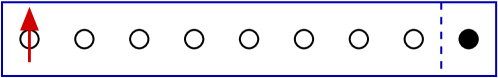
Figure 6: Schematic depiction of the NRG procedure.

3.2.3 Renormalization Group Flow and Fixed Points

In order to understand the behavior of a system within the renormalization group in general, one searches for fixed points of the renormalization group transformation Wilson (1975), defined by

$${\cal R}[H^{*}]=H^{*}\;.$$ (58)

In analytic variants of the renormalization group, the behavior of the Hamiltonian $H$ is generally parameterized by a small number of coupling constants. Finding fixed points then amounts to finding stationary points in the flow equations governing these coupling constants. In the NRG, identifying fixed points is little more subtle: in practice, when the first $p$ rescaled energy levels $E_{p}^{L}$ are independent of $L$ for a particular (appropriately chosen) range of $L$, one identifies a fixed point. Some insight into the physics of the problem is usually necessary to choose appropriate ranges of $p$ and $L$. Once fixed points are identified, the physicical behavior governed by the fixed point is determined by the structure of the low-lying eigenstates. Note that such behavior is not guaranteed for a more general tight-binding Hamiltonian.

For the Kondo problem (and the SIAM in appropriate parameter regimes), two fixed points can be clearly identified; one associated with the behavior of model (54) at $J=0$ and one with its behavior at $J=\infty$. In both cases, the behavior at the fixed point is easy to understand: for $J=0$, the impurity is uncoupled to the conduction band and the excitation energies are those of the non-interacting tight-binding band extending from 0 to $L$. For $J=\infty$, the impurity forms an infinitely tightly bound singlet with site 0 of the tight-binding chain, effectively removing it from the system. The excitation energies relative to the ground state are therefore those of a chain extending from 1 to $L$, i.e., the excitation spectrum for $H_{L}(J=\infty)$ is the same as that for $H_{L-1}(J=0)$. An additional complication is that the nature of the spectrum for $H_{L}(J=0)$ depends on whether $L$ is even or odd; the asymptotic values of the scaled excitation energies are different for even and odd $L$ are different, even in the limit of large $L$. This can be taken into account, however, by always applying a sequence of two renormalization group transformations, i.e., by replacing $\cal R$ with ${\cal R}^{2}$ in (58) to determine the fixed points and then considering the odd $L$ and even $L$ cases separately. In fact, the crossover from the $J=0$ fixed point to the $J=\infty$ fixed point amounts to a reversal of the behavior for odd and even $L$ because the zeroth lattice site is effectively removed from the chain at the strong coupling fixed point. For details on the structure of the excitation energies, see Refs. Wilson (1975); Hewson (1997); Krishna-murthy et al. (1980).

Numerically, one finds that for small $L$ and small but finite $J$, the structure of the excitations is that of the $J=0$ fixed point, whereas for large $L$ the structure is that of the $J=\infty$ fixed point. Stability analysis, which can be carried out analytically near the fixed points, shows that the effective Hamiltonian for the weak-coupling fixed point has a marginal operator, indicating that it is unstable, while the effective Hamiltonian for the strong-coupling fixed point has no relevant operators, indicating that it is stable Wilson (1975); Krishna-murthy et al. (1980); Hewson (1997), in agreement with the behavior observed in the NRG. The renormalization group flow from the unstable $J=0$ fixed point to the stable $J=\infty$ fixed point is depicted in Fig. 7.

Figure 7: Renormalization group flow diagram for the Kondo model.

3.2.4 Calculation of Thermodynamic Properties

Thermodynamic quantities such as the specific heat or the impurity susceptibility can be easily calculated within the NRG if the range of validity of the excitation spectrum is taken into account. Generally, one is interested in the impurity contribution to the thermodynamic quantities, derived from the impurity free energy $F_{\rm imp}(T)=-k_{B}T\ln Z/Z_{c}$, where $Z_{c}$ is the exactly calculable partition function for the noninteracting conduction band. If the entire eigenvalue spectrum were known, the partition function would be given by $Z(T)={\rm Tr}\exp(-\tilde{H}^{K}/k_{B}T)$. However, at a particular stage of the NRG, what one can calculate is the partition function for the truncated lattice

$$Z_{L}(T)\equiv{\rm Tr}e^{-\tilde{H}_{L}/k_{B}T}=\sum_{n}e^{-\tilde{E}^{L}_{n}/k_{B}T}=\sum_{n}e^{-D_{L}E^{L}_{n}/k_{B}T}\;.$$ (59)

Evidently, $Z_{L}(T)$ can only be a good approximation for $Z(T)$ when the temperature for a particular system size $T_{L}$ is chosen so that $k_{B}T_{L}\ll\alpha D_{L}$, the largest energy scale accurately described by $\tilde{H}_{L}$. We previously argued that the minimum energy is set by $D_{L}$; the error made in substituting $Z_{L}$ for $Z$ in calculating impurity properties has been more rigously estimated to be $D_{L}/\Lambda k_{B}T$ in Ref.  Krishna-murthy et al. (1980). Therefore, the valid temperature range for a given $L$ is set by

$$\Lambda^{-1}\ll\frac{k_{B}T_{L}}{D_{L}}\ll\alpha\;,$$ (60)

where $\alpha$ depends on $m$ and $\Lambda$. In practice, $k_{B}T_{L}\approx D_{L}$ is a reasonable choice.

Experimentally interesting quantities are the impurity specific heat

$$C_{\rm imp}=-T\frac{\partial^{2}}{\partial T^{2}}F_{\rm imp}(T)$$ (61)

and the magnetic susceptibility at zero field due to the impurity

$$\chi_{\rm imp}=\frac{(g\mu_{B})^{2}}{k_{B}T}\left[\frac{{\rm Tr}(S_{L}^{z})^{2}\,e^{-\tilde{H}/k_{B}T}}{Z}-\frac{{\rm Tr}(S_{L}^{z,c})^{2}\,e^{-\tilde{H}_{c}/k_{B}T}}{Z_{c}}\right]$$ (62)

where $S_{L}^{z}$ and $S_{L}^{z,c}$ are the $z$-components of the total spin on the $L$-site chain with and without the impurity spin, respectively. The Hamiltonian $H_{c}$ is that of the noninteracting conduction band. The high- and low-temperature limits, as well as the leading behavior around these limits have been calculated analytically. These limits can serve as a check of the accuracy of the NRG calculations. For a more complete depiction and discussion of results for thermodynamic properties, see Refs. Wilson (1975); Krishna-murthy et al. (1980); Hewson (1997).

3.2.5 Dynamical Observables and Transport Properties

Dynamical properties, both at zero and at finite temperature, can also be calculated within the NRG procedure. To be concrete, we will discuss perhaps the most experimentally interesting quantity, the impurity spectral function at zero temperature (for simplicity):

$$A(\omega)=-\frac{1}{\pi}\,{\rm Im}\,G(\omega+i\eta)\;,$$ (63)

where

$$G(t)=-i\langle\psi_{0}|\,T\,d(t)d^{\dagger}(0)\,|\psi_{0}\rangle$$ (64)

is the retarded impurity Green function [c.f. Eqs. (28)-(31)]. For finite $L$, it is convenient to calculate the spectral weight within the Lehmann representation

$$A_{L}(\omega)=\frac{1}{Z_{L}}\sum_{p}\left|\langle p|d^{\dagger}_{\sigma}|0\rangle\right|^{2}\delta(\omega-E_{p}+E_{0})\,+\,\left|\langle 0|d^{\dagger}_{\sigma}|p\rangle\right|^{2}\delta(\omega+E_{p}-E_{0})\;.$$ (65)

Since the excitations out of the ground state for $\tilde{H}_{L}$ are well-represented in the energy range $D_{L}\leq\omega\leq\alpha D_{L}$, as discussed previously, $A(\omega_{L})\approx A(\omega)$ when $\omega$ is chosen to be within this range. In practice, a typical choice is $\omega=2\omega_{L}$ where $\omega_{L}\equiv k_{B}T_{L}=D_{L}$. One usually uses Eq. (65) directly to calculate the spectrum, rather than the more sophisticated methods such as the Krylov method outlined in Sec. 2.4.1 or the correction vector method outlined in Sec. 2.4.2 because all eigenstates within the required range of excitation energy are available within the NRG procedure; it is then easy to calculate the poles and matrix elements within this range. Note that the result obtained is a set of positions and weights of $\delta$-functions; in order to compare with continuous experimental spectra, they must be broadened. Typical choices for a broadening function are Gaussian or Logarithmic Gaussian distributions of width $D_{L}$ Sakai and Hasegawa (1999); Costi (1999).

One interesting application of impurity problems comes about in the context of the Dynamical Mean Field Theory (DMFT), in which a quantum lattice model such as the Hubbard model is treated in the limit of infinite dimensions Metzner and Vollhardt (1989); Jarrell (1992); Georges et al. (1996). The problem can be reduced to that of a generalized SIAM interacting with a bath or host. The fully frequency-dependent impurity Green function of this generalized SIAM must then be calculated in order to iterate a set of self-consistent mean-field equations. Various methods can be used to solve the impurity problem including perturbation theory, exact diagonalization, quantum Monte Carlo, dynamical DMRG (DDMRG), and the NRG Georges et al. (1996); Bulla et al. (1998). Dynamical properties at finite temperature can be calculated using similar considerations, as long as the additional energy scale $k_{B}T$ is taken into account Costi and Hewson (1991, 1992, 1993); Costi (1999). In particular, the procedure outlined above can be used as long as frequencies $\omega>k_{B}T$ are considered. For $\omega<k_{B}T$, additional excitations at higher energies than $D_{L}<\omega<\alpha D_{L}$ become important. Frequencies in this range can then be handled using a smaller $L$ so that $\omega_{L}<K_{B}T$. Since transport properties such as the resistivity $\rho(T)$ can be formulated in terms of integrals over frequency of frequency-dependent dynamical correlation functions Costi and Hewson (1993), these methods can also be used to calculate them.

3.3 Numerical RG for Quantum Lattice Problems

There are a number of quantum lattice problems that have Hamiltonians whose structure is formally similar to the tight-binding Hamiltonian for the Kondo model (54) such as the Hubbard model (8) or the Heisenberg model (10) in one dimension. While one could consider carrying out a variation of the NRG procedure on these models in order to perform an approximate exact diagonalization on a finite lattice, the physically interesting case is the one in which the couplings between nearest-neighbor sites are all equal. This amounts to setting $\Lambda=1$ in the Kondo case, the point at which the convergence of the NRG method breaks down completely because the identification of the length $L$ with the energy scale is lost. Nevertheless, adaptations of the NRG procedure were applied to small Hubbard chains Bray and Chui (1979), obtaining an error in the ground-state energy of approximately 10% after 4 renormalization group steps. Later work on the spin-1 Heisenberg chain obtained an error of approximately 3% in the ground-state energy of the $L=18$ chain Xiang and Gehring (1993). It is important to note that such calculations are variational so that quantities which characterize the long distance behavior such as correlation functions which depend on the wave function can have much larger errors than the error in the energy. Finally, an adaptation of the NRG procedure to a two-dimensional noninteracting electron gas was used to study the Anderson localization problem in two dimensions Lee (1979). The result obtained was that the system undergoes a localization-delocalization transition as a function of disorder strength, a result later discovered to be incorrect: there is no transition because two is the lower critical dimension Lee and Fisher (1981); Abrahams et al. (1979).

3.4 Numerical RG for a Noninteracting Particle

More insight into the breakdown of the NRG procedure for one-dimensional lattice problems with non-decaying couplings can be gained by applying a variant of the procedure to the problem of a single particle on a tight-binding chain, Eq. (6). We consider the Hamiltonian in the formulation

$$H=-\sum_{\ell=1}^{L-1}\left(~{}|\ell\rangle\langle\ell+1|+|\ell+1\rangle\langle\ell|~{}\right)+2\sum_{\ell=1}^{L}|\ell\rangle\langle\ell|\;,$$ (66)

where that state $|i\rangle$ represents an orbital localized on site $\ell$. In a matrix representation, this Hamiltonian is tridiagonal and is equivalent to a discretized second derivative operator, $-\partial^{2}/\partial x^{2}$. Note that Hamiltonian (66) does not include a nonzero matrix element between sites 1 and $L$, so that fixed boundary conditions have been applied to the chain, i.e., the wave function is required to vanish at the ends. We modify the Wilson NRG procedure slightly to take into account that we are treating a simpler, noninteracting system. There are two significant changes: first, we put together two equal-sized systems (called “blocks”) rather than just adding a site because the dimension of the Hilbert space grows more slowly than in an interacting system: linearly rather than exponentially with the length. Second, the mechanics of putting two blocks together is simpler in the interacting system.

In terms of the procedure outlined in Sec. 3.2.2, the diagonalization of the Hamiltonian, step 1), and the transformation of the relevant operators using $\mathbf{O}_{L}$, a matrix whose columns are the $m$ eigenvectors of $\mathbf{H}_{L}$ with the lowest eigenvalues, [step 2)] are carried out as before. The procedure is somewhat simplified because of the less complicated structure of Hamiltonian (66); for example, there are no $S^{z}$ and $N$ quantum numbers which decouple sectors of $\mathbf{H}$. The operators to be transformed are the Hamiltonian for a block $\bar{\mathbf{H}}_{L}=\mathbf{O}^{\dagger}_{L}\mathbf{H}_{L}\mathbf{O}_{L}$ which is diagonal and $\bar{\mathbf{T}}_{L}=\mathbf{O}^{\dagger}_{L}\mathbf{H}_{L}\mathbf{O}_{L}$, where $\mathbf{T}_{L}$ represents the connection between the blocks. The procedure is conveniently started at $L=1$ for which $\mathbf{H}_{1}=2$ and $\mathbf{T}_{L}=-1$ can be represented as $1\times 1$ matrices. Matrix representations of a system of size $2L$ are then formed [step 3)] as

$$\mathbf{H}_{2L}=\left(\begin{array}[]{cc}\bar{\mathbf{H}}_{L}&\bar{\mathbf{T}}_{L}\\ \bar{\mathbf{T}}^{\dagger}_{L}&\bar{\mathbf{H}}_{L}\\ \end{array}\right)$$ (69)

and

$$\mathbf{T}_{2L}=\left(\begin{array}[]{cc}0&0\\ \bar{\mathbf{T}}_{L}&0\\ \end{array}\right)\;.$$ (72)

The procedure is then iterated [step 4)], doubling the size of the system at each step. The matrix to be diagonalized, $\mathbf{H}_{2L}$, is of size $2m\times 2m$ at a general step, and the truncation is to an $m\times m$ matrix, i.e., one half of the Hilbert space is discarded. Note that the procedure is exact for the first few steps, as long as $m\leq L$.

Table 3: Lowest energies after 10 blocking transformations for the noninteracting single particle on a 1-D chain with fixed boundary conditions, keeping up to $m=8$ states.

	Exact	Wilson	Fixed-Free
$\ E_{0}\$	$\;2.3508\times 10^{-6}\;$	$\;1.9207\times 10^{-2}\;$	$\;2.3508\times 10^{-6}\;$
$\ E_{1}\$	9.4032$\;\times 10^{-6}\;$	1.9209$\;\times 10^{-2}\;$	$9.4032\times 10^{-6}$
$\ E_{2}\$	$2.1157\times 10^{-5}$	$1.9214\times 10^{-2}$	$2.1157\times 10^{-5}$
$\ E_{3}\$	$3.7613\times 10^{-5}$	$1.9217\times 10^{-2}$	$3.7613\times 10^{-5}$

As shown in the first two columns of Table 3, the accuracy of the eigenvalues obtained breaks completely after a moderate number of steps. The failure of the NRG for this simple problem as well as the reason for the failure was pointed out by Wilson in 1986 wil (1986). For a particular $L$, the eigenfunctions have the form

$$\psi^{L}_{n}(\ell)\propto\sin\left(\frac{n\pi\ell}{L+1}\right)\;,\hskip 56.9055ptn=1,\ldots,L$$ (73)

because fixed boundary conditions have been applied to the system. In one iteration of the NRG procedure, a linear combination of the $\psi^{L}_{n}(\ell)$ for $n\leq m$ are used to form an approximation to $\psi^{2L}_{n}(\ell)$. As depicted in Fig. 8, the boundary conditions that are applied to $\mathbf{H}_{L}$ lead to a non-smooth “dip” in the wave function in the middle of the block of size $2L$ when the NRG transformation is carried out. Clearly, this dip can only be removed by forming a linear combination of almost all of the $\psi^{L}_{n}(\ell)$. The lesson that is learned, then, is that how the boundaries of the blocks are treated in the NRG procedure is crucial: a more general treatment is necessary to formulate a numerically accurate real-space NRG procedure for short-ranged quantum lattice models.

Figure 8: The lowest eigenstates of two 8-site blocks (solid circles) and a 16-site block (open squares) for the one-dimensional tight–binding model with fixed boundary conditions.

4 From the NRG to the Density Matrix Renormalization Group

4.1 Better Methods for the Noninteracting Particle

Perhaps the most obvious way of improving the NRG, at least for the single tight-binding particle, is to apply a more general set of boundary conditions to the system to be diagonalized. For example, one can apply fixed (vanishing wave function in the continuum limit) or free boundary conditions (vanishing first derivative) by forming the matrix

$$\mathbf{H}^{bb^{\prime}}_{2L}=\left(\begin{array}[]{ccc}\bar{\mathbf{H}}^{b,\rm fixed}_{L}&&\bar{\mathbf{T}}_{L}\\ \bar{\mathbf{T}}_{L}^{\dagger}&&\bar{\mathbf{H}}^{\rm fixed,b^{\prime}}_{L}\\ \end{array}\right)$$ (76)

when putting two blocks together, where the boundary condition $b$ can be fixed or free White and Noack (1992). For example,

$$\mathbf{H}^{\rm free,fixed}_{L=2}=\left(\begin{array}[]{ccc}1&&-1\\ -1&&2\\ \end{array}\right)\;.$$ (79)

The Hamiltonian $\mathbf{H}^{bb^{\prime}}_{2L}$ can then be diagonalized for all 4 combinations of boundary conditions to obtain a more general set of basis functions, albeit an overcomplete set which is not orthogonalized. However, if only a small number (e.g., $m/4$) of eigenstates from each set $\{b,b^{\prime}\}$ are kept in the transformation matrix $\mathbf{O}_{L}$, the columns of $\mathbf{O}_{L}$ can then be orthogonalized numerically using the Gram–Schmidt procedure, resulting in an undercomplete orthogonal transformation, as before. The matrices $\bar{\mathbf{H}}^{bb^{\prime}}_{L}=\mathbf{O}_{L}^{\dagger}\mathbf{H}^{bb^{\prime}}_{L}\mathbf{O}_{L}$ and $\bar{\mathbf{T}}_{L}=\mathbf{O}_{L}^{\dagger}\mathbf{H}^{bb^{\prime}}_{L}\mathbf{O}_{L}$ must then be transformed to prepare for the next step. Note that $\bar{\mathbf{H}}^{bb^{\prime}}_{L}$ is not diagonal.

As can be seen in Table 3, this “combination of boundary conditions” method works astoundingly well, producing the first few eigenvalues to almost machine accuracy for a 2048-site lattice, keeping only $m=8$ states White and Noack (1992). However, the crucial question is whether the technique can be generalized to interacting many-particle systems. Unfortunately, no good method has been found to extend these “combination of boundary conditions” methods. The reason is that it is not clear that an appropriately general set of boundary conditions can be found for a many-particle wave function, which is a complicated function of the coordinates of all the particles.

However, another method developed in Ref. White and Noack (1992), called the superblock method, can be generalized to interacting systems. Rather than applying a general set of boundary conditions to a block of size $L$, this method forms a new basis for $\bar{\mathbf{H}}_{2L}$ and $\bar{\mathbf{T}}_{2L}$ based on the idea that these blocks will eventually make up part of a larger system. In order to do this, a “superblock” (with periodic boundary conditions) made up of $p>2$ blocks is formed and diagonalized. For example,

$$\mathbf{H}^{p=4}_{2L}=\left(\begin{array}[]{cccc}\bar{\mathbf{H}}_{L}&\bar{\mathbf{T}}_{L}&0&\bar{\mathbf{T}}^{\dagger}_{L}\\ \bar{\mathbf{T}}^{\dagger}_{L}&\bar{\mathbf{H}}_{L}&\bar{\mathbf{T}}_{L}&0\\ 0&\bar{\mathbf{T}}^{\dagger}_{L}&\bar{\mathbf{H}}_{L}&\bar{\mathbf{T}}_{L}\\ \bar{\mathbf{T}}_{L}&0&\bar{\mathbf{T}}^{\dagger}_{L}&\bar{\mathbf{H}}_{L}\\ \end{array}\right)\;.$$ (84)

The transformation $\mathbf{O}_{2L}$ is then made up by projecting the $m$ lowest–lying eigenstates of $\mathbf{H}^{p}_{2L}$ onto the coordinates of the first two blocks, and then orthonormalizing its columns. In other words, if $u^{\alpha}_{j}$ (with $j=1,\ldots,4m$) is an eigenvector of $\mathbf{H}^{4}_{2L}$, then a nonorthonormalized column vector of $\mathbf{O}_{2L}$ is composed of the first $2m$ elements, $j=1,\ldots,2m$, of $u^{\alpha}_{j}$, assuming $\bar{\mathbf{H}}_{L}$ is an $m\times m$ matrix. This new basis is used to transform $\bar{\mathbf{H}}_{2L}=\mathbf{O}^{\dagger}_{2L}\mathbf{H}_{2L}\mathbf{O}_{2L}$ and $\bar{\mathbf{T}}_{2L}=\mathbf{O}^{\dagger}_{2L}\mathbf{T}_{2L}\mathbf{O}_{2L}$, as defined in (69) and (72).

The superblock method yields good results for the single-particle tight-binding chain, albeit not as accurate as the fixed-free variant of the combination of boundary conditions method White and Noack (1992). As one might expect, the method also becomes more accurate as the number of blocks making up the superblock, $p$, is increased. If $p$ can be made arbitrarily large, it can be adjusted so that one is simply carrying out an exact diagonalization of a system of the desired size. Since the additional blocks in the superblock allow fluctuations at the boundaries of the blocks whose wave functions are used in the renormalization group blocking step, this method is more promising to apply to interacting systems: such fluctuations should also treat the boundaries of blocks of a many-body system in a more general way. For a single-particle system, the projection of the wave function of the superblock onto the subsystem of interest is trivial: it is a one-to-one projection because the Hilbert space of the superblock is a direct sum of that of its subsystems. This projection is more complicated for a many-body system: one state of the superblock can project onto many states of a subsystem because the Hilbert space grows exponentially, as a direct product of that of the subsystems.

It is also possible to treat the single particle on a tight-binding chain, Hamiltonian (66), using an algorithm that is a direct adaptation of the DMRG for interacting systems Noack and White (1999). This algorithm is linear in the system size $L$ and involves diagonalizing only a $4\times 4$ matrix at each DMRG step Martín-Delgado et al. (1999). Since the single-particle algorithm contains the essential ingredients of the DMRG algorithm for interacting systems, we believe that understanding the single-particle algorithm is useful in gaining insight into the algorithm for interacting systems. We therefore encourage the reader to work through the example implementation of this algorithm Noack and White (1999) and to examine a similar program which is part of the ALPS application library alp (ALPS, see cond-mat/0410407).

4.2 Density Matrix Projection for Interacting Systems

In the following sections, we will discuss how to generalize the superblock method to interacting systems. This will lead to the density matrix renormalization group method (DMRG), one of the most efficient numerically exact methods for one-dimensional strongly correlated quantum systems. The reader is encouraged to supplement the discussion given here with White’s original papers White (1992, 1993a) and other introductory and review articles on the method Peschel et al. (1999a); Hallberg (2004); Schollwöck (2005). In addition, a collection of papers using the DMRG or treating subjects connected to the DMRG can be found in Ref. nis (maintained by T. Nishino, updated daily), a survey is presented in Ref. eri (maintained by E. Jeckelmann).

As we have seen in Sec. 4.1, the crucial step of the superblock method is a projection of the wave function of the superblock onto a subsystem, consisting of two identical blocks for the algorithm for the noninteracting particle. Here we consider how to carry out such a projection for a many-body wave function in an optimal way. In order to do this, we briefly review the general quantum mechanical description of a system divided into two parts.

The density matrix is the most general description of a quantum mechanical system because, in contrast to a description in terms of the wave function, it can be used to describe a system in a mixed state as well as in a pure state Laundau and Lifshitz (1965); Feynman (1972). For a general, mixed state, the density matrix of a system is given by

$$\rho=\sum\limits_{\alpha}\,C_{\alpha}\,|\Psi_{\alpha}\rangle\langle\Psi_{\alpha}|,$$ (85)

where the coefficients $C_{\alpha}$ are the weights of the states in the mixed ensemble and are normalized so that $\mbox{Tr}\;\rho=1$. The density matrix for a system in a pure state would have just one term in the sum. Given $\rho$, a subsystem $A$ can be described by tracing out the degrees of freedom $|j\rangle$ of the rest of the system, yielding the reduced density matrix

$$\rho_{A}=\mbox{Tr}_{|j\rangle}\rho\;.$$ (86)

The eigenstates of $\rho_{A}$ form a complete basis for the subsystem $A$; its eigenvalues $w_{\alpha}$ give the weight of state $\alpha$ in the ensemble and carry the information about the entanglement of the subsystem with the rest of the system. The amount of entanglement can be quantified by the mutual quantum information entropy

$$S(\rho) = -\mbox{Tr}_{|j\rangle}\left(\rho\log\rho\right)$$ (87)

$$= -\sum_{\alpha}w_{\alpha}\log w_{\alpha}\;.$$

This feature gives an interrelation between the DMRG and quantum information theory as discussed in more detail in Sec. 6.7. If a system in a pure state $|\psi\rangle$ is divided into two parts (A and B), $|\psi\rangle$ can be expressed in terms of the eigenstates of the reduced density matrices of part A, $|\phi_{\alpha}\rangle$, and part B, $|\chi_{\alpha}\rangle$ using the Schmidt decomposition Schmidt (1907); pre (”Quantum Computation”, lecture notes by J. Preskill)

$$|\psi\rangle=\sum_{\alpha}\sqrt{w_{\alpha}}\;|\phi_{\alpha}\rangle\;|\chi_{\alpha}\rangle\;.$$ (88)

Here the sum is over the nonzero eigenvalues $w_{\alpha}$ of the density matrices of either part, which can be shown to be the same. The behavior of the eigenvalues $w_{\alpha}$ with $\alpha$ depends on the wave function considered and on how the two subsystems are chosen. If only a small number (i.e., substantially less than the dimension of the smallest of the two density matrices) of the $w_{\alpha}$ are nonzero, $|\psi\rangle$ can be represented exactly by the sum over the corresponding states. If the $w_{\alpha}$ fall off sufficiently rapidly with $\alpha$, $|\psi\rangle$ can be well approximated by truncating the sum in Eq. (88) to the $m$ eigenstates of the density matrix with the largest eigenvalues. This is the case for, e.g., one-dimensional quantum many-body systems with a gapped spectrum, i.e., away from a quantum critical point, for which $w_{\alpha}$ falls off exponentially (see the discussion of this topic in Ref. Schollwöck (2005)). A useful approximation can be achieved if $m$ can be taken to be much smaller than the dimension of the eigenbasis of the density matrix. This approximation can be shown to be optimal in the sense of a least-squares minimization of the differences between the exact $|\psi\rangle$ and the approximate one White (1993a) and is equivalent to the singular value decomposition Press et al. (1993). Finally, if the $w_{\alpha}$ fall off too slowly or not at all, a truncation of the Schmidt decomposition becomes a bad approximation for $|\psi\rangle$. The worst case is when all the $w_{\alpha}$ are equal, which occurs for a maximally entangled state. A representation optimized for multiple states rather than just $|\psi\rangle$ can be constructed by including additional states in the density matrix, Eq. (85) with appropriate weights $C_{\alpha}$. The Schmidt decomposition, Eq. (88) is then no longer applicable and the approximation to a particular state for a given $m$ will become less accurate.

A measure for the error of this approximation is the sum over the weights of the discarded density-matrix eigenstates,

$$\varepsilon_{\rm discard}=\sum_{m}^{N}w_{\alpha},$$ (89)

with $N$ the dimension of the system’s Hilbert space. This is called the discarded weight. Thus, using the basis of density matrix eigenstates, an “optimal” description for a quantum many-body system can be found (for details, see Ref. Noack and White (1999)). In the usual case, the calculation is performed in order to obtain the ground state of the system in a particular symmetry sector of the Hilbert space, thus only one target state is kept and the density matrix, Eq. (85), has just one term in the sum. Here and in the following, we will therefore discuss the procedure for a calculation with a single target state; the generalization to multiple target states is straightforward.

The basic procedure to carry out the truncation is then:

1. Obtain the ground state $|\psi\rangle$ of a finite lattice system using an iterative diagonalization procedure (e.g., the Lanczos or Davidson algorithms).

2. Divide the system in two and obtain the $m$ most important eigenstates of the reduced density matrix of one of the subsystems.

3. Transform the system block into the new (approximate) basis with only $m$ states.

The DMRG is a numerically implemented variational method based on this truncation. In the following, the implementation of this method is discussed. For pedagogical example implementations for the noninteracting case, we refer the reader to Refs. alp (ALPS, see cond-mat/0410407); Noack and White (1999).

4.3 DMRG Algorithms

The goal in formulating DMRG algorithms is to embed an NRG-like iterative buildup and truncation of a system, termed “system block”, in a larger system, the superblock. As described in the previous section, an iterative diagonalization is carried out on the superblock to obtain the ground state and possibly some other states, and the eigenstates of the corresponding reduced density matrix with the largest weights are used to form a new truncated basis for the system block. In order to construct DMRG algorithms, two elements of the procedure must still be formulated: how the system block is built up, i.e., how degrees of freedom are added, and how the remainder of the superblock, termed “environment” or “environment block”, is chosen. In the NRG a single site at a time is added to the system, allowing a substantial fraction of the energy eigenstates ($1/N_{\ell}$, where $N_{\ell}$ is the number of states on site $\ell$) to be kept at each step. In the DMRG, it is also important to minimize the number of degrees of freedom, especially since the system to be diagonalized, the superblock, contains many additional degrees of freedom in the environment block. Therefore, a single site is added to the system block at each step in almost all variants of the DMRG algorithm. There is more freedom to choose how the environment block is constructed: the algorithms generally fall into two classes, depending on how the superblock evolves with iteration. In the infinite system procedure, the size of the superblock increases at each step in a fashion reminiscent of the NRG, and in the finite system procedure, the environment block is chosen so that the size of the superblock remains constant, allowing an iterative improvement of the wave function or wave functions for one particular finite system.

4.3.1 Infinite System Algorithm

In the infinite system algorithm, the environment block is chosen to be a reflection of the system block, (usually) including the added site. Therefore, the superblock grows by two sites at each iteration (as opposed to one site in the NRG) and the algorithm can be used to scale towards the infinite-system fixed point, or, as we will see, can be used to build up an initial approximation to a system of a particular size, which can then be further improved with the finite system procedure. Such additional finite-system iteration is necessary for most systems because the infinite-system algorithm is not guaranteed to achieve variational convergence with the number of states kept Noack and White (1999); Boschi and Ortolani (2004).

Figure 9: Superblock configuration for the infinite system algorithm.

The infinite system algorithm for the calculation of the ground state of a one-dimensional reflection symmetric lattice proceeds as follows.

1. Form a superblock containing $L$ sites which is small enough to be exactly diagonalized.

2. Diagonalize the superblock Hamiltonian $H^{\rm super}_{L}$ numerically, obtaining only the ground state eigenvalue and eigenvector $\psi$ using the Lanczos or Davidson algorithm.

3. Form the reduced density matrix $\rho_{ii^{\prime}}$ for the current system block from $\psi$ using $\rho_{ii^{\prime}}=\sum_{j}\psi^{*}_{ij}\psi_{i^{\prime}j}$, where $|i\rangle$ is the basis of the system block of size $\ell+1$, $|j\rangle$ the basis of the corresponding environment block, and $\psi_{ij}=\langle i|\,\langle j|\psi\rangle$. Note that $\ell^{\prime}=\ell=L/2-1$.

4. Diagonalize $\rho_{ii^{\prime}}$ with a dense matrix diagonalization routine to obtain the $m$ eigenvectors with the largest eigenvalues.

5. Construct the Hamiltonian matrix $\mathbf{H}_{\ell+1}$ of the new system block (i.e. the left block $A+s$) and other operators needed in the course of the iteration (e.g. observables). Transform them to the reduced density matrix eigenbasis using $\bar{\mathbf{H}}_{\ell+1}^{\alpha}=\mathbf{O}^{\dagger}_{L}\mathbf{H}_{\ell+1}^{\alpha}\mathbf{O}_{L}$, $\bar{\mathbf{A}}_{\ell+1}=\mathbf{O}^{\dagger}_{L}\mathbf{A}_{\ell+1}\mathbf{O}_{L}$, etc., where the columns of $\mathbf{O}_{L}$ contain the $m$ eigenvectors of $\rho_{ii^{\prime}}$ with the highest eigenvalues, and $\mathbf{A}_{\ell+1}$ is an operator in the system block.

6. Form a superblock of size $L+2$ using $\bar{H}_{\ell+1}$, two single sites and $\bar{H}^{R}_{\ell+1}$.

7. Repeat starting with step 2, substituting $H^{\rm super}_{L+2}$ for $H^{\rm super}_{L}$.

The implementation details for the individual steps will be described in Sec. 5.1. In order to obtain an efficient program, bases and operators should be decomposed according to the symmetries of the Hamiltonian whenever possible. For an introduction to the use of symmetries within the DMRG framework, see Ref. Malvezzi (March 2003).

This procedure has been formulated to obtain only the ground state, but it is easy to extent it to multiple target states by constructing additional states during step 2, either by continuing the diagonalization to obtain excited states or by applying operators to $|\psi\rangle$. These additional states are then mixed into the reduced density matrix in step 3 with appropriate weights, as discussed in Sec. 4.2.

Here a reflection-symmetric one dimensional system has been assumed. It is possible to generalize the infinite system algorithm to non-reflection-symmetric lattices by building up the left half and the right half of the system alternately. However, such algorithms have not been particularly important because the finite system algorithm, discussed below, can treat such cases and can be generalized to systems that are not one-dimensional chains.

The results of the procedure are the energies and wave functions obtained in step 2. At this point, matrix elements of operators within a state and between states can be calculated, provided that the operators have been formed in the appropriate basis, i.e., the same basis in which $|\psi\rangle$ is represented in step 2.

4.3.2 Finite System Algorithm

The infinite system method has the weakness that the wave function targeted at each step is different because the lattice size is different. This can lead to poor convergence or complete lack of convergence with $m$ if the wave function changes qualitatively between steps. This can occur for states with some incommensuration with the lattice such as, for example, fermions with a nonintegral filling or excited states characterized by a particular wavevector.

Therefore, an algorithm in which the same finite system is treated at each step is very useful. Instead of convergence to an infinite-system fixed point with iteration, there is variational convergence to the wave function or set of wave functions for a particular finite system. Such an algorithm can be formulated by choosing a block of appropriate size from a previous step as the environment block.

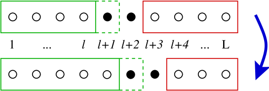
Figure 10: A schematic depiction of a step in the finite-system algorithm.

The finite system algorithm for finding the ground state on a one-dimensional lattice proceeds as follows:

1. Carry out the infinite system algorithm until the superblock reaches size $L$, storing $\bar{H}_{\ell}$ and the operators needed to connect the blocks at each step.

2. Carry out steps 3-5 of the infinite system algorithm to obtain $\bar{H}_{\ell+1}$. Store it. (Now $\ell\neq\ell^{\prime}$.)

3. Form a superblock of size $L$ using $\bar{H}_{\ell+1}$, two single sites and $\bar{H}^{R}_{\ell^{\prime}-1}$. The superblock configuration is shown in Fig. 10 where $\ell^{\prime}=L-\ell-2$.

4. Repeat steps 1-2 until $\ell=L-3$ (i.e. $\ell^{\prime}=1$). This is the left to right phase of the algorithm.

5. Carry out steps 3-5 of the infinite system algorithm, reversing the roles of $\bar{H}_{\ell}$ and $\bar{H}^{R}_{\ell^{\prime}}$, i.e. switch directions to build up the right block and obtain $\bar{H}^{R}_{\ell^{\prime}+1}$ using the stored $\bar{H}_{\ell}$ as the environment. Store $\bar{H}^{R}_{\ell^{\prime}+1}$.

6. Form a superblock of size $L$ using $\bar{H}_{\ell-1}$, two single sites and $\bar{H}^{R}_{\ell^{\prime}+1}$.

7. Repeat steps 4-5 until $\ell=1$. This is the right to left phase of the algorithm.

8. Repeat starting with step 1.

This procedure is illustrated schematically in Fig. 10.

One iteration of the outermost loop is usually called a finite-system iteration or finite-system sweep. If the lattice is reflection symmetric, the procedure can be shortened by reversing direction at the reflection symmetric point, $\ell=L/2-1$, i.e., by using the reflection symmetry to interchange the role of the left and right blocks at this point. In this formulation, we have assumed that the infinite system algorithm can be carried out to build up the lattice to the desired size and to generate an initial set of environment blocks. If this is not the case, the finite system method can still be applied if a reasonable approximation is used for the environment block in the first finite-system sweep. The simplest such approximation is to use a null environment block, which is equivalent to the Wilson NRG procedure; a better one is to use a few exactly treated sites as the environment. As long as this initial procedure does not lead to a system block basis that is too bad, convergence is reached after a relatively small number of finite system iterations for most systems, typically between 2 and 10 for one-dimensional systems.

Note that, as in the infinite system algorithm, it is also possible to obtain results for several target states by mixing additional states into the density matrix in step 3.

We show an example of the behavior of the ground-state energy in the course of a DMRG run for the half-filled one-dimensional Hubbard model in Fig. 11. Note the convergence is clearly variational and that there is a significant downwards jump in the energy when the direction is changed at the middle of the chain in the finite system algorithm. This is due to a qualitative improvement in the representation of the system as the reflected system block can also be used as the environment block.

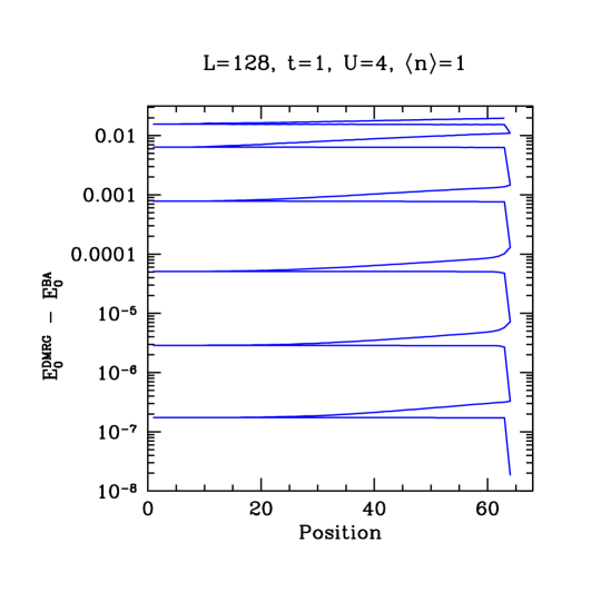
Figure 11: Ground-state energy $E_{0}^{\rm DMRG}$ obtained by the DMRG algorithm compared with the exact ground state energy from the Bethe Ansatz $E_{0}^{\rm BA}$ for the one-dimensional Hubbard model of length $L=128$ with $U/t=4$ at half-filling. “Position” refers to the position at which a site is added. The infinite system algorithm (not shown) followed by six sweeps of the reflection-symmetric version of the finite system algorithm are carried out.

Since its introduction thirteen years ago, the DMRG has become a standard method for obtaining the ground-state properties of one-dimensional short-range quantum lattice models. Among the first and most extensive areas of application have been spin chains with half-integral and integral spin White (1992, 1993a); White and Huse (1993), as well as frustrated spin chains White and Affleck (1996). One-dimensional fermionic systems Noack et al. (1994a, 1999); Manmana et al. (2004) have been treated in many variations. Since the amount of work done on such models is quite large, a comprehensive survey is beyond the scope of this pedagogical introduction; we refer the reader to Refs. Peschel et al. (1999a); Hallberg (2004); Schollwöck (2005) for further references.

5 The DMRG in Detail

5.1 Programming Details

In this section, we discuss the details of implementing the DMRG algorithm, paying particular regard to efficiency. We follow Ref. Peschel et al. (1999a) in that we take the one-dimensional Heisenberg model with nearest-neighbor exchange term

$${\bf S_{\ell}}\cdot{\bf S_{\ell+1}}=S^{z}_{\ell}S^{z}_{\ell+1}+\frac{1}{2}\left(S^{+}_{\ell}S^{-}_{\ell+1}+S^{-}_{\ell}S^{+}_{\ell+1}\right)$$ (90)

as an example. Any DMRG program will contain the following three crucial elements:

1. The addition of two blocks (usually the system block and a site).

2. The multiplication $H^{\rm super}|\psi\rangle$.

3. The basis transformation of relevant operators on a block to the truncated basis of density matrix eigenstates.

When two blocks are added, the part of the Hamiltonian internal to each block as well as all terms connecting the two blocks must be constructed. For the example, the terms that must be constructed are

$$\left[H_{12}\right]_{ii^{\prime};jj^{\prime}}= \left[H_{1}\right]_{ii^{\prime}}\delta_{jj^{\prime}}\;+\;\delta_{ii^{\prime}}\left[H_{2}\right]_{jj^{\prime}}\;+\;\left[S^{z}_{\ell}\right]_{ii^{\prime}}\left[S^{z}_{\ell+1}\right]_{jj^{\prime}}$$ (91)

$$\;+\;\frac{1}{2}\left(\left[S^{+}_{\ell}\right]_{ii^{\prime}}\left[S^{-}_{\ell+1}\right]_{jj^{\prime}}+\left[S^{-}_{\ell}\right]_{ii^{\prime}}\left[S^{+}_{\ell+1}\right]_{jj^{\prime}}\right)\;.$$

Note that the matrix representation of each operator appearing in Eq. (91) must be available in the current basis; such operators must be constructed and transformed in previous steps.

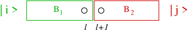
Figure 12: A schematic depiction of the addition of two blocks.

The multiplication $H^{\rm super}|\psi\rangle$ is the most time-consuming operation in the DMRG algorithm. The following is an efficient procedure to perform this operation within the framework of the DMRG; it should be considered to be the standard method. Assuming that the system is composed of two parts, the superblock Hamiltonian can be constructed using

$$\left[H^{\rm super}\right]_{ij;i^{\prime}j^{\prime}}=\sum\limits_{\alpha}A_{ii^{\prime}}^{\alpha}B_{jj^{\prime}}^{\alpha}\;,$$ (92)

where $\mathbf{A}^{\alpha}$ are the matrix representations of the appropriate operators on the left block, while the matrices $\mathbf{B}^{\alpha}$ are those on the right block. The index $\alpha$ iterates over all pairs of operators that are needed to construct the superblock Hamiltonian, as given in Eq. (91) for the example system. The product with the wave function in the appropriate superblock configuration then is

$$\sum\limits_{i^{\prime}j^{\prime}}\left[H^{\rm super}\right]_{ij;i^{\prime}j^{\prime}}\psi_{i^{\prime}j^{\prime}}=\sum\limits_{\alpha}\sum\limits_{i^{\prime}}A_{ii^{\prime}}^{\alpha}\sum\limits_{j^{\prime}}B_{jj^{\prime}}^{\alpha}\psi_{i^{\prime}j^{\prime}}\;.$$ (93)

For each $\alpha$, this expression is equivalent to the multiplication of three matrices

$$H^{\rm super}\psi=\sum\limits_{\alpha}\mathbf{A}^{\alpha}\left(\mathbf{B}^{\alpha}\psi^{T}\right)^{T}\;,$$ (94)

which can be carried out in order $m^{3}$ operations.

In the course of the DMRG procedure, all of the above matrices as well as the operators required to calculate desired observables must be transformed into the new truncated basis given by the $m$ density-matrix eigenvectors with largest weight. If the transformation matrix $O_{ij;\alpha}$ is composed of $m$ basis vectors $u^{\alpha}_{ij}$, the operator $A_{ij;i^{\prime}j^{\prime}}$ is transformed as

$$A_{\alpha\alpha^{\prime}}=\sum_{i,j,i^{\prime},j^{\prime}}O_{ij;\alpha}A_{ij;i^{\prime}j^{\prime}}O_{i^{\prime}j^{\prime};\alpha^{\prime}}\;,$$ (95)

leading to a reduction of the dimension of the matrix representing $A$ from $(m_{1}m_{2})\times(m_{1}m_{2})$ to $m\times m$.

In order to make the above procedures as efficient as possible, it is necessary to exploit the system’s Abelian symmetries. The sums over sets of states can be divided up into sectors corresponding to different quantum numbers. Once this is done, only the nonzero parts of the matrix representations of the operators which connect particular quantum numbers must be stored and the multiplications can be decomposed into sums over multiplications of these non-vanishing pieces. Use of non-Abelian symmetries is also possible, but is substantially more difficult McCulloch and Gulacsi (2000, 2001); McCulloch et al. (2001). In order to treat large systems and make $m$ as large as possible, it is also important to minimize the use of main memory. This can be done by storing the matrix representations of operators not currently needed on secondary storage. In particular, relevant operators for blocks that are not needed in the superblock configuration at a given step of the finite system procedure, but which will be needed in a subsequent step, need not be retained in primary storage.

5.2 Measurements

What are termed “measurements” in the DMRG framework are expectation values of operators calculated within a state or between states of the superblock, which are obtained in the iterative diagonalization step. The procedure is straightforward provided that the necessary operators are available in the appropriate basis. Given a state $\psi_{ij}$ of the two-block system, the single-site expectation value $\langle\psi|S^{z}_{\ell}|\psi\rangle$ is given by

$$\langle\psi|S^{z}_{\ell}|\psi\rangle=\sum_{i,i^{\prime},j}\psi^{*}_{ij}\,[S^{z}_{\ell}]_{ii^{\prime}}\,\psi_{i^{\prime}j}\;.$$ (96)

The matrix representation $[S^{z}_{\ell}]_{ii^{\prime}}$ is constructed when the site $\ell$ is added to the system block, and must be transformed at each subsequent step so that it is available in the basis $|i\rangle$.

For expectation values of operators on two different sites such as the correlation function $\langle\psi|S_{\ell}^{z}S_{m}^{z}|\psi\rangle$, how the operators are constructed depends on whether the two sites $\ell$ and $m$ are on the same or on different blocks. If they are located on different blocks, then the expectation value can be formed using

$$\langle\psi|S^{z}_{\ell}S^{z}_{m}|\psi\rangle=\sum_{i,i^{\prime},j,j^{\prime}}\psi^{*}_{ij}\,[S^{z}_{\ell}]_{ii^{\prime}}[S^{z}_{m}]_{jj^{\prime}}\,\psi_{i^{\prime}j^{\prime}}\;,$$ (97)

where $[S^{z}_{\ell}]_{ii^{\prime}}$ and $[S^{z}_{m}]_{jj^{\prime}}$ are the individual single-site operators. However, if $\ell$ and $m$ are on the same block, the expression

$$\langle\psi|S^{z}_{\ell}S^{z}_{m}|\psi\rangle\approx\sum_{i,i^{\prime},i^{\prime\prime},j}\psi^{*}_{ij}\,[S^{z}_{\ell}]_{ii^{\prime}}[S^{z}_{m}]_{i^{\prime}i^{\prime\prime}}\,\psi_{i^{\prime\prime}j}$$ (98)

is incorrect within the approximatation for $\psi_{ij}$ because the sum over $i^{\prime}$ extends over the current truncated basis rather than a complete set of states. The correct way to calculate the two-site expectation value is to use the relation

$$\langle\psi|S^{z}_{\ell}S^{z}_{m}|\psi\rangle=\sum_{i,i^{\prime},j}\psi^{*}_{ij}\,[S^{z}_{\ell}S^{z}_{m}]_{ii^{\prime}}\,\psi_{i^{\prime}j},$$ (99)

where the operator $[S^{z}_{\ell}S^{z}_{m}]_{ii^{\prime}}$ has been calculated at the appropriate step; this is correct within the variational approximation for $\psi_{ij}$. The general rule is, that compound operators internal to a block must be accumulated as the calculation proceeds. In this way, almost all correlation functions as well as more complicated equal-time expectation values can be calculated. The calculation of dynamical correlation functions and time-dependent quantities have been made possible by recent developments and will be discussed in Sec. 6.3 and Sec. 6.5, respectively.

5.3 Wave Function Transformations

The most time-consuming part of the DMRG algorithm is the iterative diagonalization of the superblock Hamiltonian. Here we discuss how to optimize this procedure significantly by reducing the number of steps in the iterative diagonalization, in some cases by up to an order of magnitude.

As discussed in Sec. 2.3, the key operation and most time-consuming part of any iterative diagonalization procedure is the multiplication of the Hamiltonian and an arbitrary wave function, i.e., the operation $H^{\rm super}\psi$ in the DMRG. Typically, of the order of 40-100 such multiplications are required to reach convergence. Reducing this number would thus directly lead to a proportional speedup of the diagonalization. If the Davidson or Lanczos procedure is started with a wave vector that is a good approximation to the desired wave vector, much fewer iterations will be required. Since an approximation to the same system is treated at each step of the finite system algorithm, an obvious starting point is the result $|\psi^{\ell}_{0}\rangle$ of a previous finite system step. However, this wave function is not in an appropriate basis for $H^{\rm super}$ because it was obtained using a different superblock configuration. In order to be able to perform the multiplication $H^{\rm super}_{\ell+1}\,|\psi_{0}^{\ell}\rangle$, the wave function must be transformed from the basis at step $\ell$ to a basis suitable to describe the system configuration at step $\ell+1$.

Figure 13: Superblock configuration relevant for the wave function transformation.

At step $\ell$, a state in the superblock basis is given by

$$|\alpha_{\ell}\,s_{\ell+1}\,s_{\ell+2}\,\beta_{\ell+3}\rangle=|\alpha_{\ell}\rangle\otimes|s_{\ell+1}\rangle\otimes|s_{\ell+2}\rangle\otimes|\beta_{\ell+3}\rangle\;,$$ (100)

where $|\alpha_{\ell}\rangle$ is the basis of the left block containing sites $1,\ldots,\ell$, $|s_{\ell+1}\rangle$ and $|s_{\ell+2}\rangle$ are the bases of the single sites, $\ell+1$ and $\ell+2$, and $|\beta_{\ell+3}\rangle$ is the basis of the right block in the 4-block description of the superblock, as depicted in Fig. 13. Assuming the algorithm is building up the system block from left to right, these states must be transformed to the configuration of the superblock at step $\ell+1$ with basis

$$|\alpha_{\ell+1}\,s_{\ell+2}\,s_{\ell+3}\,\beta_{\ell+4}\rangle\;.$$ (101)

This transformation is performed in two steps. The left block is transformed from the original product basis $\{|\alpha_{\ell}\rangle\otimes|s_{\ell+1}\rangle\}$ to the effective density matrix basis obtained at the end of the previous DMRG step, $\{|\alpha_{\ell+1}\rangle\}$ using

$$|\alpha_{\ell+1}\rangle=\sum_{s_{\ell+1},\alpha_{\ell}}L^{\ell+1}[s_{\ell+1}]_{\alpha_{\ell+1},\alpha_{\ell}}|\alpha_{\ell}\rangle\otimes|s_{\ell+1}\rangle\;,$$ (102)

where the transformation matrix $L^{l+1}[s_{l+1}]_{\alpha_{l+1},\alpha_{\ell}}$ contains the density matrix eigenvectors $u^{\alpha_{\ell+1}}_{s_{\ell+1}\,\alpha_{\ell}}$ and is a simple rearrangement of the matrix elements of the transformation matrix $O_{s_{\ell+1}\,\alpha_{\ell}\,;\,\alpha_{\ell+1}}$ used in Eq. (95) for the transformation of operators to the new (truncated) density matrix basis. Similarly, for the right basis one defines

$$|\beta_{\ell+3}\rangle=\sum_{s_{\ell+3},\beta_{l+4}}R^{\ell+3}[s_{\ell+3}]_{\beta_{\ell+3},\beta_{\ell+4}}|s_{\ell+3}\rangle\otimes|\beta_{\ell+4}\rangle\;.$$ (103)

Transformation matrices similar to $L^{l+1}[s_{l+1}]_{\alpha_{l+1},\alpha_{\ell}}$ and $R^{\ell+3}[s_{\ell+3}]_{\beta_{\ell+3},\beta_{\ell+4}}$ were introduced by Östlund and Rommer in Ref. Östlund and Rommer (1995), where they show that the resultant wave function is a matrix product state. Such states will be discussed in more detail in Sec. 6.6.

To perform the wave function transformation needed for the left-to-right part of the DMRG, we expand the superblock wave function at step $\ell$ as

$$|\psi\rangle=\sum_{\alpha_{\ell},s_{\ell+1},s_{\ell+2},\beta_{\ell+3}}\psi(\alpha_{\ell},s_{\ell+1},s_{\ell+2},\beta_{\ell+3})\;|\alpha_{\ell}\,s_{\ell+1}\,s_{\ell+2}\,\beta_{\ell+3}\rangle\;.$$ (104)

The basis transformation is formally performed by inserting $\sum_{\alpha_{\ell+1}}|\alpha_{\ell+1}\rangle\langle\alpha_{\ell+1}|$. Since there is a truncation, this is only an approximation,

$$\sum_{\alpha_{\ell+1}}|\alpha_{\ell+1}\rangle\langle\alpha_{\ell+1}|\approx 1\;.$$ (105)

The coefficients of the wave function in the new basis therefore become

$$\psi(\alpha_{\ell+1},s_{\ell+2},s_{\ell+3},\beta_{\ell+4})\approx$$

$$\sum_{\alpha_{\ell},s_{\ell+1},\beta_{\ell+3}}L^{\ell+1}[s_{\ell+1}]_{\alpha_{\ell+1},\alpha_{\ell}}\;\psi(\alpha_{\ell},s_{\ell+1},s_{\ell+2},\beta_{\ell+3})\;R^{\ell+3}[s_{\ell+3}]_{\beta_{\ell+3},\beta_{\ell+4}}\;.$$

It is convenient to perform the procedure in two steps:

• Form the intermediate result

  $$\psi(\alpha_{\ell+1},s_{\ell+2},\beta_{\ell+3})=\sum_{\alpha_{\ell},s_{\ell+1}}L^{\ell+1}[s_{\ell+1}]_{\alpha_{\ell+1},\alpha_{\ell}}\psi(\alpha_{\ell},s_{\ell+1},s_{\ell+2},\beta_{\ell+3})\;.$$ (106)

• Then form

  $$\psi(\alpha_{\ell+1},s_{\ell+2},s_{\ell+3},\beta_{\ell+4})=\sum_{\beta_{\ell+3}}\psi(\alpha_{\ell+1},s_{\ell+2},\beta_{\ell+3})R^{\ell+3}[s_{\ell+3}]_{\beta_{\ell+3},\beta_{\ell+4}}\;.$$ (107)

An analogous transformation is used for a step in the right to left sweep.

The wave function transformations are relatively inexpensive in CPU time and in memory compared to other steps of the DMRG procedure. In addition to leading to faster convergence in the iterative diagonalization due to the good starting vector, wave function transformations also allow the convergence criterium of the Davidson- or Lanczos-algorithm to be relaxed so that the variational error in the iterative diaogonalization is comparable to the variational error of the DMRG truncation, saving additional iterations. Normally such a relaxation would lead to the strong possibility of convergence to a qualitatively incorrect state. However, since the initial state comes from a diagonalization of the same finite lattice, there is little danger of this occuring.

Implementing this transformation requires saving the transformation matrices $\mathbf{L}[s_{\ell}]$ and $\mathbf{R}[s_{\ell}]$ at every finite-system step, which was not necessary in the original formulation of the algorithm. In an efficient implementation of the DMRG algorithm, the transformation matrices (as well as the matrices needed to describe a block) are stored on hard disk. This additionally makes it possible to reconstruct all operators after the final ground state wave function $|\psi_{0}\rangle$ has been obtained, which saves memory during the DMRG run when many measurements are made.

5.4 Extensions to Higher Dimension

5.4.1 Real-Space Algorithm in Two Dimensions

The extension of the DMRG algorithm to higher dimensional systems, i.e., to two or three-dimensional quantum systems or to three-dimensional classical systems is a difficult problem. The most straightforward, and, until now, most extensively used, way of extending the DMRG algorithm to, for example, systems of coupled chains, is to simply fold the one-dimensional algorithm into the two-dimensional lattice, as depicted in Fig. 14 Noack et al. (1994a); Liang and Pang (1995). In effect, one is treating a one-dimensional lattice with longer-range interactions generated by the coupling between rows. Note that one site is added to the system block at each step as in the one-dimensional algorithm. One could consider instead adding portion of the lattice that is more appropriate for preserving the two-dimensional symmetry such as a row of sites Henelius (1999); however, this leads to a prohibitive explosion in the number of states in the superblock basis unless additional approximations are made. The infinite-system algorithm outlined above cannot be straightforwardly extended to the two-dimensional lattice because there is no reflection symmetry between the system and environment blocks at a particular point. However, once the system has been built up so that a set of system blocks has been generated, the finite-system algorithm can be used with no problems, even taking into account reflection symmetry, if it is present. As long as this set of system blocks is a reasonable approximation, the convergence in the number of finite-system sweeps is rapid for most systems.

In order to carry out the buildup and form the first generation of system blocks, different schemes can be used. The simplest is to not include the environment at all, which amounts to carrying out the Wilson procedure. However, this algorithm has serious drawbacks for quantum lattice problems, as discussed above. In addition, for systems of fermionic or bosonic particles at fillings with a non-integral number of particles per site, a chemical potential must be introduced and carefully adjusted so that the average particle density is appropriate. An improvement on this scheme is to take the environment block to be a small number of exactly treated sites, typically 3 to 8, depending on the system. This scheme avoids the problems in the Wilson procedure, is flexible and easy to implement, and generates sufficiently good system blocks in most cases. Another possibility is to use a hybrid scheme in which the finite-system algorithm is run on a lattice smaller than the target size, and the system size is increased a row at a time when an appropriately sized block are available Noack et al. (1994a). (This scheme seems to have been rediscovered in Ref. Farnell (2003).) Additional improvements to two-dimensional algorithms include adding symmetry-adapted bands rather than sites du Croo de Jongh and van Leeuwen (1998) and a scheme in which a the choice of particular diagonal path through a two-dimensional lattice makes it possible to formulate both infinite-system and finite-system algorithms that add only one site at a time and break up the lattice more symmetrically Xiang et al. (2001).

However, all of these schemes suffer from the fundamental limitation that the boundary between the system and environment blocks is relatively long (proportional to the linear dimension in two dimensions) with many interaction terms along the boundary. In practice, this leads to a large entanglement between the system and environment blocks and therefore a slower fall-off of the eigenvalues of the density matrix, requiring many more states to be kept to attain a given accuracy. This scaling of the required number of states has been studied systematically for the case of two-dimensional noninteracting spinless fermions, where it is found that the number scales exponentially with the linear dimension of the lattice Liang and Pang (1995); Chung and Peschel (2001). It is not completely clear that this exponential scaling is fundamental for all systems; in fact, noninteracting particles are probably the worst case because of the absence of length scales in the wave functions and because of the highly degenerate gapless excitation spectrum. For two-dimensional gapped systems, Chung and Peschel Chung and Peschel (2000) have shown that the scale of exponential decay of the density-matrix eigenvalues for a system of interacting harmonic oscillators diverges linearly with system width; an argument exists that this behavior is generic du Croo de Jongh and van Leeuwen (1998). In practice, multichain systems up to a particular width that depends on the system studied can be treated with sufficient accuracy to obtain well-controlled results.

The DMRG has been used to study a number of multi-chain and two-dimensional systems, including the multichain Heisenberg model White et al. (1994), the frustrated Heisenberg model in one dimension White and Affleck (1996) and in two dimensions du Croo de Jongh and van Leeuwen (1998), the two-leg Hubbard ladder Noack et al. (1994b), CaV₄O₉ White (1996), and the multichain and two-dimensional $t$–$J$ model White and Scalapino (1998a, b, 2000, 2003).

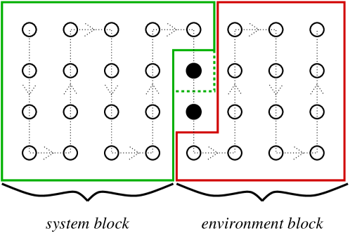
Figure 14: Superblock scheme for a two-dimensional lattice.

Recently, a variational scheme related to the DMRG and based on a tensor-based generalization of matrix product states has been argued to provide a better Verstraete and Cirac (unpublished) representation of two-dimensional wave functions. While the prelimary calculations look promising, the usefulness of this scheme in practice relative to the existent DMRG algorithms has not yet been explored.

5.4.2 Momentum-Space DMRG

Another approach to treating higher dimensional systems has been to work with a momentum-space formulation of a local Hamiltonian such as the Hubbard model. The Hamiltonian of the Hubbard model in momentum space reads

$$H=\sum_{k\sigma}\varepsilon_{k}\;c^{\dagger}_{k\sigma}c^{\phantom{\dagger}}_{k\sigma}+\frac{U}{N}\sum_{pkq}c^{\dagger}_{p-q\uparrow}c^{\dagger}_{k+q\downarrow}c^{\phantom{\dagger}}_{k\downarrow}c^{\phantom{\dagger}}_{p\uparrow}\;,$$ (108)

where $c^{\dagger}_{k\sigma}=1/\sqrt{N}\;\sum_{\ell}e^{ik\ell}c^{\dagger}_{\ell\sigma}$ is the Fourier-transformed electron creation operator and $N$ is the number of lattice sites. DMRG methods were first applied to this Hamiltonian by White in 1993 in unpublished work White (1993b) and subsequently independently implemented by Xiang with some additional algorithmic improvements Xiang (1996).

The basic idea is to carry out the standard finite-system DMRG algorithm (see Sec. 4.3.2) using the single-particle momenta as lattice points. The motivation for treating the momentum-space model is that all information about the dimensionality and lattice structure in Eq. (108) is contained in the first term which is diagonal. Therefore, the hope is to avoid the drastic loss in accuracy with dimension present in the real-space DMRG. The momentum-space basis is also a natural starting point for treating low-energy excitations relative to the filled Fermi sea. In addition, unlike in the real-space algorithm, it is easy to preserve and take advantage of the translational symmetry of the system, which translates to the conservation of total momentum in Hamiltonian (108). This can be used both to reduce the dimension of the Hilbert space in the diagonalization step and to calculate momentum-dependent observables. The disadvantage of the momentum-space formulation lies in the fact that the interaction term, the second term in Eq. (108), is highly non-local, which leads to both technical and fundamental problems.

There are three significant technical problems: the first is that, unlike for a short-range interactions like those in the Hubbard model in real space, there are formally a large number of terms in the interaction; in this case $N^{3}$. The impact of this problem can be reduced by factorizing the interacting into sums of terms that are internal to one block. As shown in Ref. Xiang (1996), this reduces the number of terms linking the parts of a two-part system to $6N$. Second, as in the two-dimensional algorithm described above, it is not possible to carry out the infinite-system algorithm to build up the lattice due to the lack of reflection symmetry at each step. However, a similar problem is present in the simplest variant of the real-space DMRG for two dimensions, as discussed in Sec. 5.4.1; some of the same techniques can be used here, such as taking a null environment block (equivalent to the Wilson procedure) or taking a small number of exactly treated sites as the environment. Third, it is not immediately clear how to order the momentum sites optimally in the DMRG algorithm because the interaction term links all sites with the same amplitude. Orderings in which momenta that are a similar distance from the Fermi surface are grouped together seem to be favorable Nishimoto et al. (2002); Legeza et al. (2003a), but the issue is still being explored Legeza and Sólyom (2003a). This problem also occurs in the DMRG treatment of other nonlocal Hamiltonians such as those obtained in quantum chemistry; see Sec. 6.4.

The crucial issue in the usability of the momentum-space DMRG is the convergence of the method, especially as compared to the real-space DMRG applied to similar systems. In particular, it is clear that the momentum-space DMRG becomes exact in the limit of weak interaction $U/t$ because Hamiltonian (108) becomes diagonal Xiang (1996). In contrast, the real-space DMRG becomes exact for the Hubbard model in the atomic limit $t\to 0$, but not directly in the strong-coupling limit $U/t\to\infty$. Therefore, for a given dimensionality, there is some interaction strength at which the momentum-space DMRG becomes more accurate than the real-space DMRG for the same lattice with the same boundary conditions. This occurs at approximately $U/t=8$ for a $4\times 4$ lattice Xiang (1996); Nishimoto et al. (2002). A comparison of the convergence for one- and two-dimensional lattices shows that comparable accuracy is attained when the ratio of the interaction to the bandwidth $U/W$ is approximately the same, with some additional small loss of accuracy with dimension Nishimoto et al. (2002).

6 Recent Developments in the DMRG

6.1 Classical Transfer Matrices

In contrast to interacting quantum systems, the ground state of a discrete classical model such as the Ising model can be trivially obtained: it is the behavior at finite temperature, characterized for instance by continuous phase transitions, that is interesting. The DMRG algorithm is powerful technique for obtaining approximate but very accurate information about the extremal eigenstates of an operator that operates on many-body Hilbert space composed of the direct products of the Hilbert spaces of its component systems. Transfer matrices for a classical systems have such properties and can be used to obtain thermodynamic properties. Therefore, a DMRG treatment of suitable transfer matrices, called the Transfer Matrix Renormalization Group (TMRG) can be used to calculate the thermodynamic properties of a classical system Nishino (1995). In addition, there is a well-known correspondence between a $d$-dimensional quantum and a $(d+1)$-dimensional classical system which makes it possible to calculate the thermodynamic properties of some quantum system, as will be discussed in Sec. 6.2.

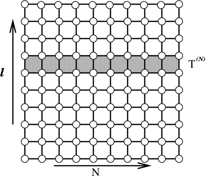
Figure 15: Schematic depiction of the finite row transfer matrix $T^{(N)}$ for the two-dimensional Ising model. Open boundary condition are applied in the $N$ direction and periodic boundary conditions in the $\ell$ direction, which is taken to become infinite.

Consider the two-dimensional Ising model with cylinder geometry so that $\ell$ ranges from 1 to $L$ with PBC and $n$ ranges from 1 to $N$ with OBC (see Fig. 15). The energy between nearest neighbors $i$ and $j$ is $-Js_{i}s_{j}$ where $s_{i}=\pm 1$ is an Ising spin variable. The symmetrical row transfer matrix in the $\ell$ direction can then be written as

$$T^{(N)}({\bf s}^{\prime}|{\bf s})=\exp\left(\frac{K}{2}s_{1}s^{\prime}_{1}\right)\left\{\prod_{n=1}^{N-1}W(s^{\prime}_{i}s^{\prime}_{n+1}|s_{i}s_{n+1})\right\}\exp\left(\frac{K}{2}s_{N}s^{\prime}_{N}\right)$$ (109)

where $\bf s=(s_{1},\ldots,s_{N})$ designates a vector of Ising spins, $K=J/k_{B}T$ is the dimensionless coupling, and

$$W(s^{\prime}_{i}s^{\prime}_{n+1}|s_{n}s_{n+1})=\exp\left[\frac{K}{2}(s^{\prime}_{n}s_{n}+s_{n}s_{n+1}+s^{\prime}_{n+1}s^{\prime}_{n}+s_{n+1}s^{\prime}_{n+1})\right]$$ (110)

is the Boltzmann weight connecting sites around a plaquette of four nearest neighbors. This matrix has dimension $2^{N}$ and is the object that will be treated with DMRG methods.

The thermodynamic properties can be derived from the partition function $Z$, which can be written in terms of the row transfer matrix as

$$Z={\rm Tr}\;\rho={\rm Tr}\;(T^{(N)})^{L}=\sum_{\alpha}(\lambda_{\alpha})^{L}\;$$ (111)

where the $\lambda_{\alpha}$ are the eigenvalues of $T^{(N)}$. (We assume that $T^{(N)}$ is diagonalizable and has positive semi-definite eigenvalues.) The trick in calculating $Z$ with a method that can accurately approximate the extremal eigenvalues of a finite sparse matrix such as the DMRG or iterative diagonalization is the take the limit $L\to\infty$, keeping $N$ finite, i.e., to make the lattice infinite in one direction only. The partition function can then be approximated as $Z\simeq\lambda_{1}^{L}$, where $\lambda_{1}$ is the largest eigenvalue of $T^{(N)}$. The (unnormalized) density matrix is given by $\rho=\lambda^{L}\;|\lambda_{1}\rangle\langle\lambda_{1}|$ where $|\lambda_{1}\rangle$ is the corresponding eigenvector.

In order to apply the DMRG method, the system, i.e., $T^{(N)}$, must be divided into two parts. If this is done at site $M$, $T^{(N)}$ can be written

$$T^{(N)}({\bf s^{\prime}}|{\bf s})=T_{L}({\bf s^{\prime}_{L}}|{\bf s_{L}})W(s_{M}^{\prime}s_{M+1}^{\prime}|s_{M}s_{M+1})T_{R}({\bf s^{\prime}_{R}}|{\bf s_{R}})\;$$ (112)

where

$$T_{L}({\bf s^{\prime}_{L}}|{\bf s_{L}})=\exp\left(\frac{K}{2}s^{\prime}_{1}s_{1}\right)\prod_{n=1}^{M-1}W(s^{\prime}_{i}s^{\prime}_{n+1}|s_{n}s_{n+1})$$ (113)

is the transfer matrix for the left half-row ${\bf s_{L}}=(s1,\ldots,s_{M})$ and $T_{R}({\bf s^{\prime}_{R}}|{\bf s_{R}})$ is defined analogously for the right half-row. The equivalent of the reduced density matrix used in the original DMRG is the left density submatrix defined as

$$\rho_{L}({\bf s}^{\prime}_{L}|{\bf s}_{L})=\sum_{{\bf s}_{R}}\rho({\bf s}^{\prime}_{L}\,{\bf s}_{R}|\,{\bf s}_{L}\,{\bf s}_{R})$$ (114)

(or the right density submatrix $\rho_{R}$, defined analogously). More than one eigenvalue of $\rho_{L}$ is important in the $L\to\infty$ limit, unlike the eigenvalues of $\rho$, but the eigenvalues generally decay rapidly, almost exponentially Baxter (1982); Peschel et al. (1999b) when the correlation length is finite. The partition function

$$\tilde{Z}=\sum_{i=1}^{m}\omega_{i}^{2}\;,$$ (115)

where the $\omega_{i}^{2}$ are the eigenvalues of $\rho_{L}$, for the partial system is bounded from above by the full partition function $Z$, and the difference becomes small when $m$ becomes large, or when the the eigenvalues $\omega_{i}^{2}$ fall off sufficiently rapidly.

The DMRG procedure is analogous to that for the quantum system, using iterative diagonalization to obtain the largest eigenstate of $T^{(N)}$ rather than the ground state of $H$ as for quantum systems. At each step, the local transfer matrix for a single plaquette $T^{(N)}$ is added to the finite lattice instead of a quantum site. As for the quantum system, the system can be built up to a given row length using the infinite-system algorithm, and then finite-system sweeps can be carried out until convergence is reached. One major difference in terms of efficiency compared with the calculation for the quantum algorithm is that there are no conserved quantum numbers, reducing the maximum number of states $m$ that can be kept for a given amount of numerical effort.

While all thermodynamic quantities can, in principle, be calculated by taking numerical derivatives of the free energy per site $f=-k_{B}T\ln Z/N\approx k_{B}T\ln\tilde{\lambda}_{1}$ (where $\tilde{\lambda}_{1}$ is the variational approximation to $\lambda_{1}$ obtained from the DMRG), second derivatives needed to obtain the susceptibility or specific heat are numerically unstable and it is better to use the first derivative of the energy per site, which can be calculated using matrix elements such as $\langle\lambda_{1}|s_{i}s_{j}|\lambda\rangle$, which, of course, also yield the short-range spin correlations. The correlation length $\xi$ can be calculated from the short-range spin correlations if they are small, or directly using $\xi=1/\ln{\rm Re}(\lambda_{2}/\lambda_{1})$, where $\lambda_{2}$ is the second-largest eigenvalue.

Applications of the TMRG for classical row transfer matrices include the two-dimensional Ising model Nishino (1995), the spin-3/2 Ising model Tsushima et al. (1997), wetting phenomena Carlon and Drzewiński (1997, 1998), the $q$-state Potts model Igloi and Carlon (1999), the $q$-state Potts model with random exchange Carlon et al. (1999), the 19-vertex model Honda and Horiguchi (1997), and the three-state chiral clock model Sato and Sasaki (2000). For a more extensive recent survey, see Ref. Schollwöck (2005).

It is also possible to treat Baxter’s corner transfer matrices Baxter (1968, 1982) using the DMRG, leading to the so-called Corner Transfer Matrix Renormalization Group (CTMRG) Nishino and Okunishi (1997). Since corner transfer matrices break up a two-dimensional square lattice into quadrants, the partition function is given by the fourth power of the corner transfer matrix

$$Z^{(2N-1)}={\rm Tr}\,\rho_{c}\approx{\rm Tr}\left(C^{(N)}\right)^{4}=\sum_{\nu=1}^{m}\alpha_{\nu}^{4}\;,$$ (116)

and converges variationally to the exact partition function in the thermodynamic limit and as the number of states kept $m$ becomes sufficiently large. Here the corner transfer matrix is defined as

$$C^{(N)}=\sum_{\{s\}}\prod_{\langle ijkl\rangle}W(s_{i}\,s_{j}\,|\,s_{k}\,s_{l})$$ (117)

and $\alpha_{v}$ are its (largest) eigenvalues. Baxter calculated the free energy per site in the $N\rightarrow\infty$ limit variationally Baxter (1968). Okunishi pointed out that Baxter’s treatment is essentially the infinite-system method of the DMRG Okunishi (Thesis (jap. version); Nishino and Okunishi formulated a numerical DMRG algorithm based on these ideas, the CTMRG Nishino and Okunishi (1997). It has the advantage that the eigenvalues of $C^{(N)}$ can be found without diagonalizing a large sparse matrix. The CTMRG has been used to find the critical exponents of the two-dimensional Ising model to high precision Nishino and Okunishi (1997), to investigate the spin-3/2 Ising model Tsushima and Horiguchi (1998) and a 7-configuration vertex model Takasaki et al. (2001), and to study models of two-dimensional self-avoiding walks Foster and Pinettes (2003a, b). Efforts are underway to generalize CTMRG-like algorithms to three-dimensional lattices Nishino and Okunishi (1998).

6.2 Finite Temperature

6.2.1 Low Temperature Method

In the original formulation of the DMRG White (1993a), it was clear that a system in a mixed state could the treated within the DMRG simply by obtaining excited states of the superblock in addition to the ground state and by including them in the system block density matrix:

$$\rho_{ii^{\prime}}=\sum_{\alpha}P_{\alpha}\sum_{j}\psi^{\alpha}_{ij}\psi^{\alpha\;*}_{i^{\prime}j}\;,$$ (118)

where the weight $P_{\alpha}\geq 0$, $\sum_{\alpha}P_{\alpha}=1$, and the $|\psi^{\alpha}\rangle$ are target states. For a system at finite temperature, the natural choice of the weight $P_{\alpha}$ might seem to be the Boltzmann weight $P_{\alpha}=e^{-\beta E_{\alpha}}$. Moukouri and Caron Moukouri and Caron (1996) pointed out, however, that $P_{\alpha}$ is only used to form the basis of the system block and does not enter into the calculation of expectation values directly. They found that it is more efficient to target a moderate number $M$ (typically 10 to 30) of superblock states and weight them equally, i.e., choose $P_{\alpha}=1/M$. In order to calculate thermodynamic properties, they form the superblock configuration shown in Fig. 16 in which the number of states kept in each block is sufficiently small so that a complete diagonalization can be carried out. The thermodynamical expectation value of an operator $A$ is then approximated by the Boltzmann sum

$$\langle A\rangle=\sum_{\gamma}e^{-\beta E_{\gamma}}\langle\psi^{\gamma}_{BB}|A|\psi^{\gamma}_{BB}\rangle\;,$$ (119)

where the set of eigenstates $E_{\gamma}$ is approximate and incomplete. The assumption is that the truncated basis of $\bar{H}_{B}$ gives an adequate description of the states in the Boltzmann sum even if they are not included as target states. This approximation is clearly better in the low-temperature regime and most likely breaks down at moderately high temperature. However, it has the advantage that it is a straightforward extension of the ground-state DMRG and therefore can treat the same systems, albeit with a somewhat higher computational cost. This method has been applied to $S=1/2$ and $S=3/2$ Heisenberg chains Moukouri and Caron (1996) and to an $S=1$ model for Y₂BaNiO₅ Batista et al. (1998); Hallberg et al. (1999).

Figure 16: Superblock configuration consisting of two truncated blocks.

6.2.2 Transfer Matrix Method

The correspondence between two-dimensional classical systems and one-dimensional quantum systems at finite temperature has led to the application of TMRG techniques to quantum transfer matrices Bursill et al. (1996); Wang and Xiang (1997); Shibata (1997a, 2003). In particular, taking the transfer matrix in the spatial direction leads to a method in which the system is at finite temperature, but in the thermodynamic limit. In order to formulate the quantum system as a two-dimensional classical lattice model, the partition function is discretized in the imaginary time or temperature direction using a Trotter-Suzuki (checkerboard) decomposition

$$Z={\rm Tr}\;e^{-\beta H}={\rm Tr}(e^{-\Delta\tau H_{\rm odd}}e^{-\Delta\tau H_{\rm even}})^{M/2}+{\cal O}(\Delta\tau^{2})\;,$$ (120)

where $\Delta\tau=\beta/2M$ is the imaginary time step,

$$H_{\rm odd}=\sum_{\ell=1}^{L-1}h_{2\ell-1,2\ell}\ \ \ \mbox{and}\ \ \ H_{\rm even}=\sum_{\ell=1}^{L-1}h_{2\ell,2\ell+1}$$

with $h_{\ell,\ell+1}$ being the Hamiltonian terms linking site $\ell$ with site $\ell+1$. (We assume that $H=H_{\rm odd}+H_{\rm even}$ contains only nearest-neighbor interactions.) The error is due to neglecting the commutator in factorizing the exponential. At this point a complete set of states $|\sigma^{j}_{\ell}\rangle$ is inserted at every point in space $\ell$ and imaginary time $j$ so that the partition function can be written as a discretized path integral

$$Z_{M}={\rm Tr}_{\{\sigma^{j}_{\ell}\}}\,\prod_{\ell=1}^{L/2}\,\prod_{j=1}^{M}\;\langle\sigma^{2j+1}_{2\ell-1}\;\sigma^{2j+1}_{2\ell}|e^{-\Delta\tau h_{2\ell-1,2\ell}}|\sigma^{2j}_{2\ell-1}\;\sigma^{2j}_{2\ell}\;\rangle$$

$$\hskip 108.12054pt\langle\sigma^{2j}_{2\ell}\;\sigma^{2j}_{2\ell+1}|e^{-\Delta\tau h_{2\ell,2\ell+1}}|\sigma^{2j-1}_{2\ell}\;\sigma^{2j-1}_{2\ell+1}\;\rangle\;.$$ (121)

The resulting lattice in space and imaginary time is shown schematically in Fig. 17. Note that the finite lattice treated with the TMRG is in the imaginary-time direction where the boundary conditions are periodic. By defining local transfer matrices on a plaquette as

$$\tau(\sigma\sigma|\sigma\sigma)\equiv\langle|e^{-\Delta\tau h_{\ell,\ell+1}}|\rangle\;,$$ (122)

the transfer matrices in the spatial direction for odd and even sites can be written as

$$T_{\rm odd}=\tau_{1,2}\tau_{3,4}\cdots\tau_{2M-1,2M}$$

and

$$T_{\rm even}=\tau_{2,3}\tau_{4,5}\cdots\tau_{2M,1}\;,$$

and the partition function for a finite discretization as

$$Z^{\infty}_{M}=\lim_{L\rightarrow\infty}{\rm Tr}\left(T_{\rm odd}T_{\rm even}\right)^{L/2}\;.$$ (123)

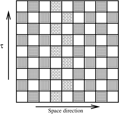
Figure 17: Checkerboard decomposition of the partition function. The quantum transfer matrix in the spacial direction is indicated by the region of differently marked squares.

As in the row-transfer TMRG for classical systems, the free energy per site is related to the largest eigenvalue of the transfer matrix, $\lambda_{1}$,

$$f_{M}=-\frac{k_{B}T}{2}\ln\lambda_{1}\;,$$ (124)

DMRG methods are used to obtain $\lambda_{1}$. The procedure is a direct adaptation of that for the classical case, except that:

• The detailed expressions for the transfer matrix are complicated by the checkerboard decomposition – the local transfer matrices only operate on the filled squares of the checkerboard, and the transfer matrix repeats itself after two rows rather than every row.

• Since the total transfer matrix is given by $T^{(M)}=T_{\rm odd}T_{\rm even}$ and since the commutator $[T_{\rm odd},T_{\rm even}]\neq 0$ in general, $T^{(M)}$ is not necessarily symmetric. However, the largest eigenvalue is real for physical cases, and a stable iterative diagonalization is possible, for example, with the Arnoldi or unsymmetrical Lanczos methods (see e.g. Ref. Bai et al. (2000)) with additional re(bi)orthogonalization. The left and right eigenvectors $\langle\psi_{L}|$ and $|\psi_{R}\rangle$ can thus be calculated and are most conveniently chosen to be biorthogonal $\langle\psi_{L}|\psi_{R}\rangle=0$.

• Conserved quantum numbers in the system Hamiltonian lead to corresponding conserved quantities in the transfer matrix, which can be used to reduce the dimension of the space treated in the iterative diagonalization.

• In order to perform basis reduction, the reduced density matrix $\rho={\rm Tr}_{e}|\psi_{R}\rangle\langle\psi_{L}|$, where the trace is over the basis of the environment block, is used. This in general unsymmetric matrix must be carefully diagonalized, taking into account numerical problems such as the appearance of spurious complex conjugate pairs of eigenvalues and the loss of biorthogonality Wang and Xiang (1997).

As in the classical case, the infinite-system algorithm followed by a number of finite-system sweeps can be carried out until convergence is attained. Since we are treating the infinite-system limit of the quantum transfer matrix in the spatial direction, the lattice size corresponds to the number of imaginary time steps taken, and the temperature $\beta=1/k_{B}T=M\Delta\tau$. Therefore, it takes more numerical effort to reach a lower temperature and the method should be numerically exact at high temperature. Since there is a systematic error associated with the finite imaginary time step $\Delta\tau$, the extrapolation $\Delta\tau\to 0$ should be carried out to obtain (numerically) exact results. Thermodynamic quantities can be calculated as numerical derivatives of the free energy, or can be formed a calculation of the local energy, as in the classical case. Dynamical quantities for quantum systems, as discussed in Sec. 2.4 can be calculated at finite temperature with two caveats. First, only spatially local or at most short-range expectation values can be easily calculated because the transfer matrix only contains spatial information at a range of two sites. Second, the dynamical information in the imaginary time direction can be obtained directly from the calculation of the appropriate correlation functions on the imaginary-time lattice. However, the experimentally relevant dependence is on real frequency. The analytic continuation of imaginary-time data to read frequencies occurs via an inverse Laplace transform, which is an ill-posed problem. This issue of how to perform such an analytic continuation numerically and what the limitations are has been extensively investigated in the context of quantum Monte Carlo calculations; the Maximum Entropy method is the most used technique Silver et al. (1990).

The quantum TMRG has been applied to calculate the thermodynamic properties of a number of systems, including spin chins Shibata (1997b); Wang and Xiang (1997); Xiang (1998), spin chains with frustration Maisinger and Schollwöck (1998); Klümper et al. (1999, 2000), the one-dimensional $t$-$J$ model Ammon et al. (1999); Sirker and Klümper (2002a, b), the one-dimensional Kondo lattice model Shibata et al. (1998); Shibata and Tsunetsugu (1999a), and a spin-orbit model Sirker and Khaliullin (2003). Dynamical quantities have been calculated for anisotropic spin chains Naef et al. (1999), the one-dimensional Kondo model Mutou et al. (1998); Shibata and Tsunetsugu (1999b), and the nuclear spin relaxation rate in two-leg spin ladders Naef and Wang (2000).

6.3 Dynamics

As discussed in Sec. 2.4, the calculation of dynamical quantities is a demanding task. In order to obtain the dynamical correlation function

$$G({\bf k},\omega)=\langle\psi_{0}|A^{\dagger}_{\bf k}(\omega+i\eta-H)^{-1}A_{\bf k}|\psi_{0}\rangle\;,$$ (125)

a ground state calculation is not sufficient. It is necessary to obtain additional states, which in the DMRG must be included in the density matrix as target states. The methods vary in which states are targeted, but the state $A_{\bf k}|\psi_{0}\rangle$ must be targeted in addition to the ground state in all methods.

The first approach to the calculation of dynamical properties using the DMRG that was developed is the Lanczos vector method Hallberg (1995). In this approach, the sequence of Lanczos vectors which span the Krylov subspace

$$|\psi_{0}\rangle,\ A_{\bf k}|\psi_{0}\rangle,\ HA_{\bf k}|\psi_{0}\rangle,\ H^{2}A_{\bf k}|\psi_{0}\rangle,\;\ldots$$ (126)

are targeted. In this way, the Lanczos coefficients can be obtained and the spectral function can be calculated using the continued-fraction representation, Eq. (33). This provides the spectral function for the full range of $\omega$ in one run. Usually, one restricts the target vectors to approximately the first 10 vectors of the Krylov subspace; otherwise, the DMRG run would become too expensive because the number of states kept would have to be increased in order to obtain the low-lying states sufficiently accurately. However, this number of states is generally not sufficient to reach convergence in the continued fraction expansion. In order to overcome this problem, the Lanczos recursion is continued using vectors that are not targeted in the density matrix. However, the additional Lanczos vectors are represented in a basis of density-matrix eigenvectors which have not been adapted for these vectors. This could lead to uncontrolled errors.

An alternative approach which overcomes this problem is the correction vector method Kühner and White (1999). It is based on the correction vector method for iterative diagonalization Soos and Ramasesha (1989) discussed in Sec. 2.4.2 and was further developed and successfully applied in Ref. Raas et al. (2004). In this approach, the target vectors

$$|\psi_{0}\rangle,\ A_{\bf k}|\psi_{0}\rangle,\ (\omega+i\eta-H)^{-1}A_{\bf k}|\psi_{0}\rangle$$ (127)

are included in the density matrix. The method is more accurate but more costly than the Lanczos vector method, since for each value of $\omega$ a separate run must be performed.

The direct inversion of the resolvent operator can be carried out with a procedure such as the conjugate gradient method, but this procedure is computationally costly and can be unstable. (These problems can be minimized by a better choice of methods for the inversion Raas et al. (2004).) A variant of this method was introduced by Jeckelmann Jeckelmann (2002) which leads to a more efficient and stable method. The basic observation is that the correction vector minimizes the functional

$$W_{A,\eta}(\omega,\psi)=\langle\psi|(E_{0}+\omega-H)^{2}+\eta^{2})|\psi\rangle\,+\,\eta\langle\psi_{0}|A|\psi\rangle\,+\,\eta\langle\psi|A|\psi_{0}\rangle\;.$$ (128)

The spectral weight is then given by

$$W_{A_{\bf k},\eta}(\omega,\psi_{\rm min})=-\pi\eta\,{\rm Im}\,G({\bf k},\omega)\;.$$ (129)

In the calculation, the correction vector is split up into imaginary and real parts

$$(\omega+i\eta-H)^{-1}A_{\bf k}|\psi_{0}\rangle=|X_{A}(\omega+i\eta)\rangle+i|Y_{A}(\omega+i\eta)\rangle\;.$$ (130)

The target-states used in this approach are

$$|\psi_{0}\rangle,\,A_{\bf k}|\psi_{0}\rangle,\,|X_{A}(\omega+i\eta)\rangle,\,|Y_{A}(\omega+i\eta)\rangle.$$ (131)

The DMRG procedure can be formulated so that it simultaneously minimizes the ground-state energy and provides the minimum of the functional $W_{A,\eta}(\omega,\psi)$ Jeckelmann (2002); Benthien (2005).

Using this approach, several investigations have been performed. In the following we will outline the procedure by outlining the calculation of the single-particle spectral weight for the Hubbard chain Benthien et al. (2004). The 1D Hubbard model with open boundary conditions has the Hamiltonian

$$H=-t\sum^{L-1}_{\ell=1,\sigma}\left(c^{\dagger}_{\ell,\sigma}c^{\phantom{\dagger}}_{\ell+1,\sigma}+c^{\dagger}_{\ell+1,\sigma}c^{\phantom{\dagger}}_{\ell,\sigma}\right)+U\sum^{L}_{\ell=1}n_{\ell,\uparrow}n_{\ell,\downarrow}\;.$$ (132)

The single-particle spectral weight for holes (as obtained in photoemission experiments) is defined by

$$A(k,\omega)=\frac{1}{\pi}\,{\rm Im}\,\langle\psi_{0}|\;c^{\dagger}_{k,\sigma}\;\frac{1}{H+\omega-E_{0}+i\eta}\;c^{\phantom{\dagger}}_{k,\sigma}\;|\psi_{0}\rangle$$ (133)

where

$$c^{\phantom{\dagger}}_{k,\sigma}\,=\,\frac{1}{\sqrt{L}}\sum_{\ell}e^{ik\ell}\,c^{\phantom{\dagger}}_{\ell,\sigma}\;.$$ (134)

This definition of $c^{\phantom{\dagger}}_{k,\sigma}$ is problematic because the Fourier transform used is only defined for periodic boundary conditions, while a system with open boundary conditions is generally treated by the DMRG for reasons of efficiency (see Sec. 4.2). The solution is to carry out the transform using “particle-in-a-box” eigenstates,

$$c^{\phantom{\dagger}}_{k,\sigma}=\sqrt{\frac{2}{L+1}}\sum_{\ell}\;\sin(k\ell)\;c^{\phantom{\dagger}}_{\ell,\sigma}\;.$$ (135)

A comparison of the results obtained with the analytic and exact Bethe-Ansatz method shows excellent agreement. Thus, it is possible to obtain momentum-dependent dynamical quantities using open boundary conditions, for which the DMRG works best. For this model, relatively large system sizes can be reached (about 200 sites for a Hubbard chain on present-day desktop PCs).

6.4 Quantum Chemistry

Quantum chemical or ab initio treatments of a solid can be cast into the form of a lattice Hamiltonian once a suitable single-particle basis of $N$ orbitals has been chosen. The generic form of the Hamiltonian is then

$$H=\sum_{i,j,\sigma}t_{ij}c_{i\sigma}^{\dagger}c^{\phantom{\dagger}}_{j\sigma}+\frac{1}{2}\sum_{i,j,k,l}G_{ijkl}\sum_{\sigma,\sigma^{\prime}}c_{i\sigma}^{\dagger}c_{j\sigma^{\prime}}^{\dagger}c^{\phantom{\dagger}}_{k\sigma^{\prime}}c^{\phantom{\dagger}}_{l\sigma}.$$ (136)

where $c^{\dagger}_{i\sigma}$ creates an electron in molecular orbital $i$, $t_{ij}$ is the single-electron integral of molecular orbitals $i$ and $j$, and $G_{ijkl}$ is the two-electron integral (Coulomb repulsion) White and Martin (1998). This Hamiltonian can be treated using the iterative diagonalization methods described in Sec. 2.3; in quantum chemistry nomenclature, this is termed a “full Configuration-Interaction” (full-CI) calculation. Since the Hamiltonian (136) has a form that is similar to but more general than the Hubbard model in momentum-space (108), DMRG methods that are similar to those used in the momentum-space DMRG can be applied and similar technical problems crop up. In particular, the molecular orbitals take the role of the single-particle momenta with the difference that there is no momentum conservation. A one-dimensional path is chosen in this space of molecular orbitals and similar problems occur in the initial buildup of the lattice. Both the single-electron term and the two-electron term are non-diagonal in general. The two-electron term can be factorized into sums of terms internal to a block as in the momentum-space algorithm; however, the minimum number of terms scales as $N^{2}$ rather than $N$ because of the absence of momentum conservation White and Martin (1998). The computational cost of the algorithm scales as $(N^{4}m^{2}+N^{3}m^{3})$, where the first term comes from the formation of the necessary operators as a site is added to a block and the second is due to multiplication of the ${\cal O}(N^{2})$ representations of operators on a block, which comes about either when performing a change of basis on the representation of an operator, or performing the multiplications necessary to form the product $H|\psi\rangle$ needed for the iterative diagonalization White and Martin (1998). (Each operation is repeated ${\cal O}(N)$ times in the finite-system algorithm.)

As in the momentum-space algorithm, which ordering of the sites, i.e., the molecular orbitals, is optimal is not clear. It seems that the ordering can strongly effect both the performance (i.e., how many finite-system steps are required to reach convergence) and the ultimate accuracy of the result Legeza and Sólyom (2003b); ris (Private communication by Jörg Rissler.). In particular, some orderings can lead to a convergence to higher-lying metastable states. Unfortunately, a general method to find a globally optimal ordering has not yet been found. The simplest possibility is to use information from the Hartree-Fock energy and occupation of the orbitals to choose the ordering, typically keeping partially occupied orbitals near each other in the center of the chain White and Martin (1998); Daul et al. (2000); Mistrushenkov et al. (2001, 2003). Another approach is to use information from the single-particle matrix elements $t_{ij}$. In Ref. Chan and Head-Gordon (2002) the symmetric reverse Cuthill-Mckee reordering, which attempts to make $t_{ij}$ as band-diagonal as possible, was shown to lead to faster convergence in $m$ and the number of finite-system sweeps as compared to Hartree-Fock ordering. Improvement was also obtained by optimizing the ordering using the Fock term which contains contributions from both $t_{ij}$ and parts of the interaction $V_{ijkl}$ Legeza et al. (2003b). Ideas from Quantum Information Theory also seem to be important: Legeza and Sólyom Legeza and Sólyom (2003a) have shown that the profile along the chain of the entanglement entropy between single sites and the rest of the system is important. In particular, orderings which lead to fast convergence tend to have sites with high entanglement entropy grouped together near the center of the chain.

Another possibility to improve the quantum chemical algorithm is to change the choice of single-particle orbitals either by choosing a different set of single-particle orbitals at the outset or by performing a canonical transformation on the single-particle basis

$$\tilde{\phi}_{i}=\sum_{j}U_{ij}\phi_{j}$$

where $U_{ij}$ is unitary and $\phi_{i}$ and $\tilde{\phi}_{i}$ represent single-particle bases. Since such a transformation can change the range and topology of connections of both $t_{ij}$ and $V_{ijkl}$, the performance of the DMRG algorithm can be strongly affected. Daul et al. Daul et al. (2000) applied a procedure in which orbitals unoccupied at the Hartree-Fock level were localized, but did not find a significant improvement in the convergence as compared to standard Hartree-Fock orbitals for the HHeH molecule. White White (2002) applied a continuous sequence of canonical transformations related to the flow equation method Wegner (1994); Glazek and Wilson (1994) in order to reduce non-diagonal matrix elements. Calculations for the stretched water molecule as compared to full-CI calculations show promising results White (2002); this method remains to be further explored.

Thus far, the DMRG for quantum chemistry has been primarily applied to relatively small molecules in order to test and develop the method. Full-CI results carried out with the same basis set as the DMRG calculations have provided a useful benchmark for the DMRG method. In particular, the water molecule has been treated in the DZP basis with 8 electrons on 25 molecular orbitals which is small enough so that full-CI results are available White and Martin (1998); Daul et al. (2000); Chan and Head-Gordon (2002); Legeza et al. (2003a). Agreement with full-CI to within 0.004 mH (Hartree) is possible, keeping up to $m=900$ states Chan and Head-Gordon (2002); Legeza et al. (2003a). A TZ2P basis with 10 electrons on 41 orbitals, which is too large to treat with full-CI methods has also been treated with the DMRG, yielding an estimated accuracy of 0.005mH in the ground-state energy for $m=5000$, approximately a factor of three lower than the best coupled cluster method Chan and Head-Gordon (2003). The energy dissociation curves for N₂ Mistrushenkov et al. (2001) and H₂O Mistrushenkov et al. (2003), and excited states of the HHeH molecule Daul et al. (2000) and CH₂ Legeza et al. (2003a) have been calculated with good accuracy. For LiF, the ground and excited states and the dipole moment were calculated to relative accuracies of $10^{-9}$, $10^{-7}$, and $10^{-3}$, respectively, as compared to full-CI results near the avoided crossing associated with the ionic-neutral crossover of the bond Legeza et al. (2003b).

6.5 Time Evolution

As discussed in Sec. 2.5, the time evolution of a state in quantum mechanics is governed by the time-dependent Schrödinger-equation, Eq. (3), with the formal solution

$$|\psi(t)\rangle=e^{-iHt}\;|\psi(0)\rangle\;.$$ (137)

Typically, one is interested in the behavior of the system after a perturbation

$$H=H_{0}+H_{1}\;\Theta(t)$$

is switched on at $t=0$ or after an external operator

$$A^{\dagger}\;|\psi_{0}\rangle.$$

is applied. In order to calculate the time evolution of the system, one either has to integrate Eq. (3) directly or one has to find a suitable approximation for the time-evolution operator $\exp(-iHt)$. In the context of the DMRG, both approaches have been utilized. Recent developments are recapitulated in Ref. Schollwöck (unpublished).

In the direct integration approach, a Runge-Kutta integration Press et al. (1993) of the time evolution was carried out Cazalilla and Marston (2002). As pointed out in Ref. Luo et al. (2003), the main difficulty in calculating the time evolution using the DMRG is that the effective basis determined at the beginning of the time evolution is not able, in general, to represent the state well at later times because it covers a subspace of the system’s total Hilbert space which is not appropriate to properly represent the state at the next time step. As discussed in Refs. Manmana et al. (2005); Luo et al. (2003), it is possible that the representation of the time-dependent wave function very soon becomes quite bad. It is therefore necessary either to mix all time steps $|\psi(t_{i})\rangle$ into the density-matrix Luo et al. (2003); Schmitteckert (2004), or to adapt the density matrix during propagation. An approach for adaptive time evolution basing on the Trotter-Suzuki decomposition of the time-evolution operator was developed in Refs. Vidal (2004); White and Feiguin (2004); Daley et al. (2004). In this approach, the time-evolution operator is divided into two-site terms which can be applied to the two sites included exactly in a typical superblock-configuration. However, the method is restricted to systems with nearest-neighbor terms in the Hamiltonian only. A more general scheme to carry out the evolution through one time step that is closely related to exact techniques and is combined with an adaption scheme recently proposed by White Feiguin and White (unpublished) is presented in a second contribution of the authors in this volume, Ref. Manmana et al. (2005). In this approach, the time-evolution operator is expanded in a Lanczos basis in a similar manner to the time evolution approach used in the exact diagonalization scheme, as discussed in Sec. 2.5. By using the multi-target method discussed in Feiguin and White (unpublished); Manmana et al. (2005), it is possible to efficiently calculate the time evolution of systems which can be treated with the DMRG, even if the Hamiltonian contains terms connecting sites that are not nearest neighbors, e.g., on ladder systems. However, the how to carry out the targeting optimally is still under investigation and will be presented elsewhere Manmana et al. (in preparation).

Since it is possible to treat fairly large systems with the time-dependent DMRG, it is well-suited to investigate strongly correlated quantum systems out of equilibrium; such a tool was missing until now. The application of the DMRG to such systems opens up new possible applications to a variety of systems in the near future. For recent investigations using this method, see Refs. Schollwöck (unpublished); Manmana et al. (2005) and references therein. Note that it is also possible to use the time-dependent DMRG to investigate spectral quantities by directly calculating the Fourier transform of time-dependent correlation functions. This method should be faster than the DDMRG presented in Sec. 6.3 when a complete spectrum is required because information for a wide range of frequencies can be obtained in one DMRG run. However, it is likely that the DDMRG will still provide more accurate results for a given frequency $\omega$.

6.6 Matrix Product States

In the DMRG procedure, the state of the system block is changed in two steps: First, degrees of freedom are added to the system by adding a site (or other subsystem) to the system block, increasing the size of the basis

$$|\alpha\rangle_{\ell}\otimes|s_{\ell}\rangle\to|\beta^{\prime}_{\ell+1}\rangle\;.$$ (138)

Second, this expanded system is transformed to a new truncated basis (i.e., the eigenbasis of the density matrix with the largest eigenvalues).

$$|\beta_{\ell+1}\rangle=u^{\beta}_{\beta^{\prime}}|\beta^{\prime}_{\ell+1}\rangle$$ (139)

In fact, both steps can be combined into one transformation, as was done in the wave function transformation discussed in Sec. 5.3

$$|\beta_{\ell+1}\rangle=\sum_{s_{\ell},\alpha}A^{s}_{\beta\alpha}|\alpha_{\ell}\rangle\otimes|s_{\ell}\rangle\;.$$ (140)

For each state of the added site $s$, the matrix $A^{s}_{\beta\alpha}$ maps from the basis $\alpha_{\ell}$ describing a system block with $\ell$ sites to $\beta_{\ell+1}$, the truncated basis for a system block with $\ell+1$ sites; typically these bases are the same size. Since the other half of the system, i.e., the environment, is built up in a similar fashion (either symmetrically in the infinite-system algorithm or in a previous finite-system sweep), its basis can be described as a similar series of transformations. The DMRG wave function can then, in general, be written as a sum of such products, leading to the state Östlund and Rommer (1995)

$$|\psi_{\rm MP}\rangle=\sum_{\{s_{\ell}\}}{\rm Tr}\left\{\;A^{s_{1}}\,A^{s_{2}}\,A^{s_{3}}\ldots A^{s_{L}}\right\}|s_{1},s_{2},\ldots,s_{L}\rangle\;.$$ (141)

Here the $A^{s_{\ell}}$ are $m\times m$ matrices, except for $A_{1}$ and $A_{L}$ which are $m$-element vectors. (We assume that the same number $m$ states are retained at each step; generalization to a variable number of states is straightforward.) The trace is carried out over the set of coordinates of the added sites. Generally, a normalization

$$\sum_{\{s_{\ell}\}}A^{s_{\ell}}(A^{s_{\ell}})^{\dagger}=\leavevmode\hbox{\small 1\normalsize\kern-3.30002pt1}$$ (142)

is chosen for the $A$-matrices. This is a special case of a matrix product state. The DMRG can be viewed as a particular variational calculation in the space of such states Östlund and Rommer (1995); Verstraete et al. (2004a). Note that a matrix product state for periodic boundary conditions can be formed if the vectors $A_{1}$ and $A_{L}$ are replaced by matrices. A translationally invariant state would then have all $A^{s_{\ell}}=A^{s}$ equal Verstraete et al. (2004a).

It is useful to consider matrix product states and their properties in more generality. In particular, any state can be described as a matrix product state if the dimension of the $A^{s_{\ell}}$ at each step is large enough. However, this is not useful in itself: the required dimension can, in principle, grow exponentially with the system size. Nonetheless, some states are very compactly described: the Neél state $|\uparrow\downarrow\uparrow\downarrow\uparrow\ldots\rangle$ can be trivially described using $1\times 1$ matrices and the Bell state $|\uparrow\uparrow\uparrow\ldots\rangle\pm|\downarrow\downarrow\downarrow\ldots\rangle$ using simple $2\times 2$ matrices. The valence-bond solid state for the spin-1 chain, which provides a qualitatively useful description of the ground state for the Heisenberg Hamiltonian and is the exact ground state of the Affleck-Kennedy-Lieb-Tasaki (AKLT) Hamiltonian Affleck et al. (1987, 1988), can be described as a matrix-product state with $m=2$.

For a matrix product state with a particular structure, the elements of the matrices play the role of variational parameters. The value of the parameters can, in general, be variationally optimized using a variety of methods. For example, the power method (see Sec. 2.3), in which the Hamiltonian is repeatedly applied to the variational state, $H^{n}|\psi_{\rm MP}\rangle$, imaginary time evolution, $e^{\Theta H}|\psi_{\rm MP}\rangle$, or iterative diagonalization methods such as the Lanczos method, all can be used. The DMRG algorithm is somewhat more complicated to formulate in detail in terms of matrix product states; see Ref. Verstraete et al. (2004a). Expectation values of a set of arbitrary operators residing on different sites can be evaluated directly in terms of matrix products if the relevant operators are expressed as $m^{2}$-dimensional operators and are inserted into the matrix product at the appropriate points Andersson et al. (1999).

This leads to the question of whether other algorithms based on matrix product states are better than the DMRG for particular systems. Recently, a number of such algorithms have been formulated, especially for systems and situations in which the DMRG either does not perform well or cannot be applied. In particular, the DMRG does not produce translationally invariant states, leading to poor convergence for one-dimensional systems with periodic boundary conditions. Verstraete, Porras, and Cirac Verstraete et al. (2004a) have formulated a variational algorithm that is closely related to the DMRG based on a translationally invariant matrix product state. In contrast to the matrix product state generated by the DMRG, their state has same degree of entanglement between all sites, including those spanning the boundary. The diagonalization of the superblock Hamiltonian used in the DMRG algorithm is replaced by the minimization of a more general functional and the sweeping back and forth in the finite system algorithm is replaced by sweeping in the positive or negative direction around the ring-like lattice. This algorithm apparently yields a convergence with the number of states kept $m$ for the Heisenberg chain with periodic boundary conditions that is comparable to that of the DMRG for a chain of the same length with open boundary conditions. However, the computational cost of the new algorithm is larger than the DMRG, order $m^{5}$ rather than order $m^{3}$ because sparseness of the matrix representations is lost, and implementations of comparable efficiency to current DMRG codes do not yet exist, so that the utility of the method for realistic systems remains to be determined.

Generalizations of matrix product states have been formulated which incorporate ancilla subspaces so that mixed states can be represented Verstraete et al. (2004b); Zwolak and Vidal (2004). Such states can be used to represent dissipative quantum or quantum systems at finite temperature. Starting with a completely mixed state corresponding to infinite temperature, imaginary time evolution with a Trotter-decomposed operator can be carried out to obtain a finite-temperature state Verstraete et al. (2004b); Zwolak and Vidal (2004). Such a state can then be further evolved in real time using the methods discussed in Sec. 6.5, yielding the time-dependent behavior of finite-temperature or dissipative systems. Since these methods have been proposed quite recently, they still await application to realistic systems.

Generalizations of matrix product states that are better suited to two-dimensional systems have also been proposed Verstraete and Cirac (unpublished). For a two-dimensional square lattice, such a state must represent the entanglement of a site to its four nearest neighbors. This can be done by inserting an ancilla space for each bond direction, leading to to a state that is represented by a product of rank-4 tensors. (Such tensor product states are related to corner transfer tensor states that have been considered for three-dimensional classical systems Nishino and Okunishi (1998).) In Ref. Verstraete and Cirac (unpublished), such a state is variationally optimized for the two-dimensional Heisenberg model with and without frustration using imaginary-time evolution, yielding promising variational results for bond dimensions (analogous to the number of states kept, $m$) of up to 4. However, since the algorithm seems to scale with a quite high power of $m$, its utility for realistic system remains to be explored.

As we have seen, recent developments in understanding the correspondence between the DMRG and matrix product states and in formulating algorithms based on matrix product states and their generalizations have opened up many exciting new possibilities in developing new numerical methods for interacting quantum systems.

6.7 Quantum Information and the DMRG

As discussed in Sec. 4.2, the basic approximation used to truncate the Hilbert space of the superblock in the DMRG is based on dividing it in two parts given that the superblock is in a pure state (in the simplest case). The accuracy of the approximation is intimately connected to the degree of entanglement between the two parts of the bipartite system, i.e., between the system block and the environment block. Such entanglement is in turn intimately connected with the mutual quantum information in the two subsystems. Recently, progress has been made in utilizing this connection between the DMRG and quantum information theory to improve the understanding of the behavior of errors within the DMRG, to minimize the error in the DMRG algorithm for a given computational cost, to improve extrapolation methods for calculated quantities, and to formulate improved variants of the DMRG algorithm.

A measure of mutual entanglement is the von Neumann or mutual quantum information entropy $S$, defined in Eq. (87). Since this quantity can be written as $-\sum_{\alpha}w_{\alpha}\log w_{\alpha}$, its behavior is a measure of the behavior of the eigenvalues of the density matrix $w_{\alpha}$. The von Neumann entropy and related quantities from quantum information theory can be used to analyze the behavior of the DMRG algorithms in a quantitative way and to reformulate and optimize the algorithms. In particular, Legeza et al. Legeza et al. (2003a) have formulated a scheme to vary the number of states kept $m$ dynamically according to a criterion based on keeping the truncation error, as measured by the weight of the discarded density-matrix eigenvalues, constant. The relationship between the truncation error, the von Neumann entropy, and the size of the complete Hilbert space was explored in Refs. Legeza and Sólyom (2003a) and Legeza and Sólyom (2004) for the Hubbard model in momentum space and for quantum chemistry. The Kholevo bound for the accessible information in a quantum channel,

$$\chi=S(\rho)-p_{\rm typ}\,S(\rho_{\rm typ})-(1-p_{\rm typ})\,S(\rho_{\rm atyp})\;,$$ (143)

where $\rho_{\rm typ}$ is the density matrix and $p_{\rm typ}$ the weight of the typical subspace, corresponding to the portion of states kept, and $\rho_{\rm atyp}$ the density matrix of the atypical subspace, corresponding to discarded states, was argued to be a good measure of the information loss due to truncation, and was used as a criterion for adjusting $m$ and as a means of extrapolating energies Legeza and Sólyom (2004). Considerations based on the von Neumann block entropy and the Kullback-Leibler entropy Kullback and Leibler (1951); Kullback (1959) have been used to investigate criteria for the optimal ordering of sites and to formulate a more efficient, dynamical procedure to build up the lattice in the quantum chemistry and momentum-space DMRG Legeza and Sólyom (2003a).

Another interesting issue is how the behavior of the von Neumann entropy depends on whether or not a system is critical. This has been investigated for one-dimensional XY, XXZ, and Heisenberg spin chains in Ref. Latorre et al. (2004). The results are that when the system is not at a quantum critical point, the von Neumann entropy $S_{L}$ for a particular chain length $L$ saturates when $L$ is of the size of the correlation length. For critical systems, $S_{L}$ is shown to grow logarithmically with $L$, an unbounded behavior, but with a growth that is much slower than the upper bound on the entropy, $S_{L}\sim L$. The authors argue that the prefactor of this logarithmic divergence depends only on the universality class of the critical point.

The connection between the DMRG and quantum information theory suggests that the DMRG algorithm could possibly be applicable to problems in quantum information theory such as how decoherence occurs in detail or what the bounds on the information transmitted in a noisy channel are, either through the direct simulation of model systems or through the use of insights gained from the analysis of the DMRG algorithm and its generalization using concepts from quantum information theory.

7 Conclusion and Outlook

In this tutorial, we have discussed a number of closely related numerical methods for investigating strongly interacting quantum many-body systems based on numerical diagonalization. The aim is to treat quantum lattice models, systems composed of sites, usually on a regular lattice, with a finite number of quantum mechanical states. The size of the Hilbert space of such a model grows exponentially with the number of sites, making treatment of sufficiently large lattices to scale to the thermodynamic limit difficult. The prototypical models considered here, such as the quantum Heisenberg model or the Hubbard model, originate as effective models for interacting electrons in a solid, but quantum lattice models can also come about in other physical systems such as atomic nuclei, arrays of trapped atoms, or, in general, through the discretization of a quantum field theory.

All methods discussed here are based on numerical diagonalization, with the NRG and the DMRG having an additional variational approximation in which the dimension of the Hilbert space treated numerically is systematically reduced. “Exact diagonalization” methods treat the entire Hilbert space of the finite lattice Hamiltonian, which can be restricted to particular symmetry sectors. “Complete diagonalization” uses standard algorithms whose cost scales as the cube of the dimension to obtain all eigenstates. Since at most Hilbert spaces dimension of order $10^{3}$, corresponding to very small lattice size, can be treated, the method is useful primarily for testing and for benchmarks for other methods. “Iterative diagonalization” can calculate extremal eigenstates for much larger Hilbert spaces, up to of order $10^{9}$, corresponding to system sizes of up to approximately 40 sites for the simpler quantum lattice models. This is done by using an iterative procedure to project the Hamiltonian onto a cleverly chosen subspace. While the method is formally variational, convergence to almost machine precision is attained for typical quantum lattice models. The methods has also been extended to efficiently calculate dynamical correlation functions, finite-temperature properties, and time evolution of a quantum system, properties that, in principle, depend on excited states. The ability of iterative diagonalization to provide results that are essentially exact for numerical purposes for a wide variety of properties with few restrictions on the type of Hamiltonian or lattice makes it an important standard tool. However, the restriction to moderate lattice sizes due to the exponential growth of the Hilbert space of quantum lattice models with system size limits its usefulness in extrapolating to the thermodynamic limit. The method is more useful for low-dimensional systems simply because the linear dimension is often the relevant parameter in such an extrapolation.

The numerical renormalization group is an iterative procedure in which a (“complete”) numerical diagonalization is combined with a truncation of the Hilbert space to lowest energy eigenstates and the addition of degrees of freedom by adding lattice sites. The numerical effort is linear in the system size when the number of states kept is held fixed. However, the approximation is only well-controlled for one-dimensional quantum lattice models with coupling between sites which fall off exponentially with position. Thus, the NRG is limited to systems that can be mapped onto such a model; these are primarily single-impurity models such as the Kondo model and the single-impurity Anderson model, including its generalization for the dynamical mean-field theory. The NRG is an extremely powerful method for such systems and can be used to calculate renormalization group flows, finite-temperature properties and dynamic quantities such as the impurity density of states.

The density matrix renormalization group generalizes the NRG by circumventing problems with the treatment of the wavefunction at the boundaries present in the NRG. This is done by embedding a NRG procedure in a larger lattice in which the diagonalization is carried out. The reduced density matrix of the renormalized subsystem corresponding to one or more states of the system is used to carry out the truncation of the basis in a way that can be shown to be optimal. The ability to choose the state or states of the system to which the truncated basis is adapted allows specialization of the algorithm for specific purposes, such as calculation of the ground state only or the ground state and low-lying excited states or other additional states. The freedom of choosing how to divide the system at each step leads to two classes of algorithms: the infinite-system algorithm in which the system grows by two sites at each step, and the finite-system algorithm in which the size of the system is kept fixed. While the infinite-system algorithm is useful in building up the system at the beginning of the procedure or in scaling directly to the infinite-system limit, use of the finite-system procedure leads to more accurate results in almost all cases.

Crucial to the applicability of the DMRG is how quickly the eigenvalues of the density matrix fall off; this determines the accuracy of the variational approximation and is intimately related to the entanglement of the parts of the system. For determination of ground-state properties, one-dimensional lattices with open boundary conditions can be most accurately treated. It is also favorable for the system to have a gap in one or more symmetry sectors of the spectrum, leading to a finite correlation length in the associated correlation function. Critical one-dimensional systems have behavior that is less favorable, in particular as the lattice size is increased, and two-dimensional systems require exponentially many states to be kept with lattice size in the worst case. Therefore, the DMRG has become an extremely powerful standard tool for the calculation of low-energy properties of short-range quantum lattice models in one-dimension and on coupled chains.

Adaptations of the finite-system algorithm to systems with long-range interactions such as the Hubbard model in momentum space and quantum chemical systems have been formulated. The momentum-space algorithm becomes more accurate as the coupling becomes weaker and its convergence only weakly dependent on dimension; however, it is not competitive with the real-space method for one-dimensional and coupled chain systems at moderate to large interaction strength. Application to models with longer-range interactions in real space corresponding to shorter-range interactions in momentum space should be promising to explore. The quantum chemical DMRG is competitive with other quantum chemical methods for small molecules, but more development to improve the performance of the algorithm must be done for it to be useful for a wider variety of quantum chemical problems.

Calculation of dynamical correlation functions using the DMRG can be carried out with adaptations of both methods used in iterative diagonalization, the continued fraction (Lanczos basis) method and the correction vector method. The latter method provides substantially more accurate information at a given frequency at the price of having to carry out a separate calculation at each frequency to be obtained. While some optimization of algorithm is probably possible, these techniques seem to be relatively mature, although they remain to be applied widely to one-dimensional quantum lattice models.

Transfer matrices rather than Hamiltonians can also be treated using DMRG methods. For classical systems, determining the largest eigenvalue of the transfer matrix allows thermodynamic properties to be calculated for two-dimensional discrete systems with an infinite extent in one direction (row transfer matrices) or in both (corner transfer matrices) such as Ising or Potts models. Extending the techniques to three dimensions remains a major challenge. Treatment of the quantum transfer matrix in the spatial direction for one-dimensional quantum lattice models allows thermodynamic quantities and local dynamical quantities to be calculated for infinite lattice sizes. This method is accurate in the high-temperature limit and becomes computationally more demanding as the temperature is lowered, but is nevertheless applicable to a wide variety of models over a wide temperature range.

Recent progress in understanding the connection between the DMRG and quantum information theory has opened up many new possibilities for the improvement and development of numerical methods. Quantum information can be used to optimize the DMRG by providing a criterion for varying the number of states kept to attain a specified error goal and to provide insight into optimal ordering of sites for nonlocal models. Efficient calculation of the time evolution of quantum states now seems to be possible, a development which has been spurred by insights from quantum information theory. Matrix and tensor product states form the basis for possible new algorithms which generalize the DMRG and which could potentially attain much better performance for translationally invariant systems and for two-dimensional systems and allow the treatment of dissipative systems and better treatment of systems at finite temperature. In addition, there is the possibility to apply the DMRG as a numerical technique to improve the understanding of various aspect of quantum information theory.

References

- Ashcroft and Mermin (1976) Ashcroft, N. W., and Mermin, N. D., Solid State Physics, Brooks Cole, 1976.
- Greiner et al. (2002) Greiner, M., Mandel, O., Esslinger, T., Hänsch, T. W., and Bloch, I., Nature, 415, 39–44 (2002).
- Feynman (1982) Feynman, R. P., Int. J. Theor. Phys., 21, 467–488 (1982).
- Feynman (1985) Feynman, R. P., Found. Phys., 16, 507–531 (1985).
- Feynman (February 1985) Feynman, R. P., Optics News, 11, 11–20 (February 1985).
- Wilson (1975) Wilson, K. G., Rev. Mod. Phys., 47, 773 (1975).
- White (1992) White, S. R., Phys. Rev. Lett., 69, 2863 (1992).
- White (1993a) White, S. R., Phys. Rev. B, 48, 10345 (1993a).
- alp (ALPS, see cond-mat/0410407) Algorithms and Libraries for Physics Simulations (ALPS, see cond-mat/0410407), URL http://alps.comp-phys.org.
- Auerbach (1994) Auerbach, A., Interacting Electrons and Quantum Magnetism, Springer, New York, 1994.
- Schrieffer and Wolff (1966) Schrieffer, J. R., and Wolff, P. A., Phys. Rev., 149, 491 (1966).
- Lin (1990) Lin, H. Q., Phys. Rev. B, 42, 6561–6567 (1990).
- Golinelli et al. (1994) Golinelli, O., Jolicœur, T., and Lacaze, R., Phys. Rev. B, 50, 3037–3044 (1994).
- Malvezzi (March 2003) Malvezzi, A. L., Braz. Journ. of Phys., 33 (March 2003), URL http://www.sbfisica.org.br/bjp/files/v33_55.pdf.
- Laflorencie and Poilblanc (2004) Laflorencie, N., and Poilblanc, D., Lect. Notes Phys., 645, 227 (2004).
- Läuchli (talk given at the first ALPS users’ workshop in Lugano, Sept. 2004) Läuchli, A. (talk given at the first ALPS users’ workshop in Lugano, Sept. 2004), URL http://www.comp-phys.org:16080/lugano04/Talks/QLM_ED.pdf.
- Press et al. (1993) Press, W. H., Teukolsky, S. A., Vetterling, W. T., and Flannery, B. P., Numerical Recipes in C++, Cambridge University Press, 1993, 2nd edn.
- nag (NAG, commercial library) The Numerical Algorithms Group library (NAG, commercial library), URL http://www.nag.co.uk.
- Quarteroni et al. (2000) Quarteroni, A., Saccó, R., and Saleri, F., Numerical Mathematics, vol. 37 of Texts in Applied Mathematics, Springer, Berlin, 2000.
- lap (LAPACK, Fortran and C libraries; an implementation of the BLAS library is required for this package) Linear Algebra PACKage (LAPACK, Fortran and C libraries; an implementation of the BLAS library is required for this package), URL http://www.netlib.org/lapack.
- bla (BLAS, Fortran libraries providing basic matrix and vector operations) Basic Linear Algebra Subprograms (BLAS, Fortran libraries providing basic matrix and vector operations), URL http://www.netlib.org/blas.
- atl (ATLAS, efficient BLAS library, needs to be compiled) Automatically Tuned Linear Algebra Software (ATLAS, efficient BLAS library, needs to be compiled), URL http://math-atlas.sourceforge.net/.
- lib (we find this implementation of the BLAS to be the fastest) BLAS library implemented by Kazushige Goto (we find this implementation of the BLAS to be the fastest), URL http://www.cs.utexas.edu/users/flame/goto/.
- Parlett (1980) Parlett, B. N., The Symmetric Eigenvalue Problem, Prentice-Hall, Englewood Cliffs, New Jersey, 1980.
- Golub and Loan (1996) Golub, G. H., and Loan, C. F. V., Matrix Computations, Johns Hopkins University Press, 1996, 3rd edn.
- Watkins (2002) Watkins, D. S., Fundamentals of Matrix Computations, Wiley-Interscience, 2002, 2nd edn.
- Bai et al. (2000) Bai, Z., Demmel, J., Dongarra, J., Ruhe, A., and van der Vorst, H., editors, Templates for the Solution of Algebraic Eigenvalue Problems: a Practical Guide, SIAM, 2000, URL http://www.cs.utk.edu/~dongarra/etemplates/book.html.
- Cullum and Willoughby (1985) Cullum, J. K., and Willoughby, R. A., Lanczos algorithms for large symmetric eigenvalue computations, vol. 1, Progress in Scientific Computing, 1985.
- Lanczos (1950) Lanczos, K., J. Res. Natl. Bur. Stand, 45, 225 (1950).
- Dagotto (1994) Dagotto, E., Rev. Mod. Phys., 66, 763 (1994).
- Cullum and Willoughby (1981) Cullum, J. K., and Willoughby, R. A., J. Comput. Phys., pp. 44:329–358 (1981).
- arp (ARPACK, a collection of Fortran subroutines) Arnoldi Package (ARPACK, a collection of Fortran subroutines), URL http://www.caam.rice.edu/software/ARPACK.
- iet (IETL, provides generic C++ routines) Iterative Eigensolver Template Library (IETL, provides generic C++ routines), URL http://www.comp-phys.org:16080/software/ietl/.
- Lauchli and Poilblanc (2004) Lauchli, A., and Poilblanc, D., Phys. Rev. Lett., 92, 236404 (2004).
- Roux et al. (unpublished) Roux, G., White, S. R., Poilblanc, D., Capponi, S., and Laeuchli, A., cond-mat/0504027 (unpublished).
- Aligia et al. (2004) Aligia, A. A., Hallberg, K., Normand, B., and Kampf, A. P., Phys. Rev. Lett., 93, 076801 (2004).
- Damski et al. (unpublished) Damski, B., Everts, H.-U., Honecker, A., Fehrmann, H., Santos, L., and Lewenstein, M., cond-mat/0412133 (unpublished).
- Cohen-Tannoudji et al. (1996) Cohen-Tannoudji, C., Diu, B., and Laloe, F., Quantum Mechanics, Wiley-Interscience, 1996.
- Davidson (1975) Davidson, E. R., J. Comput. Phys., 17 (1975).
- Sleijpen and van der Vorst (1996) Sleijpen, G. L. G., and van der Vorst, H. A., SIAM J. Matrix Anal. Appl., 17, 401 (1996).
- Mahan (2000) Mahan, G. D., Many-Particle Physics, Plenum Press, 2000, 3rd edn.
- mai (private communication by Andreas Läuchli and Matthias Troyer) (private communication by Andreas Läuchli and Matthias Troyer).
- Soos and Ramasesha (1989) Soos, Z. G., and Ramasesha, S., J. Chem. Phys., 90, 1067 (1989).
- Hochbruck and Lubich (1999) Hochbruck, M., and Lubich, C., BIT, Vol. 39, pp 620 – 645 (1999).
- Moler and Loan (2003) Moler, C., and Loan, C. V., SIAM Review, 45, 3–49 (2003).
- Manmana et al. (2005) Manmana, S. R., Muramatsu, A., and Noack, R. M., Time evolution of one-dimensional quantum many body systems (2005), article in this volume, cond-mat/0407758.
- Jaklič and Prelovšek (2000) Jaklič, J., and Prelovšek, P., Adv. in Phys., 49, 1–92 (2000).
- Aichhorn et al. (2003) Aichhorn, M., Daghofer, M., Evertz, H. G., and von der Linden, W., Phys. Rev. B, 67, 161103 (2003).
- Jaklič and Prelovšek (1996) Jaklič, J., and Prelovšek, P., Phys. Rev. Lett., 77, 892–895 (1996).
- Hewson (1997) Hewson, A. C., The Kondo Problem to Heavy Fermions, Cambridge University Press, 1997.
- Costi (1999) Costi, T., “Wilson’s Numerical Renormalization Group,” in Density Matrix Renormalization - A New Numerical Method in Physics, edited by I. Peschel, X. Wang, M. Kaulke, and K. Hallberg, Springer Verlag, 1999, pp. 3–25.
- Anderson (1961) Anderson, P. W., Phys. Rev., 124, 41 (1961).
- Krishna-murthy et al. (1980) Krishna-murthy, H. R., Wilkins, J. W., and Wilson, K. G., Phys. Rev. B, 21, 1003–1043 & 1044–1082 (1980).
- Sakai and Hasegawa (1999) Sakai, T., and Hasegawa, Y., Phys. Rev. B, 60, 48 (1999).
- Metzner and Vollhardt (1989) Metzner, W., and Vollhardt, D., Phys. Rev. Lett., 62, 324 (1989).
- Jarrell (1992) Jarrell, M., Phys. Rev. Lett., 69, 168 (1992).
- Georges et al. (1996) Georges, A., Kotliar, G., Krauth, W., and Rozenberg, M. J., Rev. Mod. Phys., 68, 13 (1996).
- Bulla et al. (1998) Bulla, R., Hewson, A. C., and Pruschke, T., J. Phys.: Cond. Matter, 10, 8365 (1998).
- Costi and Hewson (1991) Costi, T., and Hewson, A. C., Physica C, 185 - 189, 2649 (1991).
- Costi and Hewson (1992) Costi, T., and Hewson, A. C., Phil. Mag. B, 65, 1165 (1992).
- Costi and Hewson (1993) Costi, T., and Hewson, A. C., J. Phys.: Condens. Matter, 5, 361 (1993).
- Bray and Chui (1979) Bray, J., and Chui, S., Phys. Rev. B, 19, 4876 (1979).
- Xiang and Gehring (1993) Xiang, T., and Gehring, G., Phys. Rev. B, 48 (1993).
- Lee (1979) Lee, P. A., Phys. Rev. Lett., 42, 1492–1494 (1979).
- Lee and Fisher (1981) Lee, P. A., and Fisher, D. S., Phys. Rev. Lett., 47, 882 (1981).
- Abrahams et al. (1979) Abrahams, E., Anderson, P. W., Licciardello, D. C., and Ramakrishnan, T. V., Phys. Rev. Lett., 42, 673 (1979).
- wil (1986) (1986), informal seminar by K.G. Wilson at Cornell University.
- White and Noack (1992) White, S. R., and Noack, R. M., Phys. Rev. Lett., 68, 3487 (1992).
- Noack and White (1999) Noack, R. M., and White, S. R., “The Density Matrix Renormalization Group,” in Density Matrix Renormalization - A New Numerical Method in Physics, edited by I. Peschel, X. Wang, M. Kaulke, and K. Hallberg, Springer Verlag, 1999, pp. 27–66.
- Martín-Delgado et al. (1999) Martín-Delgado, M. A., Sierra, G., and Noack, R. M., J. Phys. A: Math. Gen., 32, 6079–6090 (1999).
- Peschel et al. (1999a) Peschel, I., Wang, X., Kaulke, M., and Hallberg, K., editors, Density Matrix Renormalization - A New Numerical Method in Physics, Springer Verlag, Berlin, 1999a.
- Hallberg (2004) Hallberg, K., “Density Matrix Renormalization,” in Theoretical Methods for Strongly Correlated Electrons, edited by D. Sénéchal, A.-M. Tremblay, and C. Bourbonnais, CRM Series in Mathematical Physics, Springer Verlag, 2004, pp. 3–38.
- Schollwöck (2005) Schollwöck, U., Rev. Mod. Phys., 77, 259–315 (2005).
- nis (maintained by T. Nishino, updated daily) http://quattro.phys.sci.kobe-u.ac.jp/dmrg/condmat.html (maintained by T. Nishino, updated daily).
- eri (maintained by E. Jeckelmann) http://komet337.physik.uni-mainz.de/jeckelmann/dmrg/ (maintained by E. Jeckelmann).
- Laundau and Lifshitz (1965) Laundau, L. D., and Lifshitz, E. M., Course on theoretical physics: Quantum Mechanics, vol. 3, Pergamon Press, New York, 1965.
- Feynman (1972) Feynman, R. P., Statistical Mechanics: A Set of Lectures, Benjamin, Reading, MA, 1972.
- Schmidt (1907) Schmidt, E., Math. Annalen, 63, 433 (1907).
- pre (”Quantum Computation”, lecture notes by J. Preskill) http://theory.caltech.edu/people/preskill/ph229/ (”Quantum Computation”, lecture notes by J. Preskill).
- Boschi and Ortolani (2004) Boschi, C. D. E., and Ortolani, F., Eur. Phys. J. B, 41, 503–516 (2004).
- White and Huse (1993) White, S. R., and Huse, D., Phys. Rev. B, 48, 3844 (1993).
- White and Affleck (1996) White, S. R., and Affleck, I., Phys. Rev. B, 54, 9862 (1996).
- Noack et al. (1994a) Noack, R. M., White, S. R., and Scalapino, D. J., “The Density-Matrix Renormalization Group for Fermion Systems,” in Computer Simulations in Condensed Matter Physics VII, edited by D. P. Landau, K. K. Mon, and H. B. Schüttler, Springer Verlag, Heidelberg, Berlin, 1994a, pp. 85–98.
- Noack et al. (1999) Noack, R. M., Daul, S., and Kneer, S., “Properties of the Hubbard Chain,” in Density Matrix Renormalization - A New Numerical Method in Physics, edited by I. Peschel, X. Wang, M. Kaulke, and K. Hallberg, Springer Verlag, 1999, pp. 197–209.
- Manmana et al. (2004) Manmana, S. R., Meden, V., Noack, R. M., and Schönhammer, K., Phys. Rev. B, 70, 155115 (2004).
- McCulloch and Gulacsi (2000) McCulloch, I. P., and Gulacsi, M., Aust. J. Phys., 53, 597 (2000).
- McCulloch and Gulacsi (2001) McCulloch, I. P., and Gulacsi, M., Philos. Mag. Lett., 81, 447 (2001).
- McCulloch et al. (2001) McCulloch, I. P., Bishop, A. R., and Gulacsi, M., Philos. Mag. B, 81, 1603 (2001).
- Östlund and Rommer (1995) Östlund, S., and Rommer, S., Phys. Rev. Lett., 75, 3537 (1995).
- Liang and Pang (1995) Liang, S., and Pang, H., Europhys. Lett., 32, 173 (1995).
- Henelius (1999) Henelius, P., Phys. Rev. B, 60, 9561 (1999).
- Farnell (2003) Farnell, D. J. J., Phys. Rev. B, 68, 134419 (2003).
- du Croo de Jongh and van Leeuwen (1998) du Croo de Jongh, M. S. L., and van Leeuwen, J. M. J., Phys. Rev. B, 57, 8494 (1998).
- Xiang et al. (2001) Xiang, T., Lou, J. Z., and Su, Z. B., Phys. Rev. B, 64, 104414 (2001).
- Chung and Peschel (2001) Chung, M. C., and Peschel, I., Phys. Rev. B, 64, 064412 (2001).
- Chung and Peschel (2000) Chung, M. C., and Peschel, I., Phys. Rev. B, 62, 4191 (2000).
- White et al. (1994) White, S. R., Noack, R. M., and Scalapino, D. J., Phys. Rev. Lett., 73, 886 (1994).
- Noack et al. (1994b) Noack, R. M., White, S. R., and Scalapino, D. J., Phys. Rev. Lett., 73, 882 (1994b).
- White (1996) White, S. R., Phys. Rev. Lett., 77, 3633 (1996).
- White and Scalapino (1998a) White, S. R., and Scalapino, D. J., Phys. Rev. Lett., 80, 1272 (1998a).
- White and Scalapino (1998b) White, S. R., and Scalapino, D. J., Phys. Rev. Lett., 81, 3227 (1998b).
- White and Scalapino (2000) White, S. R., and Scalapino, D. J., Phys. Rev. B, 61, 6320 (2000).
- White and Scalapino (2003) White, S. R., and Scalapino, D. J., Phys. Rev. Lett., 91, 136403 (2003).
- Verstraete and Cirac (unpublished) Verstraete, F., and Cirac, J. I., cond-mat/0407066 (unpublished).
- White (1993b) White, S. R. (1993b), unpublished.
- Xiang (1996) Xiang, T., Phys. Rev. B, 53, 10445 (1996).
- Nishimoto et al. (2002) Nishimoto, S., Jeckelmann, E., Gebhard, F., and Noack, R. M., Phys. Rev. B, 65, 165114 (2002).
- Legeza et al. (2003a) Legeza, O., Röder, J., and Hess, B. A., Phys. Rev. B, 67, 125114 (2003a).
- Legeza and Sólyom (2003a) Legeza, O., and Sólyom, J., Phys. Rev. B, 68, 195116 (2003a).
- Nishino (1995) Nishino, T., J. Phys. Soc. Jpn., 64, 3598 (1995).
- Baxter (1982) Baxter, R. J., Exactly Solved Models in Statistical Mechanics, Academic Press, 1982.
- Peschel et al. (1999b) Peschel, I., Kaulke, M., and Legeza, O., Ann. Physik (Leipzig), 8, 153 (1999b).
- Tsushima et al. (1997) Tsushima, N., Honda, Y., and Horiguchi, T., J. Phys. Soc. Jpn., 66, 3053 (1997).
- Carlon and Drzewiński (1997) Carlon, E., and Drzewiński, A., Phys. Rev. Lett., 79, 1591 (1997).
- Carlon and Drzewiński (1998) Carlon, E., and Drzewiński, A., Phys. Rev. E, 57, 2626 (1998).
- Igloi and Carlon (1999) Igloi, F., and Carlon, E., Phys. Rev. B, 59, 3783 (1999).
- Carlon et al. (1999) Carlon, E., Henkel, M., and Schollwöck, U., Eur. J. Phys. B, 12, 99 (1999).
- Honda and Horiguchi (1997) Honda, Y., and Horiguchi, T., Phys. Rev. E, 56, 3920 (1997).
- Sato and Sasaki (2000) Sato, H., and Sasaki, K., J. Phys. Soc. Jpn., 69, 1050 (2000).
- Baxter (1968) Baxter, R. J., J. Math. Phys., 9, 650 (1968).
- Nishino and Okunishi (1997) Nishino, T., and Okunishi, K., J. Phys. Soc. Jpn., 66, 3040 (1997).
- Okunishi (Thesis (jap. version) Okunishi, K. (Thesis (jap. version), Osaka Univ., 1996; engl. version, 1999).
- Tsushima and Horiguchi (1998) Tsushima, N., and Horiguchi, T., J. Phys. Soc. Jpn., 67, 1574 (1998).
- Takasaki et al. (2001) Takasaki, H., Nishino, T., and Hieida, Y., J. Phys. Soc. Jpn., 70, 1429 (2001).
- Foster and Pinettes (2003a) Foster, D. P., and Pinettes, C., J. Phys. A, 36, 10279 (2003a).
- Foster and Pinettes (2003b) Foster, D. P., and Pinettes, C., Phys. Rev. E, 67, 045105 (2003b).
- Nishino and Okunishi (1998) Nishino, T., and Okunishi, K., J. Phys. Soc. Jpn., 67, 3066 (1998).
- Moukouri and Caron (1996) Moukouri, S., and Caron, L. G., Phys. Rev. Lett., 77, 4640 (1996).
- Batista et al. (1998) Batista, C. D., Hallberg, K., and Aligia, A. A., Phys. Rev. B, 58, 9248 (1998).
- Hallberg et al. (1999) Hallberg, K., Batista, C. D., and Aligia, A. A., Physica B, 261, 1017 (1999).
- Bursill et al. (1996) Bursill, R. J., Xiang, T., and Gehring, G. A., J. Phys.: Condens. Matter, 8, L583 (1996).
- Wang and Xiang (1997) Wang, X. Q., and Xiang, T., Phys. Rev. B, 56, 5061 (1997).
- Shibata (1997a) Shibata, N., J. Phys. Soc. Jpn., 66, 2221 (1997a).
- Shibata (2003) Shibata, N., J. Phys. A, 36, 381 (2003).
- Silver et al. (1990) Silver, R. N., Gubernatis, J. E., and Sivia, D. S., Phys. Rev. Lett., 65, 496–499 (1990).
- Shibata (1997b) Shibata, N., J. Phys. Soc. Jpn., 66, 2221 (1997b).
- Xiang (1998) Xiang, T., Phys. Rev. B, 58, 9142 (1998).
- Maisinger and Schollwöck (1998) Maisinger, K., and Schollwöck, U., Phys. Rev. Lett., 81, 445 (1998).
- Klümper et al. (1999) Klümper, A., Raupach, R., and Schönfeld, F., Phys. Rev. B, 59, 3612 (1999).
- Klümper et al. (2000) Klümper, A., Raupach, R., and Schönfeld, F., Eur. Phys. J. B, 17, 51 (2000).
- Ammon et al. (1999) Ammon, B., Troyer, M., Rice, T. M., and Shibata, N., Phys. Rev. Lett., 82, 3855 (1999).
- Sirker and Klümper (2002a) Sirker, J., and Klümper, A., Europhys. Lett., 60, 262 (2002a).
- Sirker and Klümper (2002b) Sirker, J., and Klümper, A., Phys. Rev. B, 66, 245102 (2002b).
- Shibata et al. (1998) Shibata, N., Ammon, B., Troyer, M., Sigrist, M., and Ueda, K., J. Phys. Soc. Jpn., 67, 1086 (1998).
- Shibata and Tsunetsugu (1999a) Shibata, N., and Tsunetsugu, H., J. Phys. Soc. Jpn., 68, 744 (1999a).
- Sirker and Khaliullin (2003) Sirker, J., and Khaliullin, G., Phys. Rev. B, 67, 100408 (2003).
- Naef et al. (1999) Naef, F., Wang, X. Q., Zotos, X., and von der Linden, W., Phys. Rev. B, 60, 359 (1999).
- Mutou et al. (1998) Mutou, T., Shibata, N., and Ueda, K., Phys. Rev. Lett., 81, 4939 (1998).
- Shibata and Tsunetsugu (1999b) Shibata, N., and Tsunetsugu, H., J. Phys. Soc. Jpn., 68, 3138 (1999b).
- Naef and Wang (2000) Naef, F., and Wang, X. Q., Phys. Rev. Lett., 89, 1320 (2000).
- Hallberg (1995) Hallberg, K., Phys. Rev. B, 52, 9827 (1995).
- Kühner and White (1999) Kühner, T. D., and White, S. R., Phys. Rev. B, 60, 335 (1999).
- Raas et al. (2004) Raas, C., Uhrig, G. S., and Anders, F. B., Phys. Rev. B, 69, 041102(R) (2004).
- Jeckelmann (2002) Jeckelmann, E., Phys. Rev. B, 66, 045114 (2002).
- Benthien (2005) Benthien, H., Dynamical Properties of Quasi One-Dimensional Correlated Electron Systems, Ph.D. thesis, University of Marburg (2005).
- Benthien et al. (2004) Benthien, H., Gebhard, F., and Jeckelmann, E., Phys. Rev. Lett., 92, 256401 (2004).
- White and Martin (1998) White, S. R., and Martin, R. L., J. Chem. Phys., 110, 4127 (1998).
- Legeza and Sólyom (2003b) Legeza, O., and Sólyom, J., Phys. Rev. B, 68, 195116 (2003b).
- ris (Private communication by Jörg Rissler.) (Private communication by Jörg Rissler.).
- Daul et al. (2000) Daul, S., Ciofini, I., Daul, C., and White, S. R., Int. J. Quantum Chem., 79, 331 (2000).
- Mistrushenkov et al. (2001) Mistrushenkov, A. O., Fano, G., Ortolani, F., Linguerri, R., and Palmieri, P., J. Chem. Phys., 115, 6815 (2001).
- Mistrushenkov et al. (2003) Mistrushenkov, A. O., Linguerri, R., Palmieri, P., and Fano, G., J. Chem. Phys., 119, 4148 (2003).
- Chan and Head-Gordon (2002) Chan, G. K. L., and Head-Gordon, M., J. Chem. Phys., 116, 4462 (2002).
- Legeza et al. (2003b) Legeza, O., Röder, J., and Hess, B. A., Mol. Phys., 101, 2019 (2003b).
- White (2002) White, S. R., J. Chem. Phys., 117, 7472 (2002).
- Wegner (1994) Wegner, F., Ann. Physik (Leipzig, 3, 77 (1994).
- Glazek and Wilson (1994) Glazek, S. D., and Wilson, K. G., Phys. Rev. D, 49, 4214 (1994).
- Chan and Head-Gordon (2003) Chan, G. K. L., and Head-Gordon, M., J. Chem. Phys., 118, 8551 (2003).
- Schollwöck (unpublished) Schollwöck, U., Time-dependent density-matrix renormalization-group methods (unpublished), cond-mat/0502470.
- Cazalilla and Marston (2002) Cazalilla, M. A., and Marston, J. B., Phys. Rev. Lett., 88, 256403 (2002).
- Luo et al. (2003) Luo, H. G., Xiang, T., and Wang, X. Q., Phys. Rev. Lett., 91, 049701 (2003).
- Schmitteckert (2004) Schmitteckert, P., Phys. Rev. B, 70, 121302(R) (2004).
- Vidal (2004) Vidal, G., Phys. Rev. Lett., 93, 040502 (2004).
- White and Feiguin (2004) White, S. R., and Feiguin, A. E., Phys. Rev. Lett., 93, 076401 (2004).
- Daley et al. (2004) Daley, A. J., Kollath, C., Schollwöck, U., and Vidal, G., J. Stat. Mech.: Theor. Exp., p. P04005 (2004).
- Feiguin and White (unpublished) Feiguin, A. E., and White, S. R., Time-step targetting methods for real-time dynamics using dmrg (unpublished), cond-mat/0502475.
- Manmana et al. (in preparation) Manmana, S. R., Muramatsu, A., and Noack, R. M. (in preparation).
- Verstraete et al. (2004a) Verstraete, F., Porras, D., and Cirac, J. I., Phys. Rev. Lett., 93, 227205 (2004a).
- Affleck et al. (1987) Affleck, I., Kennedy, T., Lieb, E. H., and Tasaki, H., Phys. Rev. Lett., 59, 799 (1987).
- Affleck et al. (1988) Affleck, I., Kennedy, T., Lieb, E. H., and Tasaki, H., Comm. Math. Phys., 115, 447 (1988).
- Andersson et al. (1999) Andersson, M., Boman, M., and Östlund, S., Phys. Rev. B, 59, 10493 (1999).
- Verstraete et al. (2004b) Verstraete, F., Garcia-Ripoll, J. J., and Cirac, J. I., Phys. Rev. Lett., 93, 207204 (2004b).
- Zwolak and Vidal (2004) Zwolak, M., and Vidal, G., Phys. Rev. Lett., 93, 207205 (2004).
- Legeza and Sólyom (2004) Legeza, O., and Sólyom, J., Phys. Rev. B, 70, 205118 (2004).
- Kullback and Leibler (1951) Kullback, S., and Leibler, R. A., Ann. Math. Stat., 22, 79 (1951).
- Kullback (1959) Kullback, S., Information Theory and Statistics, Wiley, New York, 1959.
- Latorre et al. (2004) Latorre, J. I., Rico, E., and Vidal, G., Quantum Inf. Comput., 4, 48 (2004).