Quantum pumping and dissipation in closed systems

Abstract

Current can be pumped through a closed system by changing parameters (or fields) in time. Linear response theory (the Kubo formula) allows to analyze both the charge transport and the associated dissipation effect. We make a distinction between adiabatic and non-adiabatic regimes, and explain the subtle limit of an infinite system. As an example we discuss the following question: What is the amount of charge which is pushed by a moving scatterer? In the low frequency (DC) limit we can write $dQ=-GdX$, where $dX$ is the displacement of the scatterer. Thus the issue is to calculate the generalized conductance $G$.

1 Introduction

The analogy between electric current and the flow of water is in fact older than the discovery of the electrons. There are essentially two ways to move ”water” (charge) between two “pools” (reservoirs): One possibility is to exploit potential difference between the two reservoirs so as to make the “water” flow through a “pipe” (wire). The other possibility is to operate a device (pump) at some location along the pipe (the “scattering region”). This possibility of moving charge without creating a potential difference is called pumping. This description assumes “open” geometry as in Fig.1c. But what about a “closed” system as in Fig.1b? If we operate the same pump, do we get the same circulating current as in the “open” geometry?

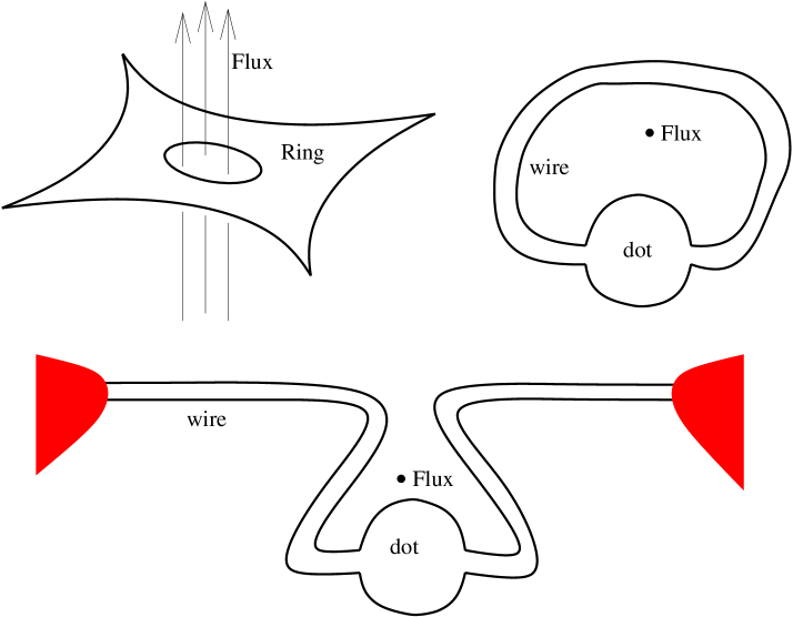
Figure 1: (a) Upper left: A chaotic ring that has the shape of a Sinai billiard, with Aharonov-Bohm flux. (b) Upper right: The dot-wire geometry with the same topology as in the case of the Sinai billiard. (c) Lower: The wire is cut into two leads that are attached to reservoirs. The latter is what we call “open geometry”.

The analysis of “quantum pumping” in closed systems should take into account several issues that go beyond the water analogy: (i) Kirchhoff law is not satisfied in the mesoscopic reality because charge can accumulate; (ii) There are quantized energy levels, consequently one has to distinguish between adiabatic and non-adiabatic dynamics; (iii) Interference is important, implying that the result of the calculation is of statistical nature (universal conductance fluctuations). On top we may have to take into account the effect of having an external environment (decoherence).

Quantum pumping is a special issue in the study of “driven systems”. We are going to emphasize the significance of “quantum chaos” in the analysis. This in fact provides the foundations for linear response theory (LRT) [1, 2, 3, 4, 5, 6]. We shall explain how to apply the Kubo formalism in order to analyze the dynamics in the low frequency (DC) regime. Within the Kubo formalism the problem boils down to the calculation of the generalized (DC) conductance matrix.

To avoid miss-understanding we emphasize that the dynamics in the low frequency (DC) regime is in general non-adiabatic: The DC conductance has both a dissipative and a non-dissipative parts. In the adiabatic limit (extremely small rate of driving) the dissipative part vanishes, while the non-dissipative part reduces to “adiabatic transport” (also called “geometric magnetism”) [7, 8, 9, 10]. The “adiabatic regime”, where the dissipative effect can be ignored, is in fact a tiny sub-domain of the relatively vast “DC regime”.

The dot-wire geometry of Fig.1b is of particular interest. We are going to discuss the special limit of taking the length of the wire ($L$) to be infinite. In this limit the adiabatic regime vanishes, but still we are left with a vast ”DC regime” where the pumping is described by a ”DC conductance”. In this limit we get results [11] that are in agreement with the well known analysis of quantum pumping [12, 13] in an open geometry (Fig.1c).

Figure 2: Detailed illustration of the dot-wire system. The dot potential is controlled by gate voltages $X_{1}$ and $X_{2}$. The flux through the loop is $X_{3}{=}\Phi$. The scattering region ($r{<}0$) is represented by an $S$ matrix. Later we assume that the length ($L$) of the wire is very large.

2 Driven systems

Consider a Fermi sea of non interacting “spinless” electrons. The electrons are bounded by some potential. To be specific we assume a ring topology as in Fig.1a. Of particular interest is the dot-wire geometry of Fig.1b, or its more elaborated version Fig.2. It has the same topology but we can distinguish between a “wire region” and a “dot region” (or “scattering region”). In particular we can consider a dot-wire system such that the length of the wire is very very long. If we cut the wire in the middle, and attach each lead to a reservoir, then we get the open geometry of Fig.1c.

We assume that we have some control over the potential that holds the electrons. Specifically, and without loss of generality, we assume that there are control parameters $X_{1}$ and $X_{2}$ that represent e.g. some gate voltages (see Fig.2) with which we can control the potential in the scattering region. Namely, with these parameters we can change the dot potential floor, or the height of some barrier, or the location of a “wall” element, or the position of a scatterer inside the dot. We call $X_{1}$ and $X_{2}$ shape parameters.

We also assume that it is possible to have an Aharonov-Bohm flux $X_{3}$ through the ring. Thus our notations are:

$$X_{1},X_{2}\ =\ \mbox{shape parameters}$$ (1)

$$X_{3}\ =\ \Phi\ =\ (\hbar/e)\phi\ =\ \mbox{magnetic flux}$$ (2)

and the motion of each electron is described by a one particle Hamiltonian

$$\mathcal{H}\ =\ \mathcal{H}(\bm{r},\bm{p};\ X_{1}(t),X_{2}(t),X_{3}(t))$$ (3)

To drive a system means to change some parameters (fields) in time. No driving means that $X_{1}$ and $X_{2}$ are kept constant, and also let us assume for simplicity that there is no magnetic field and that $X_{3}=0$. In the absence of driving we assume that the motion of the electrons inside the system is classically chaotic. For example this is the case with the so-called Sinai billiard of Fig.1a. In such circumstances the energy of the system is a constant of the motion, and the net circulating current is zero due to ergodicity.

The simplest way to create a current $\mathcal{I}$ in an open system (Fig.1c) is to impose bias by having a different chemical potential in each reservoir. Another possibility is to create an electro-motive-force (EMF) in the dot region. In linear response theory it can be proved that it does not matter what is the assumed distribution of the voltage along the “resistor”. The EMF is by Faraday law $-\dot{\Phi}$. Assuming DC driving (constant EMF), and the applicability of LRT, we get the “Ohm law” $\mathcal{I}=\bm{G}^{33}\times(-\dot{\Phi})$ and hence the transported charge is $dQ=-\bm{G}^{33}\ dX_{3}$. We call $\bm{G}^{33}$ the Ohmic (DC) conductance. If we have a low frequency AC driving rather than a DC driving, still the impedance (AC conductance) is expected to be well approximated by the DC conductance within a frequency range that we call the DC regime.

Yet another possibility is to induce current by changing shape parameter in time, while keeping either the bias or $X_{3}$ equal to zero. Say that we change $X_{1}$, then in complete analogy with Ohm law we can write $dQ=-\bm{G}^{31}\ dX_{1}$. More generally we can write

$$dQ\ =\ -\sum_{j}\bm{G}^{3j}\ dX_{j}$$ (4)

Obviously this type of formula makes sense only in the “DC regime” where the current at each moment of time depends only on the rates $\dot{X}_{j}$.

Figure 3: (a) Left: A driving cycle in $X$ space. In order to have non-zero area enclosed we have to change (without loss of generality) two parameters. (b) Right: In particular we consider pumping cycle in the $X_{3}=0$ plane (no magnetic field).

3 pumping cycles

In practice the interest is a time periodic (AC) driving. This means that the driving cycle can be represented by a closed contour at the $(X_{1},X_{2},X_{3})$ space as in Fig.3a. In fact we assume that the contour is lying in the $(X_{1},X_{2})$ plan as in Fig.3b. We ask what is the amount of charge which is transported via a section of the ring per cycle. Assuming the applicability of LRT we get in the DC regime

$$Q\ =\ \oint\mathcal{I}dt\ =\ \oint\bm{G}\cdot dX$$ (5)

where $X=(X_{1},X_{2},X_{3})$ and $\bm{G}=(\bm{G}^{31},\bm{G}^{32},\bm{G}^{33})$. Later we shall define a more general object $\bm{G}^{kj}$ with $k,j=1,2,3$ that we call generalized conductance matrix. In the above formula only the $k=3$ row enters into the calculation.

Getting $Q\neq 0$ means that the current has a non-zero DC component. So we can define “pumping” as getting DC current form AC driving. From the above it is clear that within the DC regime we have to vary at least two parameters to achieve a non-zero result. In a closed (in contrast to open) system this conclusion remains valid also outside of the DC regime, due to time reversal symmetry. In order to get DC current from one parameter AC driving, in a closed system, it is essential to have a non-linear response. Ratchets are non-linear devices that use “mixed” [15] or “damped” [14] dynamics in order to pump with only one parameter. We are not discussing such devices below.

4 What is the problem?

Most of the studies of quantum pumping were (so far) about open systems. Inspired by Landauer who pointed out that $\bm{G}^{33}$ is essentially the transmission of the device, Büttiker, Pretre and Thomas (BPT) have developed a formula that allows the calculation of $\bm{G}^{3j}$ using the $S$ matrix of the scattering region [12, 13]. It turns out that the non-trivial extension of this approach to closed systems involves quite restrictive assumptions [16]. Thus the case of pumping in closed systems has been left un-explored, except to some past works on adiabatic transport [9, 10]. Yet another approach to quantum pumping is to use the powerful Kubo formalism [6, 11, 17].

The Kubo formula, which we discuss later, gives a way to calculate the generalized conductance matrix $\bm{G}^{kj}$. It is a well know formula [1], so one can ask: what is the issue here? The answer is that both the validity conditions, and also the way to use the Kubo formula, are in fact open problems in physics.

The Van Kampen controversy regarding the validity of the Kubo formula in the classical framework is well known, and by now has been resolved. For a systematic classical derivation of the Kubo formula with all the validity conditions see Ref.[5] and references therein. The assumption of chaos is essential in the classical derivation. If this assumption is not satisfied (as in the trivial case of a driven 1D ring) then the Kubo formula becomes non-applicable.

What about the Quantum Mechanical derivation? The problem has been raised in Ref.[3] but has been answered only later in Refs.[4, 5] and follow up works. It is important to realize that the quantum mechanical derivation of the Kubo formula requires perturbation theory to infinite order, not just 1st order perturbation theory. We shall discuss later the non-trivial self consistency condition of the quantum mechanical derivation.

We note that the standard textbook derivation of the Kubo formula assumes that the energy spectrum is essentially a continuum. A common practice is to assume some weak coupling to some external bath [18]. However, this procedure avoids the question at stake, and in fact fails to take into consideration important ingredients that have to do with quantum chaos physics. In this lecture the primary interest is in the physics of a closed isolated system. Only in a later stage we look for the effects that are associated with having a weak coupling to an external bath.

Why do we say that it is not clear how to use the Kubo formula? We are going to explain that the quantum mechanical derivation of the Kubo formula introduces an energy scale that we call $\Gamma$. It plays an analogous role to the level broadening parameter which is introduced in case of a coupling to a bath. Our $\Gamma$ depends on the rate $\dot{X}$ of the driving in a non-trivial way. One may say that $\Gamma$ in case of an isolated system is due to the non-adiabaticity of the driving. Our $\Gamma$ affects both the dissipative and the non-dissipative (geometric) part of the response. Without a theory for $\Gamma$ the quantum mechanical Kubo formula is ill defined.

5 Generalized forces and currents

Given a Hamiltonian we define generalized forces in the conventional way:

$$\mathcal{F}^{k}\ =\ -\frac{\partial\mathcal{H}}{\partial X_{k}}$$ (6)

one obvious reasoning that motivates this definition follows from writing the following (exact) expression for the change in the energy $E=\langle\mathcal{H}\rangle$ of the system:

$$E_{\mbox{\tiny final}}-E_{\mbox{\tiny initial}}\ =\ -\int\langle\mathcal{F}(t)\rangle\cdot dX$$ (7)

In particular we note that $\mathcal{F}^{3}$ should be identified as the current $\mathcal{I}$. This identification can be explained as follows: If we make a change $d\Phi$ of the flux during a time $dt$, then the EMF is $-d\Phi/dt$, leading to a current $\mathcal{I}$. The energy increase is the EMF times the charge, namely $dE=(-d\Phi/dt)\times(\mathcal{I}dt)=-\mathcal{I}d\Phi$. Hence $\mathcal{I}$ is conjugate to $\Phi$.

As an example we consider [17] a network model [19]. See the illustration of Fig.4d. The Hamiltonian is

$$\mathcal{H}\ \ =\ \ \mbox{\small network}\ \ +\ \ X_{2}\ \delta(x-X_{1})$$ (8)

We assume control over the position $X_{1}$ of the delta scatterer, and also over the “height” $X_{2}$ of the scatterer. By the definition we get:

$$\mathcal{F}^{1}\ = \ X_{2}\delta^{\prime}(x-X_{1})$$ (9)

$$\mathcal{F}^{2}\ = \ -\delta(x-X_{1})$$ (10)

Note that $\mathcal{F}^{1}$ is the ordinary Newtonian force which is associated with translations. Its operation on the wavefunction can be realized by the differential operator

$$\mathcal{F}^{1}\ \ \mapsto\ \ -X_{2}\left(\overrightarrow{\partial}+\overleftarrow{\partial}-\frac{2\mathsf{m}}{\hbar^{2}}X_{2}\right)_{x=X_{1}+0}$$ (11)

where we have used the matching condition across the delta function and $\mathsf{m}$ is the mass of the particle.

What about the current operator? For its definition we have to introduce a vector potential $\mathcal{A}(x)=\Phi a(x)$ into the Hamiltonian such that

$$\oint\overrightarrow{\mathcal{A}}\cdot\overrightarrow{dr}\ =\ \Phi$$ (12)

Thus we have to specify $a(x)$, which describes how the vector potential varies along the loop. This is not merely a gauge freedom because the electric field $-\dot{\Phi}a(x)$ is a measurable quantity. Moreover, a different $a(x)$ implies a different current operator. In particular we can choose $a(x)$ to be a delta function across a section $x=x_{0}$. Then we get:

$$\mathcal{I}\ \ =\ \ \frac{e}{2\mathsf{m}}\left(\delta(x-x_{0})p+p\delta(x-x_{0})\right)$$ (13)

Note that the operation of this operator can be realized by the differential operator

$$\mathcal{I}\ \ \mapsto\ \ -i\frac{e\hbar}{2\mathsf{m}}\Big{(}\overrightarrow{\partial}-\overleftarrow{\partial}\Big{)}_{x=x_{0}}$$ (14)

A few words are in order regarding the continuity of the charge flow. It should be clear that in any moment the current through different sections of a wire does not have to be the same, because charge can accumulate. Kirchhoff law is not satisfied. For example if we block the left entrance to the dot in Fig.2, and raise the dot potential, then current is pushed out of the right lead, while the current in the blocked side is zero. Still if we make a full pumping cycle, such that the charge comes back to its original distribution at the end of each cycle, then the result for $Q$ should be independent of the section through which the current is measured.

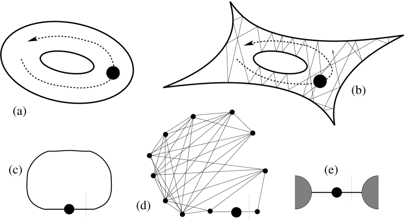
Figure 4: A scatterer (represented by a black circle) is translated through a system that has a Fermi occupation of spinless non-interacting electrons. In (a) the system is a simple ring. In (b) it is a chaotic ring (Sinai billiard). In (c) and in (d) we have network systems that are of the same type of (a) and (b) respectively. In the network, the scatterer (“piston”) is a delta function (represented as a big circle) located at $x=X_{1}$. The current is measured through $x=x_{0}$ (dotted vertical line). In (e) we have an open geometry with left and right leads that are attached to reservoirs that have the same chemical potential.

6 Linear response theory

Assume that $X(t)=X^{(0)}+\delta X(t)$, and look for a quasi-stationary solution. To have linear response means that the generalized forces are related to the driving as follows:

$$\langle\mathcal{F}(t)\rangle\ =\ \langle\mathcal{F}\rangle_{0}\ +\ \int_{-\infty}^{\infty}\bm{\alpha}(t-t^{\prime})\cdot\delta X(t^{\prime})\ dt^{\prime}$$ (15)

where $\langle...\rangle_{0}$ denote the expectation value with respect to the unperturbed $X(t)=X^{(0)}$ stationary state. From now on we disregard the zero order term (the “conservative force”), and focus on the linear term. The generalized susceptibility $\chi^{kj}(\omega)$ is the Fourier transform of the (causal) response kernel $\alpha^{kj}(\tau)$, while the generalized conductance matrix is defined as

$$\bm{G}^{kj}\ =\ \left.\frac{\mbox{Im}[\chi^{kj}(\omega)]}{\omega}\ \right|_{\omega\sim 0}\ =\ \bm{\eta}^{kj}+\bm{B}^{kj}$$ (16)

The last equality defines the symmetric and the anti-symmetric matrices $\bm{\eta}^{kj}$ and $\bm{B}^{kj}$. Thus in the DC limit Eq.(15) reduces to a generalized Ohm law:

$$\langle\mathcal{F}^{k}\rangle\ \ =\ \ -\sum_{j}\bm{G}^{kj}\ \dot{X}_{j}$$ (17)

which can be written in fancy notations as

$$\langle F\rangle\ \ =\ \ -\bm{G}\cdot\dot{X}\ \ =\ \ -\bm{\eta}\cdot\dot{X}\ -\ \bm{B}\wedge\dot{X}$$ (18)

Note that the rate of dissipation is

$$\dot{\mathcal{W}}\ \ =\ \ -\langle F\rangle\cdot\dot{X}\ \ =\ \ \sum_{kj}\bm{\eta}^{kj}\ \dot{X}_{k}\ \dot{X}_{j}$$ (19)

We would like to focus not on the dissipation issue, but rather on the transport issue. From Eq.(5) we get

$$Q\ \ =\ \ \Big{[}\ -\oint\bm{\eta}\cdot dX\ \ -\oint\bm{B}\wedge dX\ \ \Big{]}_{k=3}$$ (20)

From now on we consider a planar $(X_{1},X_{2})$ pumping cycle, and assume that there is no magnetic field. Then it follows from time reversal symmetry [Onsager] that $\bm{\eta}^{31}=\bm{\eta}^{32}=0$, and consequently

$$Q\ =\ -\oint\overrightarrow{\bm{B}}\cdot\ \overrightarrow{ds}$$ (21)

where $\overrightarrow{\bm{B}}=(\bm{B}^{23},\bm{B}^{31},\bm{B}^{12})$, with $\bm{B}^{12}=0$, and $\overrightarrow{ds}=(dX_{2},-dX_{1},0)$ is a normal vector in the pumping plane as in Fig.3b.

The various objects that have been defined in this section are summarized by the following diagram:

7 The Kubo formula

The Kubo formula for the response kernel is

$$\alpha^{kj}(\tau)\ =\ \Theta(\tau)\times\frac{i}{\hbar}\langle[\mathcal{F}^{k}(\tau),\mathcal{F}^{j}(0)]\rangle_{0}$$ (22)

where the expression on the right hand side assumes a zero order $X=X^{0}$ stationary state (the so called “interaction picture”), and $\Theta(\tau)$ is the step function.

Using the definitions of the previous section, and assuming a Fermi sea of non-interacting fermions with occupation function $f(E)$, we get the following expressions:

$$\bm{\eta}^{kj} = -\pi\hbar\sum_{n,m}\frac{f(E_{n}){-}f(E_{m})}{E_{n}{-}E_{m}}\mathcal{F}^{k}_{nm}\mathcal{F}^{j}_{mn}\ \delta_{\Gamma}(E_{m}{-}E_{n})$$

$$\bm{B}^{kj} = 2\hbar\sum_{n}f(E_{n})\sum_{m(\neq n)}\frac{\mbox{Im}\left[\mathcal{F}^{k}_{nm}\mathcal{F}^{j}_{mn}\right]}{(E_{m}{-}E_{n})^{2}+(\Gamma/2)^{2}}$$ (23)

We have incorporated in these expression a broadening parameter $\Gamma$ which is absent in the “literal” Kubo formula. If we set $\Gamma=0$ we get no dissipation ($\bm{\eta}=0$). We also see that $\Gamma$ affects the non-dissipative part of the response. Thus we see that without having a theory for $\Gamma$ the Kubo formula is an ill defined expression.

8 Adiabatic transport (Geometric magnetism)

The “literal” Kubo formula (i.e. with $\Gamma=0$) has been considered in Refs.([9, 10]). In this limit we have no dissipation ($\bm{\eta}=0$). But we may still have a non-vanishing $\bm{B}$. By Eq.(23) the total $\bm{B}$ is a sum over the occupied levels. The contribution of a given occupied level $n$ is:

$$\bm{B}^{kj}_{n}\ \ =\ \ 2\hbar\sum_{m(\neq n)}\frac{\mbox{Im}\left[\mathcal{F}^{k}_{nm}\mathcal{F}^{j}_{mn}\right]}{(E_{m}-E_{n})^{2}+(\Gamma/2)^{2}}$$ (24)

with $\Gamma=0$. This is identified as the geometric magnetism of Ref.[10].

We can get some intuition for $\overrightarrow{\bm{B}}$ from the theory of adiabatic processes. The Berry phase is given as a line integral $(1/\hbar)\oint\overrightarrow{\bm{A}}\cdot dX$ over “vector potential” in $X$ space. By stokes law it can be converted to an integral $(1/\hbar)\int\!\!\!\!\int\overrightarrow{\bm{B}}\cdot dS$ over a surface that is bounded by the driving cycle. The $\overrightarrow{\bm{B}}$ field is divergence-less, but it may have singularities at $X$ points where the level $n$ has a degeneracy with a nearby level. We can regard these points as the location of magnetic charges. The result of the surface integral should be independent of the choice of the surface modulo $2\pi$, else Berry phase would be ill defined. Therefore the net flux via a closed surface (which we can regard as formed of two Stokes surfaces) should be zero modulo $2\pi$. Thus, if we have a charge within a closed surface it follows by Gauss law that it should be quantized in units of $(\hbar/2)$. These are the so called “Dirac monopoles”. In our setting $X_{3}$ is the Aharonov-Bohm flux. Therefore we have vertical “Dirac chains”

$$\mbox{chain}\ =\ \left(X_{1}^{(0)},\ \ X_{2}^{(0)},\ \ \Phi^{(0)}+2\pi\frac{e}{\hbar}\times\mbox{\small integer}\right)$$ (25)

In the absence of any other magnetic field we have time-reversal symmetry for either integer or half integer flux. It follows that there are two types of Dirac chains: those that have a monopole in the plane of the pumping cycle, and those that have their monopoles half unit away from the pumping plane.

In the next section we shall see how these observations help to analyze the pumping process. We shall also illuminate the effect of having $\Gamma\neq 0$. Later we shall discuss the “physics” behind $\Gamma$.

9 Quantized pumping?

The issue of quantized pumping is best illustrated by the popular two delta barrier model, which is illustrated in Fig.5. The “dot region” $|Q|<a/2$ is described by the potential

$$U(r;X_{1},X_{2})=X_{1}\delta\left(x+\frac{a}{2}\right)+X_{2}\delta\left(x-\frac{a}{2}\right)$$ (26)

The pumping cycle is described in Fig.5c. In the 1st half of the cycle an electron is taken from the wire into the dot region via the left barrier, while in the second half of the cycle an electron is transfered from the dot region to the wire via the right barrier. So it seems that one electron is pumped through the device per cycle. The question is whether it is exactly one electron ($Q=e$) or not?

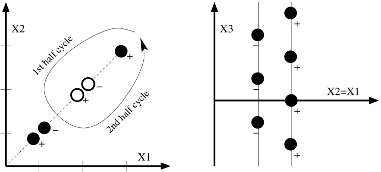
Figure 5: (a) Upper left: The energy levels of a ring with two barriers, at the beginning of the pumping cycle. It is assumed that the three lower levels are occupied. (b) Upper right: The adiabatic levels as a function of time during the pumping cycle. (c) Lower Left: The $(X_{1},X_{2})$ locations of the Dirac chains of the $3$ occupied levels. Filled (hollow) circles imply that there is (no) monopole in the pumping plane. Note that for sake of illustration overlapping chains are displaced from each other. The pumping cycle encircles $2+1$ Dirac chains that are associated with the 3rd and 2nd levels respectively. (d) Lower right: The $2$ Dirac chains that are associated with the 3rd level.

In the case of an open geometry the answer is known [20, 21]. Let us denote by $g_{0}$ the average transmission of the dot region for $X$ values along the pumping cycle. In the limit $g_{0}\rightarrow 0$, which is a pump with no leakage, indeed one gets $Q=e$. Otherwise one gets $Q=(1-g)e$.

What about a closed (ring) geometry? Do we have a similar result? It has been argued [20] that if the the pumping process is strictly adiabatic then we get exactly $Q=e$. We are going to explain below that this is in fact not correct: We can get either $Q<1$ or $Q>1$ or even $Q\gg 1$.

Recall that by Eq.(21) the pumped charge $Q$ equals the projected flux of the $\overrightarrow{\bm{B}}$ field through the pumping cycle (Fig.3b). If the charge of the monopoles were uniformly distributed along the chains, it would follow that $Q$ is exactly quantized. But this is not the case, and therefore $Q$ can be either smaller or larger than $1$ depending on the type of chain(s) being encircled. In particular, in case of a tight cycle around a monopole we get $Q\gg e$ which is somewhat counter-intuitive, while if the monopole is off-plane $Q<e$.

What is the effect of $\Gamma$ on this result? It is quite clear that $\Gamma$ diminishes the contribution of the singular term. Consequently it makes $Q$ less than one. This gives us a hint that the introduction of $\Gamma$ might lead to a result which is in agreement with that obtained for an open geometry. We shall discuss this issue in the next sections.

10 The Kubo Formula and “quantum chaos”

We turn now to discuss $\Gamma$. Any generic quantum chaos system is characterized by some short correlation time $\tau_{cl}$, by some mean level spacing $\Delta$, and by a semiclassical energy scale that we denote as $\Delta_{b}$. Namely:

$$\Delta\ \propto \ \hbar^{d}/\mbox{\small volume}\ =\ \mbox{\small mean level spacing}$$ (27)

$$\Delta_{b}\ \sim \ \hbar/\tau_{\mbox{\tiny cl}}\ =\ \mbox{\small bandwidth}$$ (28)

The term bandwidth requires clarification. If we change a parameter $X$ in the Hamiltonian $\mathcal{H}$, then the perturbation matrix $\mathcal{F}_{nm}$ has non-vanishing matrix elements within a band $|E_{n}-E_{m}|<\Delta_{b}$. These matrix elements are characterized by some root-mean-square magnitude $\sigma$, while outside of the band the matrix elements are very small.

If the system is driven slowly in a rate $\dot{X}$ then levels are mixed non-perturbatively. Using a quite subtle reasoning [4, 5, 6, 2] the relevant energy range for the non-perturbative mixing of levels is found to be

$$\Gamma\ \ =\ \ \left(\frac{\hbar\sigma}{\Delta^{2}}|\dot{X}|\right)^{2/3}\!\times\Delta\ \ \ \ \propto\ \ \ \ \left(L\frac{}{}|\dot{X}|\right)^{2/3}\frac{1}{L}$$ (29)

The latter equality assumes dot-wire geometry as in Fig.1b, where $L$ is the length of the wire. Now we can distinguish between three $\dot{X}$ regimes:

$$\Gamma\ll\Delta$$ adiabatic regime (30)

$$\Delta<\Gamma<\Delta_{b}$$ non-adiabatic regime (31)

otherwise non-perturbative regime (32)

In the adiabatic regime levels are not mixed by the driving, which means that the system (so to say) follows the same level all the time. In the perturbative regime there is a non-perturbative mixing on small energy scales, but on the large scale we have Fermi-Golden-Rule (FGR) transitions. If the self consistency condition ($\Gamma\ll\Delta_{b}$) breaks down, then the FGR picture becomes non-applicable, and consequently $\Gamma$ becomes a meaningless parameter.

In the non-perturbative regime we expect semiclassical methods to be effective, provided the system has a classical limit (which is not the case with random matrix models [22]). In general one can argue that in the limit of infinite volume (or small $\hbar$) perturbation theory always breaks down, leading to a semiclassical behavior. But in the dot-wire geometry this is not the case if we take the limit $L\rightarrow\infty$, keeping the width of the wire fixed. With such limiting procedure Eq.(29) implies that the self-consistency condition $\Gamma\ll\Delta_{b}$ is better and better satisfied! This means that the Kubo formula can be trusted. Furthermore, with the same limiting procedure the $L\rightarrow\infty$ is a non-adiabatic limit because the adiabaticity condition $\Gamma\ll\Delta$ breaks down.

11 Kubo formula using an FD relation

The Fluctuation-dissipation (FD) relation allows us to calculate the conductance $\bm{G}^{kj}$ from the correlation function $C^{kj}(\tau)$ of the generalized forces. In what follows we use the notations:

$$K^{kj}(\tau)\ = \ \frac{i}{\hbar}\langle[\mathcal{F}^{k}(\tau),\mathcal{F}^{j}(0)]\rangle_{0}$$ (33)

$$C^{kj}(\tau)\ = \ \frac{1}{2}\left(\langle\mathcal{F}^{k}(\tau)\mathcal{F}^{j}(0)\rangle_{0}+cc\right)$$ (34)

Their Fourier transforms are denoted $\tilde{K}^{kj}(\omega)$ and $\tilde{C}^{kj}(\omega)$. The expectation value above assumes a zero order stationary preparation. We shall use subscript $|_{F}$ to indicate many-body Fermi occupation. We shall use the subscript $|_{T}$ or the subscript $|_{E}$ to denote one-particle canonical or microcanonical preparation. At high temperatures the Boltzmann approximation applies and we can use the exact relation $f(E_{n}){-}f(E_{m})=\tanh((E_{n}{-}E_{m})/(2T))\times(f(E_{n}){+}f(E_{m}))$ so as to get

$$\tilde{K}^{kj}_{F}(\omega)=i\omega\times\frac{2}{\hbar\omega}\tanh\left(\frac{\hbar\omega}{2T}\right)\ C^{kj}_{T}(\omega)$$ (35)

At low temperatures we can use the approximation $f(E){-}f(E^{\prime})\approx-\frac{1}{2}[\delta_{T}(E{-}E_{F})+\delta_{T}(E^{\prime}{-}E_{F})]\times(E{-}E^{\prime})$ with $\delta_{T}(E{-}E_{F})=-f^{\prime}(E)$ so as to get

$$\tilde{K}^{kj}_{F}(\omega) \approx i\omega\times g(E)\ \tilde{C}^{kj}_{E_{F}}(\omega)$$ (36)

The application of this approximation is “legal” if we assume temperature $T\gg\Delta_{b}$. This is a very “bad” condition because for (e.g.) ballistic dot $\Delta_{b}$ is the relatively large Thouless energy. However, we can regard the large $T$ result as an $E_{F}$ averaged zero temperature calculation. Then it can be argued that for a quantum chaos system with a generic bandprofile the average is in fact the “representative” result (see discussion of “universal conductance fluctuation” in later sections).

Substituting the Kubo formula $\alpha^{kj}(\tau)=\Theta(\tau)\ K^{kj}(\tau)$ in the definition of $\bm{G}^{kj}$, and using the latter relation between $K^{kj}(\tau)$ and $C^{kj}(\tau)$ we get after some straightforward algebra the following expression for the conductance:

$$\bm{G}^{kj}=\int_{0}^{\infty}K_{F}^{kj}(\tau)\tau d\tau\ \approx\ \mathsf{g}(E_{F})\int_{0}^{\infty}C_{E_{F}}^{kj}(\tau)d\tau$$ (37)

where $\mathsf{g}(E_{F})$ is the density of the one-particle states. If we want to incorporate $\Gamma$ the recipe is simply:

$$C(\tau)\ \ \mapsto\ \ C(\tau)\ \mbox{e}^{-\frac{1}{2}(\Gamma/\hbar)|\tau|}$$ (38)

The expression of $\bm{G}^{kj}$ using $C^{kj}(\tau)$ is a generalized FD relation. It reduces to the standard FD relation if we consider the dissipative part:

$$\bm{\eta}^{kj}\ =\ \frac{1}{2}\mathsf{g}(E_{F})\tilde{C}_{E_{F}}^{kj}(\omega\sim 0)$$ (39)

whereas the non-dissipative part requires integration over all the frequencies (see next section).

12 Kubo via Green functions or $S$ matrix

Now we would like to express $\bm{G}^{kj}$ using Green functions, and eventually we would like to express it using the $S$ matrix of the scattering region. The first step is to rewrite the FD relation as follows:

$$\bm{G}^{kj}\ \ = \ \ \hbar\mathsf{g}(E_{F})\int_{-\infty}^{\infty}\frac{-i\tilde{C}_{E_{F}}^{kj}(\omega)}{\hbar\omega-i(\Gamma/2)}\ \frac{d\omega}{2\pi}$$ (40)

The second step is to write

$$C^{kj}_{E}(\omega)=\frac{\hbar}{2\mathsf{g}(E)}\left[C^{kj}(E{+}\hbar\omega,E)+C^{jk}(E{-}\hbar\omega,E)\right]$$ (41)

where

$$C^{kj}(E^{\prime},E) = 2\pi\sum_{nm}\mathcal{F}^{k}_{nm}\delta(E^{\prime}-E_{m})\mathcal{F}^{j}_{mn}\delta(E-E_{n})$$ (42)

$$= \frac{2}{\pi}\ \mbox{trace}\left[\mathcal{F}^{k}\ \mbox{Im}[\mathsf{G}(E^{\prime})]\ \mathcal{F}^{j}\ \mbox{Im}[\mathsf{G}(E)]\right]$$ (43)

We use the standard notations $\mathsf{G}(z)=1/(z-\mathcal{H})$, and $\mathsf{G}^{\pm}(E)=G(E{\pm}i0)$, and $\mbox{Im}[\mathsf{G}]=-i(\mathsf{G}^{+}{-}\mathsf{G}^{-})/2=-\pi\delta(E{-}\mathcal{H})$. After some straightforward algebra we get:

$$\bm{G}^{kj}=i\frac{\hbar}{2\pi}\mbox{trace}\left[\mathcal{F}^{k}\mathsf{G}(E_{F}{-}i\Gamma/2)\mathcal{F}^{j}\mbox{Im}[\mathsf{G}(E_{F})]\right.$$

$$-\left.\mathcal{F}^{k}\mbox{Im}[\mathsf{G}(E_{F})]\mathcal{F}^{j}\mathsf{G}(E_{F}{+}i\Gamma/2)\right]$$ (44)

For the dot-wire geometry in the limit $L\rightarrow\infty$ we can treat the $i\Gamma$ as if it were the infinitesimal $i0$. Some more non-trivial steps allow us to reduce the trace operation to the boundary ($r=0$) of the scattering region (Fig.2), and then to express the result using the $S$ matrix. Disregarding insignificant interference term that has to do with having “standing wave” the result is:

$$\bm{G}^{3j}\ =\ \frac{e}{2\pi i}\mbox{trace}\left(P_{\mbox{\tiny A}}\frac{\partial S}{\partial X_{j}}S^{{\dagger}}\right)$$ (45)

This formula, which we derive here using “quantum chaos” assumptions is the same as the BPT formula that has been derived for an open geometry. It is important to remember that the limit $L\rightarrow\infty$ is a non-adiabatic limit ($\Gamma\gg\Delta$). Still it is a “DC limit”. Therefore what we get here is “DC conductance” rather than “adiabatic pumping”. The latter term is unfortunately widely used in the existing literature.

13 The prototype pumping problem

What is the current which is created by translating a scatterer (“piston”)? This is a “pumping” question. Various versions of the assumed geometry are illustrated in Fig.4. Though it sounds simple this questions contains (without loss of generality) all the ingredients of a typical pumping problem. Below we address this question first within a classical framework, and then within quantum mechanics.

The simplest case is to translate a scatterer in 1D ring (Fig.4a). Assuming that there is no other scattering mechanism it is obvious that the steady state solution of the problem is:

$$dQ=1\times\frac{e}{\pi}k_{\mbox{\tiny F}}\times dX$$ (46)

We assume here Fermi occupation, but otherwise this result is completely classical. This result holds for any nonzero ”size” of scatterer, though it is clear that in the case of a tiny scatterer it would take a much longer time to attain the steady state. Also note that there is no dissipation in this problem. The steady state solution is an exact solution of the problem.

The picture completely changes if we translate a scatterer inside a chaotic ring (Fig.4b). In such case the problem does not possess a steady state solution. Still there is a quasi steady state solution. This means that at any moment the state is quasi-ergodic: If we follow the evolution for some time we see that there is slow diffusion to other energy surfaces (we use here phase space language). This diffusion leads to dissipation as explained in [5] (and more Refs therein). However, we are interested here mainly in the transport issue. As the scatterer pushes its way through the ergodizing distribution, it creates a current. Obviously the size of the scatterer do matter in this case. Using classical stochastic picture we can derive the following result:

$$dQ=\left[\frac{g_{T}}{1{-}g_{T}}\right]\left[\frac{1{-}g_{0}}{g_{0}}\right]\times\frac{e}{\pi}k_{\mbox{\tiny F}}\times dX$$ (47)

where $g_{0}$ is the transmission or the relative size of the moving scatterer, while $g_{T}$ is the overall transmission of the ring.

What about the quantum mechanical analysis? We shall show that the same result is obtained on the average. This means that the classical expression still holds, but only in a statistical sense. This is in close analogy with the idea of “universal conductance fluctuations”. We shall discuss the effect of $\Gamma$ on the distribution of $\bm{G}$.

It should be noticed that our quantum chaos network model (Fig.4d) essentially generalizes the two barrier model. Namely, one delta function is the “scatterer” and the other delta functions is replaced by a complicated “black box”. Let us use the term “leads” in order to refer to the two bonds that connect the “black box” to the scatterer. Now we can ask what happens (given $\dot{X_{1}}$) if we take the length of the leads to be very very long. As discussed previously this is a non-adiabatic limit. We shall explain that in this limit we expect to get the same result as in the case of an open geometry. For the latter the expected result is [23]:

$$dQ=(1{-}g_{0})\times\frac{e}{\pi}k_{\mbox{\tiny F}}\times dX$$ (48)

We shall explain how Eq.(47) reduces to Eq.(48). The latter is analogous to the Landauer formula $\bm{G}^{33}=(e^{2}/2\pi\hbar)g_{0}$. The charge transport mechanism which is represented by Eq.(48) has a very simple heuristic explanation, which is reflected in the term “snow plow dynamics” [23].

Figure 6: The average conductance $\bm{G}^{31}$ for the network of Fig.4d. The average is taken over more than 20000 levels around $E_{F}$, while the calculation (for each Fermi level) was performed in an interval of 32000 levels. The transmission of the “piston” is $g_{0}\approx 0.1$. The perpendicular dotted line indicates the border of the regime where the Kubo calculation is valid. We also plot the standard deviation, while the inset displays the distribution for $\Gamma=0.0001\Delta$.

14 Analysis of the network model

One way to calculate $\bm{G}^{31}$ for the network model of Fig.4d is obviously to do it numerically using Eq.(23). For this purpose we find the eigenstates of the network, and in particular the wavefunctions $\psi^{n}=A_{n}\sin(k_{n}x+\varphi_{n})$ at (say) the right lead. Then we calculate the matrix elements

$$\mathcal{I}_{nm} = -i\frac{e\hbar}{2\mathsf{m}}\left(\psi^{n}\partial\psi^{m}-\partial\psi^{n}\psi^{m}\right)_{x{=}x_{0}}$$ (49)

$$\mathcal{F}_{nm} = -\lambda\frac{\hbar^{2}}{2\mathsf{m}}\left(\psi^{n}\partial\psi^{m}+\partial\psi^{n}\psi^{m}-\lambda\psi^{n}\psi^{m}\right)_{x=X_{1}+0}$$ (50)

and substitute into Eq.(23). The distribution that we get for $\bm{G}^{31}$, as well as the dependence of average and the variance on $\Gamma$ are presented in Fig.6. We see that $\Gamma$ reduces the fluctuations. If we are deep in the regime $\Delta\ll\Gamma\ll\Delta_{b}$ the variance becomes very small and consequently the average value becomes an actual estimate for $\bm{G}^{31}$. This average value coincides with the “classical” (stochastic) result Eq.(47) as expected on the basis of the derivation below.

In order to get an expression for $\bm{G}^{31}$ it is most convenient to use the FD expression Eq.(37). For this purpose we have to calculate the cross correlation function of $\mathcal{I}$ and $\mathcal{F}^{1}$ which we denote simply as $C(\tau)$. If we describe the dynamics using a stochastic picture [17] we get that $C(\tau)$ is a sum of delta spikes:

$$C(\tau)\ =\ e\frac{v_{\mbox{\tiny F}}}{2L}2\mathsf{m}v_{\mbox{\tiny F}}\left[(1-g_{0})\sum_{\pm}\pm\delta(\tau\pm\tau_{1})\right]+{....}$$ (51)

where $\tau_{1}=(x_{0}-X_{1})/v_{\mbox{\tiny F}}$ is the time to go from $X_{1}$ to $x_{1}$ with the Fermi velocity $v_{\mbox{\tiny F}}$, and the dots stand for more terms due to additional reflections. If we integrate only over the short correlation then we get

$$\int_{0}^{\mbox{short}}C(\tau)d\tau\ \ =\ \ -e\frac{\mathsf{m}v_{\mbox{\tiny F}}^{2}}{L}\left[1-g_{0}\right]$$ (52)

while if we include all the multiple reflections we get a geometric sum that leads to [17]:

$$\int_{0}^{\infty}C(\tau)d\tau\ \ =\ \ -e\frac{\mathsf{m}v_{\mbox{\tiny F}}^{2}}{L}\left[\frac{1-g_{0}}{g_{0}}\right]\left[\frac{g_{T}}{1-g_{T}}\right]$$ (53)

This leads to the result that was already mentioned in the previous section:

$$\bm{G}^{31}=-\left[\frac{1-g_{0}}{g_{0}}\right]\left[\frac{g_{T}}{1-g_{T}}\right]\times\frac{e}{\pi}k_{\mbox{\tiny F}}$$ (54)

We also observe that if the scattering in the outer region results in “loss of memory”, then by Eq.(38) only the short correlation survives, and we get

$$\bm{G}^{31}=-(1-g_{0})\times\frac{e}{\pi}k_{\mbox{\tiny F}}$$ (55)

Technically this is a special case of Eq.(54) with the substitution of the serial resistance $(1{-}g_{T})/g_{T}=(1{-}g_{0})/g_{0}+(1{-}0.5)/0.5$.

The stochastic result can be derived also using a proper quantum mechanical calculation [17]. The starting point is the following (exact) expression for the Green function:

$$\langle x|\mathsf{G}(E)|x_{0}\rangle\ \ =\ \ -\frac{i}{\hbar v_{F}}\sum_{p}A_{p}\mbox{e}^{ik_{E}L_{p}}$$ (56)

The sum is over all the possible trajectories that connect $x_{0}$ and $x$. More details on this expression the the subsequent calculation can be found in Ref.[17]. The final result for the average conductance coincides with the classical stochastic result.

15 Summary

Linear response theory is the major tool for study of driven systems. It allows to explore the crossover from the strictly adiabatic “geometric magnetism” regime to the non-adiabatic regime. Hence it provides a unified framework for the theory of pumping.

• “Quantum chaos” considerations in the derivation of the Kubo formula for the case of a closed isolated system are essential ($\Gamma\propto|\dot{X}|^{2/3}$).

• We have distinguished between adiabatic, non-adiabatic and non-perturbative regimes, depending on what is $\Gamma$ compared with $\Delta$ and $\Delta_{b}$.

• In the strict adiabatic limit Kubo formula reduces to the familiar adiabatic transport expression (“geometric magnetism”).

• A generalized Fluctuation-dissipation relation can be derived. In the zero temperature limit an implicit assumption in the derivation is having a generic bandprofile as implied by quantum chaos considerations.

• We also have derived an $S$ matrix expression for the generalized conductance of a dot-wire system, in the non-adiabatic limit $L\rightarrow\infty$. The result coincides with that of open system (BPT formula).

• The issue of “quantized pumping” is analyzed by regarding the field which is created by “Dirac chains”. In the adiabatic regime $Q$ can be either smaller or larger than unity, while in the non-adiabatic regime $Q$ is less than unity in agreement with BPT.

• We have analyzed pumping on networks using Green function expressions. The average result can be expressed in terms of transmission probabilities. The analog of universal conductance fluctuations is found in the strict adiabatic regime. The conductance becomes well define (small dispersion) in the non-adiabatic regime.

• The average over the quantum mechanical result, which becomes the well defined conductance in the non-adiabatic regime, coincides with the result that had been obtained for the corresponding stochastic model.

16 Acknowledgments

I have the pleasure to thank T. Kottos and H. Schanz for fruitful collaboration, and Y. Avishai, M. Büttiker, T. Dittrich, M. Moskalets and K. Yakubo for discussions. This research was supported by the Israel Science Foundation (grant No.11/02), and by a grant from the GIF, the German-Israeli Foundation for Scientific Research and Development.

http://www.bgu.ac.il/$\sim$dcohen/

References

- [1] L.D. Landau and E.M. Lifshitz, Statistical physics, (Buttrworth Heinemann 2000).
- [2] D. Cohen in Dynamics of Dissipation, Proceedings of the 38th Karpacz Winter School of Theoretical Physics, Edited by P. Garbaczewski and R. Olkiewicz (Springer, 2002)
- [3] M. Wilkinson, J. Phys. A 21 (1988) 4021. M. Wilkinson and E.J. Austin, J. Phys. A 28 (1995) 2277.
- [4] D. Cohen, Phys. Rev. Lett. 82 (1999) 4951.
- [5] D. Cohen, Annals of Physics 283 (2000) 175.
- [6] D. Cohen, Phys. Rev. B 68 (2003) 155303.
- [7] M.V. Berry, Proc. R. Soc. Lond. A 392 (1984) 45.
- [8] D. J. Thouless, Phys. Rev. B27 (1983) 6083.
- [9] J.E. Avron et al, Rev. Mod. Phys. 60 (1988) 873.
- [10] M.V. Berry and J.M. Robbins, Proc. R. Soc. Lond. A 442 (1993) 659.
- [11] D. Cohen, Phys. Rev. B 68 (2003) 201303(R).
- [12] M. Büttiker et al, Z. Phys. B-Condens. Mat., 94 (1994) 133.
- [13] P. W. Brouwer, Phys. Rev. B 58 (1998) R10135.
- [14] P.Reimann, Phys. Rep. 361 (2002) 57. Special issue, Appl. Phys. A 75 (2002). P.Reimann, M. Grifoni, and P.Hanggi, Phys. Rev. Lett. 79 (1997) 10.
- [15] H. Schanz, M.F. Otto, R. Ketzmerick, and T. Dittrich, Phys. Rev. Lett. 87 (2001) 070601.
- [16] M. Moskalets and M. Büttiker, Phys. Rev. B 68 (2003) 161311(R).
- [17] D. Cohen, T. Kottos and H. Schanz, Phys. Rev. E 71 (2005) 035202(R).
- [18] Y. Imry and N.S. Shiren, Phys. Rev. B 33 (1986) 7992.
- [19] T. Kottos and U. Smilansky. Phys. Rev. Lett. 79 (1997) 4794.
- [20] T. A. Shutenko, I. L. Aleiner and B. L. Altshuler, Phys. Rev. B61 (2000) 10366.
- [21] Y. Levinson, O. Entin-Wohlman, and P. Wolfle, cond-mat/0010494. M. Blaauboer and E.J. Heller, Phys. Rev. B 64 (2001) 241301(R).
- [22] D. Cohen and T. Kottos, Phys. Rev. Lett. 85 (2000) 4839.
- [23] J. E. Avron et al, Phys. Rev. B 62, R10 (2000) 618.