Counting statistics of single-electron transport in a quantum dot

Abstract

We have measured the full counting statistics (FCS) of current fluctuations in a semiconductor quantum dot (QD) by real-time detection of single electron tunneling with a quantum point contact (QPC). This method gives direct access to the distribution function of current fluctuations. Suppression of the second moment (related to the shot noise) and the third moment (related to the asymmetry of the distribution) in a tunable semiconductor QD is demonstrated experimentally. With this method we demonstrate the ability to measure very low current and noise levels.

Current fluctuations in conductors have been extensively studied because they provide additional information compared to the average current, in particular for interacting systems Blanter and Büttiker (2000). Shot noise measurements demonstrated the charge of quasiparticles in the fractional quantum Hall effect de Picciotto et al. (1997) and in superconductors Jehl et al. (2000). However, to perform such measurements for semiconductor quantum dots (QD) using conventional noise measurements techniques is very challenging. This is because of the very low currents and the corresponding low noise levels in these systems. Earlier experiments demonstrated the measurement of shot noise in non-tunable QDs Birk et al. (1995); Nauen et al. (2004), but to our knowledge, no experiments have been reported in the literature in which the tunnel barriers, and thereby the coupling symmetry, could be controlled Kouwenhoven et al. (1997).

An alternative way to investigate current fluctuations, introduced by Levitov et al., is known as full counting statistics (FCS) Levitov et al. (1996). This method relies on the evaluation of the probability distribution function of the number of electrons transferred through a conductor within a given time period. In addition to the current and the shot noise, which are the first and second moments of this distribution, this method gives access to higher order moments. Of particular interest is the third moment (skewness), which is due to breaking the time reversal symmetry at finite current. Experimentally, few attempts to measure the third moment have been made in tunnel junctions Reulet et al. (2003).

The most intuitive method for measuring the FCS of electron transport is to count electrons passing one by one through the conductor. Real-time detection of single electron transport has been experimentally investigated only very recently Lu et al. (2003); Fujisawa et al. (2004); Bylander et al. (2005). It is a challenging task since it requires a very sensitive, low-noise and non-invasive electrometer, as well as a high-bandwidth circuit. Several devices, such as the single electron transistor Lu et al. (2003); Fujisawa et al. (2004) and the quantum point contact (QPC) Field et al. (1993); Sprinzak et al. (2000); Elzerman et al. (2004); Schleser et al. (2004); Vandersypen et al. (2004), have been demonstrated to have high enough sensitivity to detect single electrons in a QD. But, up to now, none of these experiments were able to extract the full counting statistics of electron transport.

Here we report on the real-time detection of single electron tunneling through a QD using a QPC as a charge detector. With this method, we can directly measure the distribution function of current fluctuations in the QD by counting electrons. To our knowledge, this is the first measurement of the full counting statistics for electrons in a solid state device. In addition, we can tune the coupling of the QD with both leads and measure the respective tunneling rates. We show experimentally the suppression of the second and third moments of the current fluctuations when the QD is symmetrically coupled to the leads.

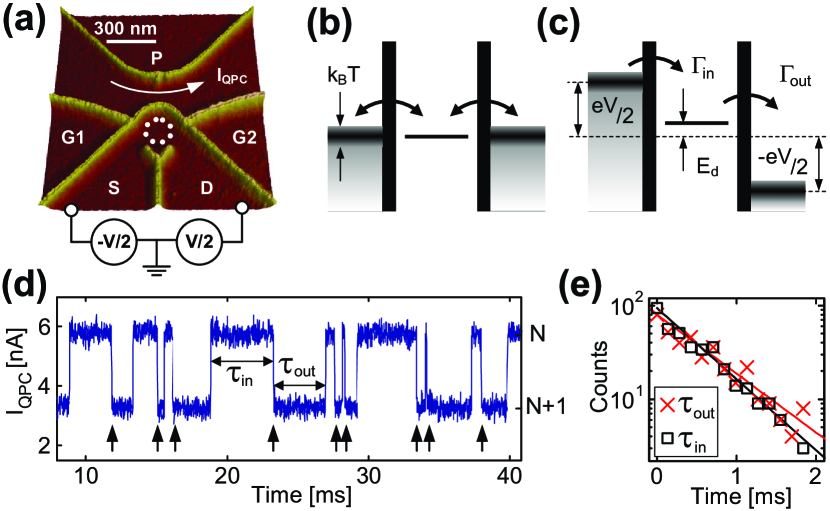
Figure 1: (a) AFM micrograph of the sample consisting of a QD connected to two contacts $S$ and $D$, and a nearby QPC. G1, G2 and P are lateral gates allowing the tuning of the tunnel coupling to the source $S$, the coupling to the drain $D$, and the conductance of the QPC. G1 and G2 are also used to tune the number of electrons in the QD. A symmetric bias voltage $V$ is applied between the source and the drain on the QD. (b-c) Scheme of the quantum dot in the case of equilibrium charge fluctuations (b), and non-equilibrium charge fluctuations (c). (d) Time trace of the current measured through the QPC corresponding to fluctuations of the charge of the dot between $N$ and $N+1$ electrons. The arrows indicate transitions where an electron is entering the QD from the source lead. (e) Probability density of the times $\tau_{in}$ and $\tau_{out}$ (see text) obtained from time traces similar to the one in (d). The lines correspond to the expected exponential dependence (see the text), where the tunneling rates are calculated from $1/\Gamma_{S(D)}=1/\Gamma_{in(out)}=\langle\tau_{in(out)}\rangle$.

Figure 1(a) shows the structure, fabricated on a GaAs-GaAlAs heterostructure containing a two-dimensional electron gas 34 nm below the surface (density $4.5\times 10^{15}$ m^-2, mobility 25 m²(Vs)^-1). An atomic force microscope (AFM) was used to oxidize locally the surface, thereby defining depleted regions below the oxide lines Held et al. (1999); Fuhrer et al. (2002). The measurements were performed in a ³He/⁴He dilution refrigerator with an electron temperature of about 350 mK, as determined from the width of thermally broadened Coulomb blockade resonances Kouwenhoven et al. (1997). The charging energy of the QD is $2.1$ meV and the mean level spacing is $200-300$ $\mu$eV. The conductance of the QPC, $G_{QPC}$, was tuned close to $0.25\times e^{2}/h$. We apply a dc bias voltage between source and drain of the QPC, $V_{QPC}=500$ $\mu$V, and measure the current through the QPC, $I_{QPC}$, which depends on the number of electrons $N$ in the QD.

In order to measure the current with a charge detector, one has to avoid that electrons travel back and forth between the dot and one lead or to the other lead due to thermal fluctuations [Fig. 1(b)]. This is achieved by applying a large bias voltage between source and drain, i.e. $|\!\>\pm eV/2-E_{d}|\gg k_{B}T$, where $E_{d}$ is the electrochemical potential of the dot and $V$ is the symmetrically applied bias, see Fig. 1(a, c). An example of a time trace of the QPC current in this configuration is shown in Fig. 1(d). The number of electrons in the QD fluctuates between $N$ and $N+1$. Since this trace corresponds to the non-equilibrium regime, we can attribute each transition $N\rightarrow N+1$ to an electron entering the QD from the source contact, and each transition $N+1\rightarrow N$ to an electron leaving the QD to the drain contact. The charge fluctuations in the QD correspond to a non-equilibrium process, and are directly related to the current through the dot Fujisawa et al. (2004). Due to Coulomb blockade, only one electron at a time can enter the QD, which allows to count electrons traveling through the system.

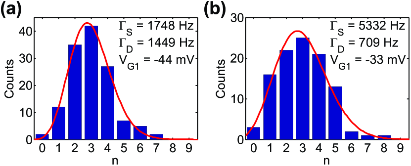
Figure 2: Statistical distribution of the number $n$ of electrons entering the QD during a given time $t_{0}$. The two panels correspond to two different values of the tunneling rates, obtained for different values of the gate voltage $V_{G1}$. The time $t_{0}$ is chosen in order to have the same mean value of number of events, $\langle n\rangle\approx 3$, for both graphs. We have checked that this choice does not affect the results. The line shows the theoretical distribution calculated from Eqs. (1) and (2). The tunneling rates are determined experimentally by the method described in Fig. 1(e), and no fitting parameters have been used for the theoretical curves.

The first application of electron counting in the non-equilibrium regime concerns the determination of the individual tunneling rates from the source to the QD, $\Gamma_{S}$, and from the QD to the drain, $\Gamma_{D}$. Previous experiments determining the individual tunneling rates involved more than two leads connected to the QD Leturcq et al. (2004). In the trace of Fig. 1(d), the time $\tau_{in}$ corresponds to the time it takes for an electron to enter the QD from the source contact, and $\tau_{out}$ to the time it takes for the electron to leave the QD to the drain contact. For independent tunneling events, the tunneling rates can be calculated from the average of $\tau_{in}$ and $\tau_{out}$ on a long time trace Schleser et al. (2004), $1/\Gamma_{S(D)}=1/\Gamma_{in(out)}=\langle\tau_{in(out)}\rangle$. To check that the tunneling events are indeed independent, we have compared the probability densities $p_{\tau_{in}}$ and $p_{\tau_{out}}$ with the expected exponential behavior $p(\tau_{in(out)})=\Gamma_{S(D)}\exp(-\Gamma_{S(D)}\tau_{in(out)})$. Figure 1(e) shows good agreement with our data. It is interesting to note that, in the case shown in Fig. 1(e), the QD is almost symmetrically coupled. We demonstrate here a very sensitive method to determine the symmetry of the coupling alternative to Ref. Rogge et al., 2005.

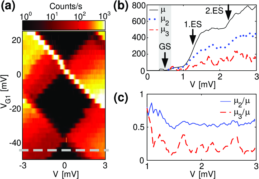
Figure 3: (a) Average number of electrons entering the QD, $\mu$, measured as a function of the gate voltage $V_{G1}$ and the bias voltage $V$. Far from the edges of the Coulomb blockade region, i.e. for $|\pm eV/2-E_{d}|\gg k_{B}T$, the fluctuations of $n$ are directly related to current fluctuations. The dashed line correspond to the cross-section shown in panel (b). (b) Three first moments of the fluctuations of $n$ as a function of the bias voltage $V$ and at a given gate voltage $V_{G1}=-44$ mV. The ground state (GS) as well as two excited states (ES) are clearly visible. The moments are scaled so that $\mu$ corresponds to the number of electrons entering the QD per second. In the gray region, the condition $|\pm eV/2-E_{d}|\gg k_{B}T$ is not valid, and the number of electrons entering the QD cannot be taken as the current flowing through the QD. The width of this region is $9\times k_{B}T/e\approx 300$ $\mu$V, determined from the width for which the Fermi distribution is between 0.01 and 0.99. (c) Normalized second and third moments as a function of the bias voltage $V$ and at a given gate voltage $V_{G1}=-44$ mV.

From traces similar to the one shown in Fig. 1(d), we can directly determine the statistical properties of sequential electron transport through the QD. We count the number $n$ of electrons entering the QD from the source contact during a time period $t_{0}$, i.e. the number of down-steps in Fig. 1(d) (see arrows). We obtain the distribution function of $n$ by repeating this counting procedure on $m=T/t_{0}$ independent traces, $T=0.5$ s being the total length of the time trace. The resulting distribution functions are shown for two different values of the tunneling rates in Figs. 2(a) and 2(b).

The FCS theory allows to determine the distribution function of the number $n$ of electrons traveling through a conductor Levitov et al. (1996):

$$P(n)=\int_{-\pi}^{\pi}\frac{d\chi}{2\pi}e^{-S(\chi)-n\chi},$$ (1)

where $S(\chi)$ is the generating function, which has been calculated for a single level QD for large bias voltage $|\pm eV/2-E_{d}|\gg k_{B}T$ Bagrets and Nazarov (2003):

$$\frac{S(\chi)}{t_{0}}=\left[\Gamma_{S}+\Gamma_{D}-\sqrt{\left(\Gamma_{S}-\Gamma_{D}\right)^{2}+4\Gamma_{S}\Gamma_{D}e^{-i\chi}}\right]$$ (2)

Here $\Gamma_{S}$ and $\Gamma_{D}$ are the effective tunneling rates, which take into account any possible spin degeneracy of the levels in the QD, and correspond to the tunneling rates we determine experimentally. We have calculated the theoretical distribution functions for the tunneling rates measured in the cases of Figs. 2(a) and 2(b) [solid lines]. The agreement with the experimental distribution is very good, in particular, given that no fitting parameters were used. Both graphs show a clear qualitative difference: Figure 2(b) shows a broader and more asymmetric distribution than Fig. 2(a). We will see later that this difference comes from the different asymmetries of the tunneling rates.

In order to perform a more quantitative analysis, we calculate the three first central moments given by $\mu=\langle n\rangle$, and $\mu_{i}=\langle(n-\langle n\rangle)^{i}\rangle$ for $i=$2,3, where $\langle...\rangle$ represents the mean over $T/t_{0}$ periods of length $t_{0}$. The first moment (mean) gives access to the mean current, $I=e\mu/t_{0}$, and the second central moment (variance) to the shot noise, $S_{I}=2e^{2}\mu_{2}/t_{0}$ (for $t_{0}$ much larger than the correlation time). We are also interested in the third central moment, $\mu_{3}$, which gives the asymmetry of the distribution function around its maximum (skewness). An important difference to previous measurements of the third cumulant is that our method can be used to extract any higher order cumulants. For the data presented here, the accuracy of the higher cumulants is limited by the short length of the time traces.

We first focus on the mean $\mu$ of the distribution. By measuring $\mu$ as a function of the voltage applied on gate G1 and the bias voltage $V$, we can construct the so-called Coulomb diamonds (see Fig. 3(a)). The Coulomb diamonds describe the charge stability of the QD, normally measured in standard transport experiments Kouwenhoven et al. (1997). Here, we present a novel way of measuring Coulomb blockade diamonds by time-resolved detection of the electrons using a non-invasive charge detector. We observe clear Coulomb blockade regions as well as regions of finite current. As we increase the bias voltage, we see steps in the current. The first step in Fig. 3(b) (see left arrow) corresponds to the alignment of the chemical potential of the source contact with the ground state in the QD, and the following steps with excited states in the QD. From the resolution of the Coulomb diamonds, we see that the sample is stable enough such that background charge fluctuations do not play a significant role Jung et al. (2004).

In addition to the mean, we have calculated the second and third central moments of the electron counting statistics. These two moments are shown in Fig. 3(b) for $V_{G1}=-44$ mV as a function of the bias voltage. The second moment (blue dotted line) reproduces the steps seen in the current. These two moments can be represented by their reduced quantities $\mu_{2}/\mu$ (known as the Fano factor) and $\mu_{3}/\mu$, as shown in Fig. 3(c). Both normalized moments are almost independent of the bias voltage, and correspond to a reduction compared to the values $\mu_{2}/\mu=\mu_{3}/\mu=1$ expected for classical fluctuations with Poissonian counting statistics. Super-poissonian noise Belzig (2005) is not expected in our configuration.

In a QD, one expects a reduction of the moments due to the fact that when one electron occupies the QD, a second electron cannot enter. This leads to correlations in the current fluctuations, and to a reduction of the noise. The reduction is maximal when the tunnel barriers are symmetric. For an asymmetrically coupled QD, the transport is governed by the slow barrier and the noise recovers the value for a single tunneling barrier. The normalized moments for a single level QD at large bias voltage can be expressed as a function of the asymmetry of the tunneling rates, $a=(\Gamma_{S}-\Gamma_{D})/(\Gamma_{S}+\Gamma_{D})$ Bagrets and Nazarov (2003):

$$\frac{\mu_{2}}{\mu}=\frac{1}{2}\left(1+a^{2}\right)\quad\text{and}\quad\frac{\mu_{3}}{\mu}=\frac{1}{4}\left(1+3a^{4}\right)\text{ .}$$ (3)

The second central moment recovers earlier calculations of the Fano factor in a QD Hershfield et al. (1993). We see in these equations that both moments are reduced for a symmetrically coupled QD (i.e. $a=0$), and tend to the Poissonian values for an asymmetrically coupled QD (i.e. $a=\pm 1$).

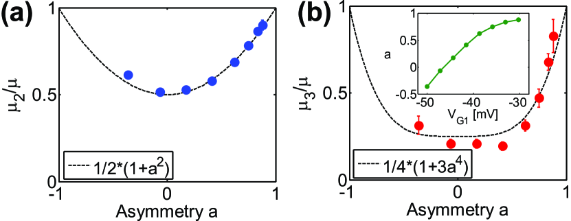
Figure 4: (a) Second and (b) third normalized central moments of the fluctuations of $n$ as a function of the asymmetry of the tunneling rates, $a=(\Gamma_{S}-\Gamma_{D})/(\Gamma_{S}+\Gamma_{D})$. To increase the resolution, each point at a given asymmetry is obtained by averaging over about $50$ points at a given voltage $V_{G1}$ and in a window of bias voltage $1.5<V<3$ mV. Error bars correspond to the standard error of this averaging process, and are of the size of the points if not shown. The dashed lines are the theoretical predictions given by Eqs. (3). No fitting parameters have been used, since the tunneling rates are fully determined experimentally (see Fig. 1(e) and text). Inset of (b): Variation of the asymmetry of the tunneling rates, $a$, as a function of $V_{G1}$.

Reduction of the second moment (shot noise) due to Coulomb blockade has already been reported in the case of asymmetrically coupled QDs Birk et al. (1995); Nauen et al. (2004). In these experiments, reduction of the shot noise occurs due to bias voltage dependent effective tunneling rates Hershfield et al. (1993). Here we report the reduction of the second, as well as the third moment for a fully controllable QD. In particular, we are able to continuously change the tunneling rates: by changing the gate voltage $V_{G1}$, we change the chemical potential in the QD, and also the asymmetry of the coupling by changing the opening of the source lead. The tunneling rates can be directly measured as described in Fig. 1(e), and the inset of Fig. 4(b) shows the variation of asymmetry with gate voltage in the region of interest. In Fig. 4(a) and 4(b), we show the normalized second and third central moments as a function of the asymmetry $a$. The experimental data follow the theoretical predictions given by Eqs. (3) very well. We note in particular that no fitting parameters have been used since the tunneling rates are determined experimentally.

Our ability to measure the counting statistics of electron transport relies on the high sensitivity of the QPC as a charge detector. The counting process that we demonstrate in this paper was not possible in previous experiments with the accuracy required for performing a statistical analysis Fujisawa et al. (2004). Given the bandwidth of our experimental setup, $\Delta f=30$ kHz, the method allows to measure currents up to $5$ fA, and we can measure currents as low as a few electrons per second, i.e., less than 1 aA. The low-current limitation is mainly given by the length of the time trace and the stability of the QD, and is well below what can be measured with conventional current meters. In addition, as we directly count electrons one by one, this measurement is not sensitive to the noise and drifts of the experimental setup. It is also an very sensitive way of measuring low current noise levels. Conventional measurement techniques are usually limited by the current noise of the amplifiers (typically $10^{-29}$ A²/Hz) de Picciotto et al. (1997); Birk et al. (1995); Nauen et al. (2004): here we demonstrate a measurement of the noise power with a sensitivity better than $10^{-35}$ A²/Hz.

In conclusion, we have measured current fluctuations in a semiconductor QD, using a QPC to detect single electron traveling through the QD. We show experimentally the reduction of the second and third moment of the distribution when the QD is symmetrically coupled to the leads. This ability to measure current fluctuations in a QD, as well as the very low noise level we demonstrate here, open new possibilities towards measuring electronic entanglement in quantum dot systems Loss and Sukhorukov (2000); Saraga and Loss (2003).