The Kardar-Parisi-Zhang equation in the weak noise limit:
Pattern formation and upper critical dimension

Abstract

We extend the previously developed weak noise scheme, applied to the noisy Burgers equation in 1D, to the Kardar-Parisi-Zhang equation for a growing interface in arbitrary dimensions. By means of the Cole-Hopf transformation we show that the growth morphology can be interpreted in terms of dynamically evolving textures of localized growth modes with superimposed diffusive modes. In the Cole-Hopf representation the growth modes are static solutions to the diffusion equation and the nonlinear Schrödinger equation, subsequently boosted to finite velocity by a Galilei transformation. We discuss the dynamics of the pattern formation and, briefly, the superimposed linear modes. Implementing the stochastic interpretation we discuss kinetic transitions and in particular the properties in the pair mode or dipole sector. We find the Hurst exponent H=(3-d)/(4-d) for the random walk of growth modes in the dipole sector. Finally, applying Derrick’s theorem based on constrained minimization we show that the upper critical dimension is d=4 in the sense that growth modes cease to exist above this dimension.

I Introduction

The large majority of natural phenomena are characterized by being out of equilibrium. This class includes turbulence in fluids, interface and growth problems, chemical reactions, processes in glasses and amorphous systems, biological processes, and even aspects of economical and sociological structures.

As a consequence much of the focus of modern statistical physics, soft condensed matter, and biophysics has shifted towards such systems Nelson (2003); Chaikin and Lubensky (1995). Drawing on the case of static and dynamic critical phenomena in and close to equilibrium, where scaling and the concept of universality have successfully served to organize our understanding and to provide a variety of calculational tools Binney et al. (1992), a similar strategy has been advanced towards the much larger class of nonequilibrium phenomena with the purpose of elucidating scaling properties and more generally the morphology or pattern formation in a driven nonequilibrium system Chaikin and Lubensky (1995); Cross and Hohenberg (1994).

There is a particular interest in the scaling properties and general morphology of nonequilibrium models Cross and Hohenberg (1994); Barabasi and Stanley (1995). Here the Kardar-Parisi-Zhang (KPZ) equation has played a prominent and paradigmatic role. The KPZ equation describes aspects of the nonequilibrium kinetic growth of a noise-driven interface and provides a simple continuum model of an open driven nonlinear system exhibiting scaling and pattern formation Kardar et al. (1986); Medina et al. (1989).

The KPZ equation for the time evolution of the height field $h({\bf r},t)$ has the form

$$\frac{\partial h}{\partial t}=\nu{\bm{\nabla}}^{2}h+\frac{\lambda}{2}{\bm{\nabla}}h\cdot{\bm{\nabla}}h-F+\eta,$$ (1)

$$\langle\eta({\bf r},t)\eta({\bf r}^{\prime},t^{\prime})\rangle=\Delta\delta^{d}({\bf r}-{\bf r}^{\prime})\delta(t-t^{\prime}).$$ (2)

Here the damping coefficient or surface tension $\nu$ characterizes the linear diffusion term, the parameter $\lambda$ controls the strength of the nonlinear growth term, $F$ is a constant imposed drift term, and $\eta$ a locally correlated white Gaussian noise modelling the stochastic nature of the drive or environment; the noise correlations are characterized by the noise strength $\Delta$ Krug (1997); Barabasi and Stanley (1995); Krug et al. (1992); Family (1990); Halpin-Healy and Zhang (1995).

In terms of the vector slope field

$${\bf u}={\bm{\nabla}}h,$$ (3)

the KPZ equation maps onto the Burgers equation driven by conserved noise Forster et al. (1976, 1977); E and Vanden-Eijnden (2000); Woyczynski (1998)

$$\frac{\partial{\bf u}}{\partial t}=\nu{\bm{\nabla}}^{2}{\bf u}+\lambda({\bf u}\cdot{\bm{\nabla}}){\bf u}+{\bm{\nabla}}\eta.$$ (4)

In the deterministic case for $\eta=0$ the Burgers equation has been used to study irrotational fluid motion and turbulence Burgers (1929, 1974); Saffman (1968); Jackson (1990); Whitham (1974) and also as a model for large scale structures in the universe Zeldovitch (1972).

In a series of papers we have analyzed the one dimensional noisy Burgers equation for the slope field of a growing interface. In Ref. Fogedby (1998a) we discussed as a prelude the noiseless Burgers equation Burgers (1929, 1974) in terms of its nonlinear soliton or shock wave excitations and performed a linear stability analysis of the superimposed diffusive mode spectrum. This analysis provided a heuristic picture of the damped transient pattern formation. As a continuation of previous work on the continuum limit of a spin representation of a solid-on-solid model for a growing interface Fogedby et al. (1995), we applied in Ref. Fogedby (1998b) the Martin-Siggia-Rose formalism Martin et al. (1973) in its path integral formulation Baussch et al. (1976); Janssen (1976); DeDominicis and Peliti (1978) to the noisy Burgers equation Forster et al. (1976, 1977) and discussed in the weak noise limit the growth morphology and scaling properties in terms of nonlinear soliton or domain wall excitations with superimposed linear diffusive modes. In Ref. Fogedby (1999a) we pursued a canonical phase space approach based on the weak noise saddle point approximation to the Martin-Siggia-Rose functional or, alternatively, the Freidlin-Wentzel symplectic approach to the Fokker-Planck equation Freidlin and Wentzel (1998); Graham (1989). This method provides a dynamical system theory point of view Lichtenberg and Lieberman (1983); Ott (1993); Schuster (1989) to weak noise stochastic processes and yields direct access to the probability distributions for the noisy Burgers equation; brief accounts of the above works has appeared in Refs. Fogedby (1998c, 1999b). Further work on the scaling properties and a numerical investigation of domain wall collisions has appeared in in Refs. Fogedby (2001a, b); Fogedby and Brandenburg (2002); Fogedby (2002a, b). A detailed summary and further developments have been given in an extensive paper Fogedby (2003a).

In the present work we address the KPZ equation for a growing interface in arbitrary dimensions. Applying an extended form of the canonical weak noise approach in order to incorporate multiplicative noise and drawing from the insight gained by the analysis of the 1D noisy Burgers equation, we identify the localized growth modes for the KPZ equation. The growth modes are spherically symmetric and are equivalent to the domain walls or solitons identified in the 1D case. The growth modes propagate and a dilute gas of modes constitute a dynamical network accounting for the kinetic growth of the interface.

We also consider the issue of an upper critical dimension for the KPZ equation. The KPZ equation lives at a critical point, conforms to the dynamical scaling hypothesis Barabasi and Stanley (1995); Family (1986, 1990) and is characterized by the scaling exponents $z$ and $\zeta$ Halpin-Healy and Zhang (1995); Krug (1997). Dynamic renormalization group calculations yield $d=2$ as lower critical dimension Forster et al. (1977); Medina et al. (1989). In addition to the scaling properties in the rough phase, characterized by a strong coupling fixed point, a major open problem remains the existence of an upper critical dimension Wiese (1998); Lässig and Kinzelbach (1997); Colaiori and Moore (2001a). In the present context we interpret the upper critical dimension as the dimension beyond which the growth modes cease to exist. On the basis of a numerical analysis and an exact argument based on Derrick’s theorem Derrick (1964) we propose that $d=4$ is the upper critical dimension for the KPZ equation.

The paper is organized in the following way. To bring the reader up to date we review in Sec. II the KPZ equation with emphasis on the scaling properties. In Sec. III we summarize the weak noise approach including an extension to the case of multiplicative noise in order to treat the KPZ equation in the Cole-Hopf representation. In Sec. IV we address the KPZ equation and the associated noisy Burgers and Cole-Hopf equations within the weak noise scheme and derive the fundamental deterministic field equations governing the weak noise behavior. In Sec. V we turn to the solutions of the field equations. As a prelude we review the solutions in the 1D case and then turn to the KPZ equation in its Cole-Hopf representation in higher dimensions. In Sec. VI we form a dynamical network of growth modes accounting for the growth morphology of the KPZ equation. We establish a field theory based on the picture of the growth modes as charged monopoles. Finally, we discuss briefly the superimposed linear mode spectrum. In Sec. VII we turn to the stochastic interpretation and discuss kinetic transitions and in particular the anomalous diffusion and scaling in the dipole sector. In Sec. VIII we discuss the issue of the upper critical dimension and present, using Derrick’s theorem based on constrained minimization, an algebraic proof of the upper critical dimension being equal to four. Sec. IX is devoted to a summary, a list of open problems, and a conclusion. In appendix A we consider the application of the weak noise method to Brownian motion and the overdamped oscillator. Aspects of the present work has appeared in Ref. Fogedby (2005).

II The KPZ equation

The KPZ equation (1) was proposed as a model for the kinetic nonequilibrium growth of an interface driven by noise Kardar et al. (1986); Medina et al. (1989); Barabasi and Stanley (1995). Although the equation only describes limited aspects of true interface growth and, for example, ignores surface diffusion Krug (1997), the equation has achieved an important and paradigmatic status in the theory of nonequilibrium processes Halpin-Healy and Zhang (1995). In many regards the KPZ equation serves as a prototype continuum model for nonequilibrium processes in much the same way as the Ginzburg-Landau functional in, for example, the context of critical phenomena Binney et al. (1992); Chaikin and Lubensky (1995).

II.1 General Properties

From a structural point of view the KPZ equation (1) has the form of a noise-driven diffusion equation with a simple nonlinear term added. Whereas the diffusion term $\nu{\bm{\nabla}}^{2}h$ gives rise to a local flattening or relaxation of the interface, corresponding to a surface tension, the crucial nonlinear term $(\lambda/2){\bm{\nabla}}h\cdot{\bm{\nabla}}h$ accounts for the lateral growth of the interface Barabasi and Stanley (1995). In that sense the KPZ equation is a genuine kinetic equation describing a nonequilibrium process in the sense that the drift term $\nu{\bm{\nabla}}^{2}h+(\lambda/2){\bm{\nabla}}h\cdot{\bm{\nabla}}h-F$ cannot be derived from an effective free energy. The noise drives the height field into a stationary state whose distribution is not known in detail except in 1D, where it is independent of $\lambda$ and given by Huse et al. (1985); Halpin-Healy and Zhang (1995)

$$P_{0}(h)\propto\exp\left[-\frac{\nu}{\Delta}\int dx~{}({\bm{\nabla}}h)^{2}\right].$$ (5)

In the linear case for $\lambda=0$ the KPZ equation (1) reduces to the Edwards-Wilkinson equation (EW) Edwards and Wilkinson (1982)

$$\frac{\partial h}{\partial t}=-\frac{1}{2}\frac{\delta{\cal F}}{\delta h}-F+\eta~{},~{}~{}{\cal F}=\nu\int d^{d}x~{}({\bm{\nabla}}h)^{2},$$ (6)

which in a comoving frame with velocity $-F$ describes an interface in thermal equilibrium at temperature $T=\Delta$ with stationary Boltzmann distribution given by Eq. (5). In the EW case we also have access to the time-dependent distribution. Expanding the height field on a plane wave basis, $h({\bf r})=\int d^{d}x~{}h_{\bf k}\exp(i{\bf kr})$ and introducing the diffusive mode frequency $\omega_{\bf k}=\nu{\bf k}^{2}$ we obtain for the transition probability from an initial profile $h_{\bf k}^{0}$ to a final profile $h_{\bf k}$ in time $T$ Krug (1997)

$$P(h_{k},T)\propto$$

$$\left[-\frac{\nu}{\Delta}\int\frac{d^{d}k}{(2\pi)^{d}}~{}k^{2}\frac{|h_{\bf k}-h_{\bf k}^{0}\exp(-\omega_{\bf k}T)|^{2}}{1-\exp(-2\omega_{\bf k}T)}\right],~{}~{}$$ (7)

and, for example, the height correlation function

$$\langle hh\rangle({\bf k},\omega)=\frac{\Delta}{\omega^{2}+(\nu k^{2})^{2}},$$ (8)

with a Lorentzian line shape controlled by the diffusive poles at $\omega=\pm i\nu k^{2}$; see also Ref. Majaniemi et al. (1996).

Averaging the KPZ equation in a state at times where transients have died out, we obtain

$$\frac{d\langle h\rangle}{dt}=(\lambda/2)\langle{\bm{\nabla}}h\cdot{\bm{\nabla}}h\rangle-F,$$ (9)

showing that the nonlinear term gives rise to nonequilibrium growth determined by the magnitude of $\langle{\bm{\nabla}}h\cdot{\bm{\nabla}}h\rangle$; note that choosing $F$ to balance the nonlinear term, i.e., $F=(\lambda/2)\langle{\bm{\nabla}}h\cdot{\bm{\nabla}}h\rangle$, is equivalent to choosing a comoving frame in which $d\langle h\rangle/dt=0$.

In addition to being invariant under time and space translations, the KPZ equation (1) is also invariant subject to the nonlinear Galilei transformation:

$${\bf r}\rightarrow{\bf r}-\lambda{\bf u}^{0}t,$$ (10)

$$h\rightarrow h+{\bf u}^{0}\cdot{\bf r},$$ (11)

$$F\rightarrow F+(\lambda/2){\bf u}^{0}\cdot{\bf u}^{0}.$$ (12)

Hence, the transformation to a moving frame with velocity $\lambda{\bf u}^{0}$ is absorbed by adding a constant slope term ${\bf u}^{0}\cdot{\bf r}$ to the height field $h$ and shifting the constant drift term by $(\lambda/2){\bf u}_{0}^{2}$. Note that the invariance is associated with the nonlinear parameter $\lambda$ which enters as a structural constant in the Galilei group transformation; in the EW case this invariance is absent.

The KPZ equation is characterized by the parameters $\nu$, $\lambda$, $F$, and $\Delta$ of dimension $[\nu]=L^{2}/T$, $[\lambda]=L/T$, $[F]=L/T$, and $[\Delta]=L^{d+2}/T$. By transforming to a comoving frame $h\rightarrow h-Ft$ we can absorb the drift $F$ for a given growth morphology and from the remaining dimensionfull parameters form the dimensionless parameter $\Delta\lambda^{d}/\nu^{d+1}$. Consequently, the weak noise limit $\Delta\rightarrow 0$ is equivalent to the weak coupling limit $\lambda\rightarrow 0$ (or the limit of large damping $\nu\rightarrow\infty$). In Fig. 1 we have in 2D depicted a growing interface.

Figure 1: We depict a growing interface in 2D (arbitrary units).

II.2 Burgers equation and Cole-Hopf equation

The paradigmatic importance of the KPZ equation stems from the fact that it in addition to describing nonequilibrium surface growth also is associated with the theory of turbulence via its equivalence to the noisy Burgers equation (4). Moreover, by means of the nonlinear Cole-Hopf tranformation Cole (1951); Hopf (1950); Medina et al. (1989)

$$w=\exp\left[\frac{\lambda}{2\nu}h\right],$$ (13)

the KPZ equation takes the form of a linear diffusion equation driven by multiplicative noise, denoted here the Cole-Hopf equation,

$$\frac{\partial w}{\partial t}=\nu{\bm{\nabla}}^{2}w-\frac{\lambda}{2\nu}wF+\frac{\lambda}{2\nu}w\eta.$$ (14)

In the absence of noise Eq. (14) becomes the linear diffusion equation and is readily analyzed, thus allowing a discussion of the KPZ and Burgers equations in the deterministic case Medina et al. (1989); Woyczynski (1998). In the noisy case a path integral representation of the solution of Eq. (14) maps the Cole-Hopf equation and thus the KPZ equation onto a model of a directed polymer with line tension $1/4\nu$ in a quenched random potential $(\lambda/2\nu)\eta({\bf r},t)$. The disordered directed polymer model is a toy model within the spin glass literature and has been analyzed by means of the replica method and Bethe ansatz techniques Kardar (1987); Halpin-Healy and Zhang (1995).

The Galilean invariance of the KPZ equation is for the Burgers equation (4) and the Cole-Hopf equation (14) supplemented by the transformations

$${\bf u}\rightarrow{\bf u}+{\bf u}^{0},$$ (15)

$$w\rightarrow w\exp\left[\left(\lambda/2\nu\right){\bf u}^{0}\cdot{\bf r}\right],$$ (16)

i.e., the slope field is shifted by ${\bf u}^{0}$ and the Cole-Hopf field by the multiplicative factor $\exp[(\lambda/2\nu){\bf u}^{0}\cdot{\bf r}]$.

II.3 Scaling properties

The KPZ equation conforms to the dynamical scaling hypothesis with long time-large distance height correlations Barabasi and Stanley (1995); Family and Vicsek (1985)

$$\langle hh\rangle({\bf r},t)=r^{2\zeta}\Phi(t/r^{z}),$$ (17)

characterized by the roughness exponent $\zeta$, dynamical exponent $z$, and scaling function $\Phi$. Consequently, most theoretical efforts have addressed the scaling issues. Based on i) perturbative dynamic renormalization group (DRG) calculations in combination with the scaling law

$$\zeta+z=2,$$ (18)

following from Galilean invariance, and the known stationary height distribution in 1D given by Eq. (5) Medina et al. (1989); Huse et al. (1985); Wiese (1997), ii) the mapping of the KPZ equation onto directed polymers in a quenched environment and ensuing replica calculations Halpin-Healy and Zhang (1995); Kardar (1987), iii) mode coupling calculations Schwartz and Edwards (1992); Bouchaud and Cates (1993); Doherty et al. (1994); Moore et al. (1995), iv) operator expansion methods Lässig (1998), and v) numerical calculations Marinari et al. (2000, 2002); New ; Beccaria and Curci (1994), the following picture has emerged.

In 1D the interface is rough and characterized by a perturbatively inaccessible strong coupling fixed point with scaling exponents $z=3/2$ and $\zeta=1/2$, following from the stationary distribution in combination with the scaling law. Above the lower critical dimension $d=2$ a DRG calculation in $\epsilon=d-2$ predicts a kinetic transition line between a smooth phase characterized by a weak coupling fixed point at $\lambda=0$ with exponents $z=2$ and $\zeta=(2-d)/2$ and a rough phase characterized by a poorly understood strong coupling fixed point. On the transition line $z=2$ and $\zeta=0$ Lässig (1995); Wiese (1998). Based on numerics the following expressions for $z$ have been proposed: $z_{\text{KK}}=2(d+2)/(d+3)$ Kim and Kosterlitz (1989) and $z_{\text{WK}}=(2d+1)/(d+1)$ Wolf and Kertész (1997). Both $z_{\text{KK}}$ and $z_{\text{WK}}$ agree with $z=3/2$ in $d=1$; for $d\rightarrow\infty$ we have $z\rightarrow 2$, corresponding to a smooth phase at an infinite upper critical dimension. An operator expansion method Lässig (1998) yields $z_{\text{L}}=4d/(2d+1)$ for $d>1$ and $z\rightarrow 2$ for $d\rightarrow\infty$. The scaling properties of the KPZ equation is summarized in Fig. 2 in a plot of the renormalized coupling strength $g=\lambda^{2}\Delta/\nu^{3}$ versus spatial dimension.

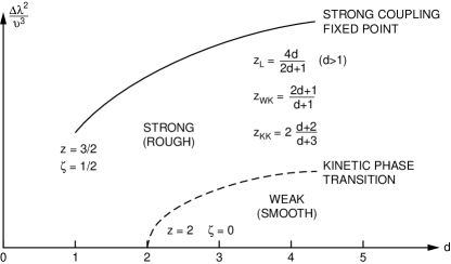
Figure 2: We summarize the scaling properties of the KPZ equation in a plot of the renormalized coupling constant (the fixed point value) $\Delta\lambda^{2}/\nu^{3}$ versus the dimension $d$ of the system. Below $d=2$ the scaling properties are determined by the strong coupling fixed. Above $d=2$ the system exhibits a kinetic phase transition from a weak coupling phase to a strong coupling phase. We have also indicated three conjectures for the exponent $z$: The operator expansion conjecture $z_{L}$ by Lässig Lässig (1998) and the conjectures based on numerics, $z_{WK}$ by Wolf and Kertész Wolf and Kertész (1997) and $z_{KK}$ by Kim and Kosterlitz Kim and Kosterlitz (1989).

Whereas $d=2$ constitutes the lower critical dimension permitting a loop expansion in powers of $\epsilon$, the issue of an upper critical dimension has been much debated. Mode coupling approaches yield an upper critical dimension $d=4$ with a possible glassy behavior above 4 Moore et al. (1995); Bhattacharjee (1998); Colaiori and Moore (2001a, b). Loop expansion to all orders in $\epsilon$ supported by an exact evaluation of the beta-function in a Callen-Symanzik renormalization group scheme associates the upper critical dimension with a mathematical singularity Lässig and Kinzelbach (1997); Wiese (1998).

Two outstanding issues thus remain as regard the scaling properties of the KPZ equation: The upper critical dimension and the properties of the strong coupling fixed point above $d=1$, i.e., the scaling exponents and scaling function. There is, moreover, the more general question of the deeper mechanism behind the stochastic growth morphology. In that respect the KPZ equation shares its strong coupling features with another notable problem in theoretical physics: Turbulence.

Since the DRG in its perturbative form as an expansion about the linear theory fails to yield insight into the strong coupling features there clearly is a need for alternative systematic methods. Here we should like to emphasize that both the mode coupling approaches Moore et al. (1995); Doherty et al. (1994); Colaiori and Moore (2001a, b); Bouchaud and Cates (1993); Bhattacharjee (1998) and operator expansion methods Lässig (1998) do not qualify as being systematic. The mode coupling approach is based on a truncation procedure ignoring vertex corrections and thus violating Galilean invariance which is essential in delimiting the KPZ universality class. The operator product expansion imposes an ad hoc mathematically motivated operator structure.

III The weak noise method

The weak noise method is based on an asymptotic weak noise approximation to a general Langevin equation driven by Gaussian white noise. The method dates back to Onsager Onsager and Machlup (1953); Machlup and Onsager (1953) and has since reappeared as the Freidlin-Wentzel theory of large deviations Freidlin and Wentzel (1998); Graham (1989) and as the weak noise saddle point approximation to the functional Martin-Siggia-Rose scheme Martin et al. (1973); Baussch et al. (1976); Janssen (1976); DeDominicis and Peliti (1978). The method known also as the eikonal approximation has, moreover, been used in the context of thermally activated escape Graham and Tél (1984a, b); Graham et al. (1985); Graham (1989); Dykman (1990); Bray and McKane (1989); Maier and Stein (1996, 2001); Aurell and Sneppen (2002). The weak noise or canonical phase space method has been discussed in Ref. Fogedby (1999a). In the present context we need a generalization of the method in order to accommodate multiplicative noise and therefore review and extend the method below.

III.1 General properties

The point of departure is the generic Langevin equations for a set of stochastic variables $w_{n}$, $n=1,\cdots N$, driven by white Gaussian noise Stratonovich (1963)

$$\frac{dw_{p}}{dt}=-\frac{1}{2}F_{p}-\frac{\Delta}{2}G_{mn}\nabla_{m}G_{pn}+G_{pn}\eta_{n},$$ (19)

$$\langle\eta_{n}\eta_{m}\rangle(t)=\Delta\delta_{nm}\delta(t),$$ (20)

where $F_{n}(w_{q})$ is the drift, $G_{nm}(w_{q})$ is accounting for multiplicative noise, $\nabla_{n}=\partial/\partial w_{n}$, and $\Delta$ is the explicit noise strength; sums are performed over repeated indices. In the case of multiplicative noise with $G$ depending on $w$ this is the Stratonovich formulation. In the Ito formulation the compensating drift term $G\nabla G$ is absent corresponding to the application of the Ito differentiation rules Risken (1989); Reimann (2002). Note that in the case of i) additive noise, i.e., $G$ independent of $w$ or ii) to leading order in $\Delta$ the Ito and Stranovich formulations are equivalent. The generic Langevin equation (19) driven by white noise encompasses with appropriate choices of $F$ and $G$ all white noise driven continuous Markov processes.

On the deterministic level the corresponding Fokker-Planck equation for the probability distribution $P(w_{n},t)$ has the form Stratonovich (1963)

$$\frac{\partial P}{\partial t}=\frac{1}{2}\nabla_{n}[F_{n}+\Delta\nabla_{m}K_{mn}]P,$$ (21)

where the symmetrical noise matrix is given by

$$K_{pm}(w_{q})=G_{pn}(w_{q})G_{mn}(w_{q}).$$ (22)

In complete analogy with the WKB approach in quantum mechanics Landau and Lifshitz (1959a), $\Psi\propto\exp[iS/\hbar]$, relating the wave function $\Psi$ to the classical action $S$ evaluated on the basis of the classical Hamilton equations of motion, it is useful to capture weak noise effects and relate the stochastic problem to a scheme based on classical equations of motion by means of a weak noise WKB approximation to the Fokker-Planck equation (21). Thus introducing the Wentzel-Kramers-Brillouin (WKB) ansatz

$$P(w_{n},t)\propto\left[-\frac{S(w_{n},t)}{\Delta}\right],$$ (23)

we obtain to leading order in the noise strength $\Delta$ the Hamilton-Jacobi equation Landau and Lifshitz (1959a); Goldstein (1980)

$$\frac{\partial}{\partial t}+H=0~{},~{}~{}p_{n}=\nabla_{n}S,$$ (24)

with Hamiltonian

$$H=-\frac{1}{2}p_{n}F_{n}+\frac{1}{2}K_{nm}p_{n}p_{m}.$$ (25)

The Hamiltonian equations of motion follow from $dw_{n}/dt=\partial H/\partial p_{n}$ and $dp_{n}/dt=-\partial H/\partial w_{n}$,

$$\frac{dw_{n}}{dt}=-\frac{1}{2}p_{n}F_{n}+K_{nm}p_{m},$$ (26)

$$\frac{dp_{n}}{dt}=\frac{1}{2}p_{m}\nabla_{n}F_{m}-\frac{1}{2}p_{m}p_{q}\nabla_{n}K_{mq},$$ (27)

determining classical orbits on the energy surfaces given by $H$ in a classical phase space $(\{w_{n}\},\{p_{n}\})$. Finally, the action $S$ is given by

$$S(w_{n},T)=\int^{w_{n},T}_{w_{n}^{\text{i}},0}dt~{}p_{n}\frac{dw_{n}}{dt}-HT,$$ (28)

yielding according to Eq. (23) the transition probability. By means of the equation of motion (26) the action can be reduced to the form

$$S(w_{n},T)=\frac{1}{2}\int^{w_{n},T}_{w_{n}^{\text{i}},0}dt~{}K_{nm}p_{n}p_{m}.$$ (29)

The weak noise scheme bears the same relationship to stochastic fluctuations as the WKB approximation in quantum mechanics, associating the phase of the wave function with the action of the corresponding classical orbit Landau and Lifshitz (1959a). In addition to providing a classical orbit picture of stochastic fluctuations and thus allowing the use of dynamical system theory Arnold (1983); Jackson (1990); Lichtenberg and Lieberman (1983); Reichl (1987); Scott (1999); Schuster (1989), the method also yields the Arrhenius factor $P\propto\exp(-S/\Delta)$ for a kinetic transition from $w_{n}^{\text{i}}$ to $w_{n}$ during the transition time $T$. Here the action $S$ serves as the weight in the same manner as the energy $E$ in the Boltzmann factor $P\propto\exp(-\beta E)$, $\beta=1/kT$, for equilibrium processes.

In the weak noise scheme the stochastic Langevin equation (19) is replaced by the deterministic equation of motion (26) for $w_{n}$ which together with the equation of motion (27) for the canonically conjugate noise variable $p_{n}$ determine orbits lying on the constant energy manifolds $H=\text{const.}$ in a canonical phase space spanned by $w_{n}$ and $p_{n}$. Determining a specific orbit from $w_{n}^{\text{i}}$ to $w_{n}$ in time $T$ by solving the equations of motion (26) and (27) with $p_{n}$ as a slaved variable, evaluating the action (28), then yields the (unnormalized) transition probability in Eq. (23).

A stationary distribution of the Fokker-Planck equation (21) is given by

$$P_{0}(w_{n})=\lim_{T\rightarrow\infty}P(w_{n},T),$$ (30)

satisfying $(1/2)\nabla_{n}[F_{n}+\Delta\nabla_{m}K_{mn}]P=0$. Within the dynamical system theory framework to leading asymptotic order in $\Delta$ this implies that $S(w_{n},T)\rightarrow S_{0}(w_{n})$ for fixed final configuration $w_{n}$, i.e., $P_{0}\propto\exp[-S_{0}/\Delta]$. To attain the stationary limit an orbit from an initial configuration $w_{n}^{\text{i}}$ to a final configuration $w_{n}$ traversed in time $T\rightarrow\infty$ must (i) pass through a saddle point and (ii) in the limit lie on a zero-energy manifold $H=0$. The zero-energy manifold is in general composed of two submanifolds intersecting at the saddle point. The transient or noiseless submanifold $p=0$, yielding $H=0$ and consistent with the equations of motion, corresponds to the transient motion determined by the noiseless equation of motion $dw_{n}/dt=-(1/2)p_{n}F_{n}$. The stationary or noisy submanifold determined by the orthogonality condition $p_{n}[K_{nm}p_{m}-F_{n}]=0$, corresponds to the stationary motion. The loss of memory and Markovian behavior result from the infinite waiting time at the saddle point; for details see e.g. Ref. Fogedby (1999a).

We, moreover, note that the weak noise scheme has a symplectic structure with Poisson bracket algebra Landau and Lifshitz (1959b); Goldstein (1980)

$$\{w_{n},p_{m}\}=\delta_{nm},~{}~{}\{w_{n},w_{m}\}=\{p_{n},p_{m}\}=0,$$ (31)

and Hamiltonian equations of motion

$$\frac{dw_{n}}{dt}=\{w_{n},H\}~{},~{}~{}\frac{dp_{n}}{dt}=\{p_{n},H\}.$$ (32)

In Fig. 3 we have depicted the generic phase space structure in the case where the system possesses a stationary state.

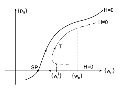
Figure 3: The $(\{w_{n}\},\{p_{n}\})$ phase space with a finite-time orbit from $\{w_{n}^{i}\}$ to $\{w_{n}\}$ in time $T$ on a $H\neq 0$ energy manifold, yielding the transition probability, and an infinite-time stationary orbit to $\{w_{n}\}$ passing through the saddle point SP and lying on the $H=0$ energy manifold.

The purpose of the weak noise scheme is twofold. On the one hand, it provides an alternative way of discussing stochastic phenomena in terms of an equivalent deterministic scheme based on canonical equations of motion, orbits in phase space, and the ensuing dynamical system theory concepts. The scheme, on the other hand, also provides a calculational tool in determining the transition probabilities and ensuing correlations. It is also important to keep in mind that although the starting point is a weak noise approximation the scheme, like WKB in quantum mechanics, is nonperturbative and is thus capable of accounting at least qualitatively for strong noise effects. This point of view was stressed by Coleman in the context of quantum field theories Coleman (1977).

This completes our general discussion of the weak noise approach. As an illustration we consider in appendix A the application of the method to two systems with a single degree of freedom: (i) random walk and (ii) the overdamped oscillator. See also an application to a nonlinear finite-time-singularity model in Refs. Fogedby and Poukaradze (2002); Fogedby (2003b) and to an extended system, the noise-driven Ginzburg-Landau model, in Refs Fogedby et al. (2003, 2004).

IV The KPZ equation for weak noise

Here we apply the weak noise method to the KPZ equation, the corresponding noisy Burgers equation and Cole-Hopf equation.

IV.1 The KPZ case

Adapting the KPZ equation (1) to the weak noise scheme we make the assignment: $w_{n}(t)\rightarrow h({\bf r},t),p_{n}(t)\rightarrow\tilde{p}({\bf r},t),K_{nm}\rightarrow\delta^{d}({\bf r}-{\bf r}^{\prime}),F_{n}\rightarrow-2\left[\nu{\bm{\nabla}}^{2}h+(\lambda/2){\bm{\nabla}}h\cdot{\bm{\nabla}}h-F\right]$. Here the index $n$ becomes the spatial coordinate ${\bf r}$. We thus obtain the KPZ Hamiltonian density

$${\cal H}^{\text{KPZ}}=\tilde{p}\left[\nu{\bm{\nabla}}^{2}h+\frac{\lambda}{2}{\bm{\nabla}}h\cdot{\bm{\nabla}}h-F+\frac{1}{2}\tilde{p}\right],$$ (33)

and the canonical field equations

$$\frac{\partial h}{\partial t}=\nu{\bm{\nabla}}^{2}h+\frac{\lambda}{2}{\bm{\nabla}}h\cdot{\bm{\nabla}}h-F+\tilde{p},$$ (34)

$$\frac{\partial\tilde{p}}{\partial t}=-\nu{\bm{\nabla}}^{2}\tilde{p}+\lambda{\bm{\nabla}}\tilde{p}\cdot{\bm{\nabla}}h+\lambda\tilde{p}\nabla^{2}h.$$ (35)

The reduced action and transition probability are given by

$$S^{\text{KPZ}}(h,T)=\frac{1}{2}\int^{h,T}d^{d}xdt~{}\tilde{p}({\bf r},t)^{2},$$ (36)

$$P^{\text{KPZ}}(h,T)\propto\exp\left[-\frac{S^{\text{KPZ}}(h,T)}{\Delta}\right].$$ (37)

The height field $h$ and noise field $\tilde{p}$ are canonically conjugate variables in the canonical phase space $(\{h({\bf r}\},\{\tilde{p}({\bf r}\})$,

$$\{h({\bf r}),\tilde{p}({\bf r}^{\prime})\}=\delta^{d}({\bf r}-{\bf r}^{\prime}).$$ (38)

We, moreover, have the generators of time translation and space translation, i.e., energy and momentum,

$$H^{\text{KPZ}}=\int d^{d}x~{}{\cal H}^{\text{KPZ}}~{},~{}~{}\{h,H^{\text{KPZ}}\}=\frac{\partial h}{\partial t},~{}~{}$$ (39)

$${\bm{\Pi}}^{\text{KPZ}}=\int d^{d}x~{}h{\bm{\nabla}}\tilde{p}~{},~{}~{}\{h,{\bm{\Pi}}^{\text{KPZ}}\}={\bm{\nabla}}h.$$ (40)

The Galilean invariance of the KPZ equation (1) implies that the noise field $\tilde{p}$ is invariant; this also follows from the invariance of the action in Eq.(36).

This completes the formal application of the weak noise scheme to the KPZ equations. The resulting classical field theory must then be addressed in order to eventually evaluate transition probabilities and correlations.

IV.2 The Cole-Hopf case

The Cole-Hopf equation (14) is obtained by applying the nonlinear Cole-Hopf transformation (13) to the KPZ equation (1). The Cole-Hopf equation is driven by multiplicative noise and most work has been based on the mapping to directed polymers in a random medium Halpin-Healy and Zhang (1995). In the present context it turns out that a weak noise representation provides a particular symmetric formulation. Hence, making the assignment, $w_{n}(t)\rightarrow w({\bf r},t),p_{n}(t)\rightarrow p({\bf r},t),K_{nm}\rightarrow(\lambda/2\nu)^{2}w^{2}\delta^{d}({\bf r}-{\bf r}^{\prime}),F_{n}\rightarrow-2\left[\nu{\bm{\nabla}}^{2}w-(\lambda/2\nu)wF\right]$, we obtain the Cole-Hopf Hamiltonian density

$${\cal H}^{\text{CH}}=p[\nu{\bm{\nabla}}^{2}-\nu k^{2}]w+\frac{1}{2}k_{0}^{2}(wp)^{2},$$ (41)

where we have introduced two characteristic inverse length scales

$$k=\left(\frac{\lambda F}{2\nu^{2}}\right)^{1/2}~{},~{}~{}k_{0}=\frac{\lambda}{2\nu}.$$ (42)

The field equations are given by

$$\frac{\partial w}{\partial t}=\nu[{\bm{\nabla}}^{2}w-k^{2}w]+k_{0}^{2}w^{2}p,$$ (43)

$$\frac{\partial p}{\partial t}=-\nu[{\bm{\nabla}}^{2}p-k^{2}p]-k_{0}^{2}p^{2}w,$$ (44)

and the reduced action and distribution by

$$S^{\text{CH}}(w,T)=\frac{1}{2}k_{0}^{2}\int^{w,T}dtd^{d}x~{}(w({\bf r},t)p({\bf r},t))^{2},~{}~{}~{}~{}$$ (45)

$$P^{\text{CH}}(w,T)\propto\exp\left[-\frac{S^{\text{CH}}(w,T)}{\Delta}\right].$$ (46)

The Cole-Hopf and noise fields $w$ and $p$, spanning the canonical phase space $(\{w({\bf r})\},\{p({\bf r})\})$, satisfy the Poisson bracket

$$\{w({\bf r}),p({\bf r}^{\prime})\}=\delta^{d}({\bf r}-{\bf r}^{\prime}),$$ (47)

For the total energy $H^{\text{CH}}$ and momentum ${\bm{\Pi}}^{\text{CH}}$ we have

$$H^{\text{CH}}=\int d^{d}x~{}{\cal H}^{\text{CH}}~{},~{}~{}\{w,H^{\text{CH}}\}=\frac{\partial w}{\partial t},$$ (48)

$${\bm{\Pi}}^{\text{CH}}=\int d^{d}x~{}w{\bm{\nabla}}p~{},~{}~{}\{w,{\bm{\Pi}}^{\text{CH}}\}={\bm{\nabla}}w.$$ (49)

Finally, since the action (45) is invariant under the Galilean transformations (10) and (16) the noise field $p$ must transform according to

$$p\rightarrow p\exp\left[-(\lambda/2\nu){\bf u}^{0}\cdot{\bf r}\right].$$ (50)

IV.3 The Burgers case

The noisy Burgers equation (4) for the noise-driven slope of an interface will also be needed in our weak noise analysis. In this case we choose the assignment: $w_{n}(t)\rightarrow{\bf u}({\bf r},t),p_{n}(t)\rightarrow{\bf p}({\bf r},t),K_{nm}\rightarrow{\bm{\nabla}}^{2}\delta^{d}({\bf r}-{\bf r}^{\prime}),F_{n}\rightarrow-2[\nu{\bm{\nabla}}^{2}{\bf u}+\lambda({\bf u}\cdot{\bm{\nabla}}){\bf u}]$. Hence, the Hamiltonian density is

$${\cal H}^{\text{B}}={\bf p}\left[\nu{\bm{\nabla}}^{2}{\bf u}+\lambda({\bf u}\cdot{\bm{\nabla}}){\bf u}-\frac{1}{2}{\bm{\nabla}}({\bm{\nabla}}\cdot{\bf p})\right],$$ (51)

and the ensuing field equations

$$\left(\frac{\partial}{\partial t}-\lambda{\bf u}\cdot{\bm{\nabla}}\right){\bf u}=\nu{\bm{\nabla}}^{2}{\bf u}-{\bm{\nabla}}({\bm{\nabla}}\cdot{\bf u}),$$ (52)

$$\left(\frac{\partial}{\partial t}-\lambda{\bf u}\cdot{\bm{\nabla}}\right){\bf p}=$$

$$-\nu{\bm{\nabla}}^{2}{\bf p}+\lambda({\bf p}({\bm{\nabla}}\cdot{\bf u})-({\bf p}\cdot{\bm{\nabla}}){\bf u}),$$ (53)

where we have used the property that ${\bf u}$ is a longitudinal vector field. Since the operator $(\partial/\partial t-\lambda{\bf u}\cdot{\bm{\nabla}})$ is invariant under the Galilei transformations (10) and (15) the equations of motion (52) and (53) are manifestly Galilean invariant with an invariant noise field ${\bf p}$.

For the reduced action and distribution we have

$$S^{\text{B}}({\bf u},T)=\frac{1}{2}\int^{{\bf u},T}dtd^{d}x~{}{\bf p}({\bf r},t)^{2},$$ (54)

$$P^{\text{B}}({\bf u},T)=\exp\left[-\frac{S^{\text{B}}({\bf u},T)}{\Delta}\right].$$ (55)

For the fields ${\bf u}$ and ${\bf p}$, spanning the canonical phase space $(\{{\bf u}({\bf r})\},\{{\bf p}({\bf r})\})$, we obtain the Poisson bracket

$$\{u_{n}({\bf r}),p_{m}({\bf r}^{\prime})\}=\delta_{nm}\delta^{d}({\bf r}-{\bf r}^{\prime}).$$ (56)

Moreover, the total energy $H^{\text{B}}$ and momentum ${\bm{\Pi}}^{\text{B}}$ are given by

$$H^{\text{B}}=\int d^{d}x~{}{\cal H}^{\text{B}}~{},~{}~{}\{{\bf u},H^{\text{B}}\}=\frac{\partial{\bf u}}{\partial t},$$ (57)

$${\bm{\Pi}}^{\text{B}}=\int d^{d}x~{}u_{n}{\bm{\nabla}}p_{n}~{},~{}~{}\{u_{n},{\bm{\Pi}}^{\text{CH}}\}={\bm{\nabla}}u_{n}.~{}~{}~{}~{}$$ (58)

We note that the action (54) also implies that the noise field ${\bf p}$ is invariant under the Galilean transformation.

IV.4 Phase space behavior and canonical transformations

In the KPZ, Cole-Hopf, and Burgers cases the orbits or trajectories from an initial configuration $(h^{\text{i}},w^{\text{i}},{\bf u}^{\text{i}})$ to a final configuration $(h,w,{\bf u})$ traversed in time $T$, yielding the actions and transition probabilities, live in the corresponding phase space spanned by the canonically conjugate fields, i.e., the height field $h$, the diffusive Cole-Hopf field $w$, the Burgers slope field ${\bf u}$ and their associated noise fields. The canonical field theories are conserved and the orbits are confined to constant energy manifolds, $H^{\text{KPZ}}=\text{const.}$, $H^{\text{CH}}=\text{const.}$, and $H^{\text{B}}=\text{const}$.

The structure of phase space determines the nature of the underlying stochastic model. Here the zero-energy manifolds, $H^{\text{KPZ}}=H^{\text{CH}}=H^{\text{B}}=0$, play a central role in determining the stationary stochastic state. First we notice that in all three cases a vanishing noise field $p=0$, $\tilde{p}=0$, and ${\bf p}=0$ is consistent with the field equations (34), (35), (43), (44), (52), and (53), and yield $H^{\text{KPZ}}=H^{\text{CH}}=H^{\text{B}}=0$. On the transient zero-noise submanifold we thus obtain the deterministic damped evolution equations

$$\frac{\partial h}{\partial t}=\nu{\bm{\nabla}}^{2}h+\frac{\lambda}{2}{\bm{\nabla}}h\cdot{\bm{\nabla}}h-F,$$ (59)

$$\frac{\partial w}{\partial t}=\nu[{\bm{\nabla}}^{2}w-k^{2}w]~{},$$ (60)

$$\frac{\partial{\bf u}}{\partial t}=\nu{\bm{\nabla}}^{2}{\bf u}+\lambda({\bf u}\cdot{\bm{\nabla}}){\bf u},$$ (61)

describing the transient relaxation of the height, Cole-Hopf, and Burgers fields subject to transient pattern formation. On the transient zero-energy submanifold $w$ vanishes in the long wave length limit as $w\propto\exp[-\nu k^{2}t]$, corresponding to $h=(2\nu/\lambda)\log w\sim-Ft$, i.e., setting the drift $F=0$ by the transformation $h\rightarrow h-Ft$, the height field likewise vanishes as does the slope field ${\bf u}$.

The linear Cole-Hopf equation (60) is exhausted by diffusive modes, i.e.,

$$w({\bf r},t)=e^{-\nu k^{2}t}\int\frac{d^{d}p}{(2\pi)^{d}}~{}A({\bf p})e^{-\nu p^{2}t}e^{i{\bf pr}},$$ (62)

where $A({\bf p})$ is chosen according to the imposed initial and boundary conditions. Together with the relations $h=(1/k_{0})\log w$ and ${\bf u}=(1/k_{0}){\bm{\nabla}}w/w$ this constitutes a complete solution of the deterministic transient case.

In 1D the transient pattern formation in the slope field is composed of propagating right hand domain walls connected by ramps with super imposed linear diffusive modes. For the height profile this corresponds to a pattern of upward pointing cusps (domain walls) connected by parabolic segments (ramps) Fogedby (1998a). For further analysis in higher dimensions see e.g. Ref. Woyczynski (1998).

In the presence of noise, corresponding to the coupling to the noise fields ($p$, $\tilde{p}$, or ${\bf p}$), the orbits in phase space from an initial configuration at time $t=0$ to a final configuration at time $T$ with the noise field as a slaved variable, veers away from the transient manifold, pass close to a saddle point, and asymptotically approach another zero-energy submanifold intersecting the transient submanifold at the saddle point. This behavior follows from the general discussion in Sec. III and is shown in the case of the overdamped oscillator discussed in appendix A.

The noisy or stationary zero-energy submanifold determines the stationary stochastic state. In the limit $T\rightarrow\infty$ the orbit from fixed initial to final configurations migrate to the zero-energy manifold, moves along the transient submanifold, passes through the saddle point experiencing a long (infinite) waiting time, and eventually moves along the stationary submanifold to the final configuration. The infinite waiting time at the saddle point thus ensures Markovian behavior, i.e., loss of memory, in that the stationary distribution only depends on the final configuration in the limit $T\rightarrow\infty$.

The stationary submanifold is determined by the orthogonality condition, for example, in the KPZ case,

$$H^{\text{KPZ}}=$$

$$\int d^{d}x~{}\tilde{p}\left[\nu{\bm{\nabla}}^{2}h+\frac{\lambda}{2}{\bm{\nabla}}h\cdot{\bm{\nabla}}h-F+\frac{1}{2}\tilde{p}\right]=0,~{}~{}~{}~{}$$ (63)

i.e., the manifold $\nu{\bm{\nabla}}^{2}h+(\lambda/2){\bm{\nabla}}h\cdot{\bm{\nabla}}h-F+(1/2)\tilde{p}$ orthogonal to $\tilde{p}$. In the case of the overdamped oscillator, discussed in appendix A, for one degree of freedom defined by Eq. (217), $H=(1/2)p(p-2\gamma x)$, the zero-energy submanifolds are $p=0$ and $p=2\gamma x$. The action with $H=0$ then immediately yields $S=\int dt~{}pdx/dt=\gamma x^{2}$ and hence the stationary distribution in Eq. (222). On the other hand, in the field theoretical case characterized by an infinite numbers of degrees of freedom it is in general a difficult task to determine the manifold $p=F(h)$ satisfying the orthogonality condition (63).

As discussed in Sec. II the situation is special in 1D. Here the stationary Fokker-Planck equation in the KPZ case admits an explicit solution given by Eq. (5) Huse et al. (1985). Within the weak noise scheme the existence of this fluctuation-dissipation theorem is tantamount to the explicit determination of the stationary submanifold. This is most easily done in the Burgers case with Hamiltonian density ${\cal H}^{\text{B}}=p(\nu\nabla^{2}u+\lambda u\nabla u-(1/2)\nabla^{2}p)$. Setting $\nabla^{2}p=2\nu\nabla^{2}u$ we have ${\cal H}^{\text{B}}=(2\nu\lambda/3)\nabla(u^{3})$, i.e., a total derivative yielding $H^{\text{B}}=0$ with vanishing slope boundary conditions. For the action we obtain $S=\int dtdx2\nu u\partial u/\partial t=\nu\int dxu^{2}=\nu\int dx(\nabla h)^{2}$ yielding the stationary distribution in Eq. (5), see also Refs. Fogedby (1999a, 2003a).

The stochastic KPZ, Cole-Hopf, and Burgers equations (1), (14), and (4) all constitute equivalent descriptions of a growing interface. Within the weak noise approach the canonical structure implies that the three equivalent descriptions are related by canonical transformations. By inspection we find that the Cole-Hopf and KPZ formulations are connected by the canonical transformations Goldstein (1980); Landau and Lifshitz (1959b)

$$w=\exp[k_{0}h]~{},~{}~{}p=k_{0}^{-1}\tilde{p}\exp[-k_{0}h],$$ (64)

together with the inverse transformations

$$h=k_{0}^{-1}\log w~{},~{}~{}\tilde{p}=k_{0}pw;$$ (65)

the generating function is $G_{1}(p,h)=p\exp[k_{0}h]$, i.e., $dG_{1}=wdp+\tilde{p}dh$, implying $w=\partial G_{1}/\partial p$ and $\tilde{p}=\partial G_{1}/\partial h$. Likewise, the KPZ and Burgers formulations are related by means of the transformations

$${\bf u}={\bm{\nabla}}h~{},~{}~{}\tilde{p}=-{\bm{\nabla}}\cdot{\bf p},$$ (66)

with generating function $G_{2}(h,{\bf p})={\bf p}\cdot{\bm{\nabla}}h$, i.e., $dG_{2}=\tilde{p}dh+{\bm{\nabla}}h\cdot d{\bf p}$, implying $\tilde{p}=\partial G_{2}/\partial h$, and ${\bf u}=\partial G_{2}/\partial{\bf p}$.

From the field equations in the Burgers case, Eqs. (52) and (53), it follows that only the longitudinal component of ${\bf p}$ couples to the slope field ${\bf u}$. Since Eq. (53) is linear in ${\bf p}$ we can without loss of generality just keep the longitudinal component of ${\bf p}$, i.e., ${\bf p}={\bm{\nabla}}\phi$, where $\phi$ is a scalar potential. We thus obtain the canonical transformation ${\bf u}={\bm{\nabla}}h$ and $\tilde{p}=-\nabla^{2}\phi$ and the field equation (52) takes the form $(\partial/\partial t-\lambda{\bf u}\cdot{\bm{\nabla}}){\bf u}=\nu\nabla^{2}{\bf u}+\nabla^{2}\phi$.

V Field equations

The canonically conjugate field equations of motion in the KPZ, Cole-Hopf, or Burgers formulations form the central starting point for an analysis of the pattern formation and scaling properties of the KPZ equation. As discussed above the three formulations are related by canonical transformations and represent the same stochastic problem in the weak noise limit.

V.1 General properties

The field equations, determining orbits in the corresponding multi-dimensional phase space, have the form of coupled nonlinear hydrodynamical equations. Common to all three formulations is that the field equations for the noise fields $p$,$\tilde{p}$, or ${\bf p}$ have negative diffusion coefficients. This corresponds to a Fourier mode of the noise field growing exponentially in time, rendering a numerical integration forward in time unfeasible Fogedby and Brandenburg (2002). The growth of the noise field is consistent with the property that the noise drives the system into a stationary state at long times corresponding to orbits in phase space leaving the transient submanifold, see e.g. the discussion of the overdamped oscillator in appendix A.

Leaving aside the possibility that the coupled field equations in the KPZ, Cole-Hopf, or Burgers formulations are exactly integrable in the sense that a Lax pair and an inverse scattering transformation can be identified, see e.g. Ref. Fogedby (1980); Scott (1999); Jackson (1990), we note that the equations of motion all are invariant subject to a Galilei transformation combined with a rescaling or shift of the fields. This property suggest the possibility of constructing localized propagating solitons or elementary excitations by first finding static localized solutions which subsequently are boosted by a Galilean transformation.

V.2 The one dimensional Burgers case

In the 1D case summarized in detail in Ref. Fogedby (2003a) the scalar slope field $u=dh/dx$ turns out to be the convenient variable. Since this case has served as a theoretical laboratory we review it here. In the 1D Burgers case the Hamiltonian takes the form

$$H^{\text{B}}=\int dx~{}p[\nu\nabla^{2}u+\lambda u\nabla u-(1/2)\nabla^{2}p],$$ (67)

yielding the equations of motion

$$\left(\frac{\partial}{\partial t}-\lambda u\nabla\right)u=\nu\nabla^{2}u-\nabla^{2}p,$$ (68)

$$\left(\frac{\partial}{\partial t}-\lambda u\nabla\right)p=-\nu\nabla^{2}p;$$ (69)

note that the last term in Eq. (53) vanishes in 1D. In Fig. 4 we have depicted the Burgers phase space structure.

Figure 4: We show the phase space structure in the 1D Burgers case. The transient $E=0$, $p=0$ submanifold and the stationary $E=0$, $p=2\nu u$ submanifold intersect at the saddle point SP. We depict a finite time orbit from $u^{\prime}$ to $u^{\prime\prime}$ in time $T$.

V.2.1 Domain wall solutions and pattern formation in 1D

In addition to superimposed extended phase-shifted diffusive modes with dispersion $\omega=\pm\nu p^{2}$, the equations (68) and (69) support two localized distinctive soliton or domain wall modes, in the static case of the kink-like form,

$$u(x)=\pm\frac{k}{k_{0}}\tanh kx,$$ (70)

with inverse scales $k$ and $k_{0}$ given by Eq. (42). Boosting a pair of well-separated matched right and left hand domain walls by means of the Galilean transformation (10) and (15) to the velocity $v=2\nu k$, corresponding to the slope shift $u^{0}=k/k_{0}$, we obtain a propagating elementary excitation or quasi particle with vanishing $u$ at infinity. The moving domain wall pair is equivalent to a moving step in the height profile, corresponding to adding a layer to the growing interface at each passage of the quasi particle. In Fig. 5 we have shown the fundamental static right hand and left hand domain wall solutions. In Fig. 6 we have depicted the two-domain wall quasi particle.

Figure 5: We show the fundamental static right hand and left hand domain wall or soliton solutions for the 1D Burgers equation. The right hand domain wall is a solution in the deterministic case; the left hand domain wall is induced by the noise.

Figure 6: We show the propagating two-domain wall quasi particle or excitation for the 1D Burgers equation.

A general growth morphology is obtained by matching a dilute gas of propagating domain walls in terms of the slope field; for the height field this morphology corresponds to a growing interface. Superimposed on the domain wall pattern are extended diffusive modes. In the limit of vanishing nonlinearity for $\lambda=0$ the domain wall gas vanishes, the growth ceases, and the diffusive excitations exhaust the mode spectrum.

In terms of the height field $h$ the static domain wall solutions (70) corresponds to the profiles

$$h(x)=\pm\frac{1}{k_{0}}\ln|\cosh kx|,$$ (71)

i.e., concave and convex cusps. The corresponding Cole-Hopf field $w$ is given by

$$w(x)=\cosh^{\pm 1}kx,$$ (72)

corresponding to a localized bound state of width $1/k$ falling off like $w(x)\propto\exp(-k|x|)$ and a concave profile increasing like $w(x)\propto\exp(k|x|)$. In Fig. 7 we have depicted a multi-domain wall representation of a growing interface and the associated height profile.

Figure 7: We show a multi-domain wall representation of a growing interface in the slope field and the associated height field.

V.2.2 Scaling properties in 1D

The scaling properties follow from the dynamics of the domain walls. The right hand domain wall corresponds to vanishing noise field $p=0$ and is the well-known viscosity-smoothed shock wave of the noiseless deterministic Burgers equation Burgers (1929); Fogedby (1998a). The left hand domain wall, on the other hand, is associated with the noise field $p=2\nu u$ and carries action $S=(1/6)\nu\lambda u^{3}T$, energy $E=-(1/6)\nu\lambda u^{3}$, and momentum $\Pi=0$, where $u=2k/k_{0}$ is the domain wall amplitude. For the quasi particle composed of a right hand and left hand domain wall moving with velocity $v=2\nu k$ we obtain $S=(1/6)\nu\lambda u^{3}T$, $E=-(2/3)\nu\lambda u^{3}$, and $\Pi=\nu u^{2}$. Eliminating the amplitude the quasi particle is characterized by the gapless dispersion law

$$E=-\frac{4}{3}\frac{\lambda}{\nu^{1/2}}|\Pi|^{3/2},$$ (73)

with power law exponent $3/2$. Note that the diffusive modes have the dispersion law $\omega\propto\nu k^{2}$, corresponding to the power law exponent $2$.

The scaling exponents $z=3/2$ and $\zeta=1/2$ follow from i) a spectral representation of the slope correlations and ii) the structure of the zero energy manifolds. i) Drawing on the analogy with a quantum system with Planck constant $\Delta$ we invoke heuristically a spectral representation for the slope correlations

$$\langle uu\rangle(x,t)=\int d\Pi F(\Pi)e^{-\frac{E}{\Delta}t+i\Pi x},$$ (74)

where $F(\Pi)$ is an appropriate form factor. Within the single quasi particle sector, inserting the dispersion law (73), it readily follows that $t$ scales with $x^{3/2}$ and we infer the dynamic scaling exponent $z=3/2$. ii) From the Hamiltonian (67) we infer the zero-energy manifolds $p=0$ and $p=2\nu u$, consistent with the equations of motion (68) and (69). At long times the orbits in the $(u,p)$ phase space approach the zero-energy manifold $p=2\nu u$ and we obtain for the action $S\sim\int dxdtp\partial u/\partial t=2\nu\int dxdtu\partial u/\partial t=\nu\int dxu^{2}$,i.e., Eq. (5), and the independent stationary fluctuations of $u$ are given by a Gaussian distribution. This in turn implies that the height field $h=\int^{x}dx^{\prime}u$ performs random walk yielding according to the scaling form (17) the roughness exponent $\zeta=1/2$. Note that the scaling law $z+\zeta=2$ is automatically obeyed since the weak noise formulation is consistently Galilean invariant.

The notion of universality classes is here associated with the dominant gapless quasi particle dispersion law. The scaling properties follow from the low frequency (long time) - small wavenumber (large distances) limit. For $\lambda=0$ there is no growth, the mode spectrum is exhausted by extended diffusive modes with gapless dispersion $\omega=\nu k^{2}$, yielding according to the spectral form the dynamic exponent $z=2$. The roughness exponent $\zeta=1/2$ and the scaling law is not operational. This constitutes the Edwards-Wilkinson universality class. For $\lambda\neq 0$ localized domain wall growth modes nucleate out of the diffusive mode continuum with dispersion $E\propto(\lambda/\nu^{1/2})\Pi^{3/2}$; this is the KPZ universality class.

Summarizing, in 1D the growing interface problem can be analyzed in some detail and a consistent interpretation in the WKB sense can be advanced within the weak noise formulation. The approach yields: i) a many body description of a growing interface in terms of a 1D matched network of moving domain walls with superimposed diffusive modes, ii) scaling properties and scaling exponents follow from the dispersion law of the dominant gapless domain wall excitations and the structure of the zero-energy manifold in phase space, iii) universality classes are associated with the class of gapless excitations governing the dynamics of the interface. In Fig. 8 we have in a log-log plot depicted the domain wall and diffusive mode dispersion laws.

Figure 8: We show in a log-log plot the domain wall dispersion law $E\propto\Pi^{3/2}$ and the diffusive mode dispersion law $\omega\propto k^{2}$.

V.3 The Cole-Hopf case

In higher dimension we must address the field equations of motion in either the KPZ formulation, Eqs. (34) and (35), the Cole-Hopf formulation, Eqs. (43) and (44), or the Burgers formulation, Eqs. (52) and (53). Based on the working hypothesis that the growth morphology is associated with a network of growth modes and drawing from the insight gained in 1D, the program is again to search for localized solutions of the equations of motion. Whereas both the KPZ and Burgers formulations do not easily yield to analysis, the symmetric Cole-Hopf formulation turns out to be the convenient starting point

V.3.1 Static localized modes

In the static limit the Cole-Hopf equations of motion (43) and (44) assume the symmetrical form

$$\nu{\bm{\nabla}}^{2}w=\nu k^{2}w-k_{0}^{2}w^{2}p,$$ (75)

$$\nu{\bm{\nabla}}^{2}p=\nu k^{2}p-k_{0}^{2}p^{2}w.$$ (76)

They are the Euler equations determining the configurations associated with the extrema of the Cole-Hopf Hamiltonian (48), i.e., $\delta H^{\text{CH}}/\delta w=0$ and $\delta H^{\text{CH}}/\delta p=0$. By inspection we note that the Euler equations are compatible for $p=0$ (and $w=0$) and for $p\propto w$. For $p=0$ Eq. (76) is satisfied identically, for $p=\nu w$ Eqs. (75) and (76) are identical; the prefactor $\nu$ is dictated by dimensional arguments.

On the noiseless manifold $p=0$ with $H^{\text{CH}}=0$ we obtain the linear (Helmholtz-type) equation

$${\bm{\nabla}}^{2}w=k^{2}w.$$ (77)

An elementary solution of Eq. (77) is $w\propto\exp(k{\bf\hat{e}}\cdot{\bf r})$, where ${\bf\hat{e}}$ is a unit vector, ${\bf\hat{e}}^{2}=1$, pointing in an arbitrary direction. This mode corresponds to the height field $h=(k/k_{0}){\bf\hat{e}}\cdot{\bf r}$, i.e., an inclined plane, and the constant slope field ${\bf u}=(k/k_{0}){\bf\hat{e}}$ of magnitude $k/k_{0}$ pointing in direction ${\bf\hat{e}}$. A general solution of Eq. (77) is constructed according to $w({\bf r})=\int d^{d}{\bf\hat{e}}~{}A({\bf\hat{e}})\exp(k{\bf\hat{e}}\cdot{\bf r})$, where since $w>0$ we must choose $A({\bf\hat{e}})>0$. For the height field and slope field we obtain correspondingly $h({\bf r})=(1/k_{0})\log w({\bf r})$ and ${\bf u}({\bf r})=(k/k_{0}){\bm{\nabla}}w({\bf r})/w({\bf r})$, respectively. By choosing the weight function $A({\bf\hat{e}})$ appropriately we can prescribe the directional dependence of the exponential growth of $w$ and the corresponding form of the height and slope fields.

In the later analysis of the network solution it turns out that rotationally invariant solution of Eq. (77), i.e., an s-wave state, will be important in implementing the long distance boundary conditions. In polar coordinates, ignoring angular dependence, Eq. (77) takes the form

$$\frac{d^{2}w}{dr^{2}}+\frac{d-1}{r}\frac{dw}{dr}=k^{2}w.$$ (78)

At long distances, ignoring the first order term, we have $w\propto\exp(\pm kr)$. Incorporating the first order term by setting $w\propto r^{\alpha}\exp(\pm kr)$ and choosing the growing solution we obtain

$$w_{+}^{0}(r)\sim r^{1/2-d/2}\exp(kr),~{}~{}r\rightarrow\infty.$$ (79)

At small distances and in order to obtain a finite $w$ at $r=0$ we must choose $dw/dr=\text{cst.}\times r$, implying

$$w_{+}^{0}(r)-w_{+}^{0}(0)\propto r^{2},~{}~{}r\rightarrow 0.$$ (80)

The exact solution of Eq. (78), finite at the origin, is given by $w_{+}^{0}(r)\propto r^{1-d/2}I_{d/2-1}(kr)$, where $I_{\nu}(z)$ is the Bessel function of the second kind Lebedev (1972).

Correspondingly, the asymptotic height and slope fields have the form

$$h_{+}^{0}(r)\sim\frac{k}{k_{0}}r~{},~{}~{}{\bf u}_{+}^{0}(r)\sim\frac{k}{k_{0}}\frac{{\bf r}}{r},~{}~{}r\rightarrow\infty,$$ (81)

and at small distances

$$h_{+}^{0}(r)\propto r^{2}~{},~{}~{}{\bf u}_{+}^{0}(r)\propto{\bf r},~{}~{}r\rightarrow 0.$$ (82)

At large distances the height field forms a d-dimensional cone which at short distances becomes a d-dimensional paraboloid. The slope field has the form of an outward-pointing vector field of constant magnitude $k/k_{0}$; for small $r$ the slope field vanishes like ${\bf r}$. In 1D $I_{-1/2}(kx)=(2/\pi kx)^{1/2}\cosh kx$ and we obtain the Cole-Hopf, height, and slope fields in Eqs. (72), (71), and (70), i.e., the fields pertaining to the right hand domain wall solutions for the noiseless Burgers equation.

On the noisy manifold $p=\nu w$ we obtain the stationary nonlinear Schrödinger equation (NLSE)

$$\nabla^{2}w=k^{2}w-k_{0}^{2}w^{3},$$ (83)

which can be recognized as the stationary Gross-Pitaevski equation for a real Bose condensate with energy $k^{2}$ and coupling strength $k_{0}^{2}$ Pethick and Smith (2002). In radial coordinates we have

$$\frac{d^{2}w}{dr^{2}}+\frac{d-1}{r}\frac{dw}{dr}=k^{2}w-k_{0}^{2}w^{3},$$ (84)

which supports a nodeless bound state $w_{-}^{0}(r)$ falling off at large $r$ and finite at the origin Chiao et al. (1964). For small $w$ we recover the linear equation (78) with decaying solution

$$w_{-}^{0}(r)\sim r^{1/2-d/2}\exp(-kr),~{}~{}r\rightarrow\infty.$$ (85)

For small $r$, requiring finiteness of the first order term, we infer

$$w_{-}^{0}(r)-w_{-}^{0}(0)\propto-r^{2},~{}~{}r\rightarrow 0.$$ (86)

Correspondingly, the asymptotic height and slope fields have the form

$$h_{-}^{0}(r)\sim-\frac{k}{k_{0}}r~{},~{}~{}{\bf u}_{-}^{0}(r)\sim-\frac{k}{k_{0}}\frac{{\bf r}}{r},~{}~{}r\rightarrow\infty,$$ (87)

and at small distances

$$h_{-}^{0}(r)\propto-r^{2}~{},~{}~{}{\bf u}_{-}^{0}(r)\propto-{\bf r},~{}~{}r\rightarrow 0.$$ (88)

At large distances the height field forms an inverted d-dimensional cone, at short distances an inverted d-dimensional paraboloid. The slope field forms an inward-pointing vector field of constant magnitude $k/k_{0}$; for small $r$ the slope field vanishes like $-{\bf r}$. In 1D the radial equations (84) takes the form $d^{2}w/dr^{2}=k^{2}w-k_{0}^{2}w^{3}$ and admits the solution $w_{-}^{0}(x)=(k/k_{0})\sqrt{2}\cosh^{-1}kx$ in accordance with Eq. (72), yielding the height and slope fields in Eqs. (71) and (70), i.e., the fields for the left-hand domain wall constituting the noise-induced growth modes for the 1D noisy Burgers equation.

By a simple scaling argument, $w\rightarrow\mu w$, $k_{0}\rightarrow k_{0}/\mu$, the coupling strength $k_{0}$ can be scaled to $1$. Consequently, the length scale is set by $k^{-1}$. Generally,

$$w_{-}^{0}(r)=a_{d}\frac{k}{k_{0}}f(kr),$$ (89)

where $f(kr)\sim(kr)^{(1-d)/2}\exp(-kr)$ for $kr\gg 1$. Normalizing $f(kr)=1$ for $r=0$, i.e., $f(0)=1$, the dimensionless coefficient $a_{d}$ is a function of the spatial dimension $d$. In $d=1$ we have from above $a_{1}=\sqrt{2}$, in higher dimension $a_{d}$ is determined numerically. We find $a_{2}=2.21$ and $a_{3}=4.34$. In $d\geq 4$ the bound state is absent. This interesting feature will be discussed later in the context of the upper critical dimension. In Fig. 9 we have depicted the radially symmetric bound states of the NLSE for dimensions $d=1$, $d=2$, $d=3$, and $d=3.5$.

Figure 9: The radially symmetric bound states of the NLSE are depicted for $k=k_{0}=1$ in $d=1,d=2,d=3,d=3.5$. In the limit $d\rightarrow 4$ the bound state solution disappears.

The static localized spherical modes $w_{+}^{0}(r)$ and $w_{-}^{0}(r)$ constitute the building block in establishing the growth morphology of the KPZ equation. In 1D they become for the slope field the right hand and left hand domain wall solutions. In Fig. 10 we have depicted the two kinds of radial modes for the $w$-field, $h$-field, and ${\bf u}$-field.

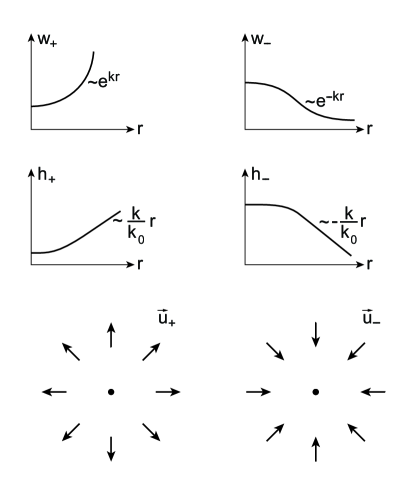
Figure 10: We show the two static radial modes for the Cole-Hopf, KPZ, and Burgers fields. The KPZ fields correspond to cones at large distance and paraboloids at short distances; the Burgers fields are outward-pointing and inward-pointing vector fields vanishing linearly at the origin.

Following Finkelstein Finkelstein et al. (1951) we finally give a simple argument based on dynamical system theory for the existence a radially symmetric bound states of the NLSE (84). Treating $r$ as a time variable Eq. (84) describes the motion of a particle of unit mass with $w$ as position in the double well potential $V(w)=-(k^{2}/2)w^{2}+(k_{0}^{2}/4)w^{4}$, subject to the time-dependent damping $(d-1)(dw/dr)/r$. The phase space is spanned by $w$ and $dw/dr$ and characterized by a saddle point at $(w,dw/dr)=(0,0)$ and an elliptic point at $(w,dw/dr)=(k/k_{0},0)$. The invariant homoclinic orbit (the separatrix) intersect the $w$ axis at $w=0$ and $w=\sqrt{2}k/k_{0}$. In Fig. 11 we have in a phase space plot depicted the constant energy surfaces $E=(1/2)(dw/dr)^{2}+V(w)$ in the absence of damping.

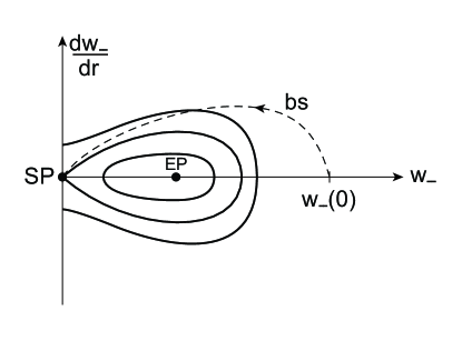
Figure 11: Phase space plot of $dw_{-}/dr$ vs. $w_{-}$. We depict the constant energy surfaces $E=(1/2)(dw/dr)^{2}+V(w)=\text{cst.}$ The dashed line corresponds to the radial bound state solution of the NLSE.

In $d=1$ the damping is absent and the bound state solution $w_{-}(x)\propto\cosh^{-1}kx$ corresponds to the motion along the invariant curve, the separatrix, from $w=\sqrt{2}k/k_{0}$ to the saddle point. For higher $d$, in the presence of damping, it follows from the equation of motion that $dE/dr=-(d-1)(dw/dr)^{2}/r<0$, i.e., the energy decreases monotonically in time. The orbit from an initial $w_{-}(0)$ with $dw_{-}/dr|_{r=0}=0$ will intersect the energy surfaces and in most cases spiral into the elliptic fixed point at $(k/k_{0},0)$. Only a particular orbit, corresponding to the bound state, will reach the saddle point at $(0,0)$ for $r\rightarrow\infty$. It follows from the numerical analysis that for increasing dimension, i.e., increasing damping, the initial value $w_{-}(0)$ defining the bound state solution migrates to larger values and out to infinity for $d\geq 4$. We have unsuccessfully attempted to determine the critical dimension by a dynamical system theory argument; however, in Sec. VIII we determine the upper critical dimension algebraically by means of an application of Derrick’s theorem.

V.3.2 Dynamical growth modes

The fundamental building blocks in establishing the growth morphology of the KPZ equation are the static localized modes $w_{\pm}^{0}(r)$, yielding the height fields $h_{\pm}^{0}(r)=(1/k_{0})\log w_{\pm}^{0}(r)$ and slope fields ${\bf u}_{\pm}^{0}=(1/k_{0}){\bm{\nabla}}w_{\pm}(r)/w_{\pm}^{0}(r)$. The growing mode $w_{+}^{0}$ is associated with the noiseless manifold $p=0$ and carries according to Eqs. (41), (45), and (49) no dynamics, i.e., $S^{\text{CH}}=H^{\text{CH}}=\Pi^{\text{CH}}=0$. The decaying bound state mode $w_{-}^{0}$, on the other hand, is endowed with dynamical attributes. The mode lives on the noisy manifold $p=\nu w$ and is associated with the noise field $p_{-}^{0}=\nu w_{-}^{0}$. According to Eqs. (45), (48), and (49) it carries action, energy, and momentum,

$$S^{\text{CH}}=\frac{1}{2}(k_{0}\nu)^{2}\int d^{d}xdt~{}w_{-}^{0}(r)^{4},$$ (90)

$$H^{\text{CH}}=-\frac{1}{2}(k_{0}\nu)^{2}\int d^{d}x~{}w_{-}^{0}(r)^{4},$$ (91)

$${\bm{\Pi}}^{\text{CH}}=0.$$ (92)

In order to generate dynamical modes we boost the static modes $w_{\pm}^{0}$ by means of the Galilei transformations (10), (11), (15), and (16). For the propagating localized Cole-Hopf, KPZ, and Burgers modes we then obtain

$$w_{\pm}({\bf r},t)=w_{\pm}^{0}(|{\bf r}+\lambda{\bf u}^{0}t|)\exp(k_{0}{\bf u}^{0}\cdot{\bf r}),$$ (93)

$$h_{\pm}({\bf r},t)=h_{\pm}^{0}(|{\bf r}+\lambda{\bf u}^{0}t|)+{\bf u}^{0}\cdot{\bf r},$$ (94)

$${\bf u}_{\pm}({\bf r},t)={\bf u}_{\pm}^{0}(|{\bf r}+\lambda{\bf u}^{0}t|)+{\bf u}^{0}.$$ (95)

The height field is a tilted d-dimensional cone moving with velocity $-\lambda{\bf u}^{0}$; the slope field a d-dimensional hedgehog structure with an imposed constant drift ${\bf u}^{0}$ moving with velocity $-\lambda{\bf u}^{0}$. In Fig. 12 we have shown the height and slope fields in 2D.

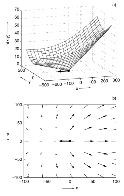
Figure 12: We depict the propagating height field and slope field modes in 2D. The bold arrows indicate the propagation velocity (arbitrary units).

Note that in 1D we have $w^{0}_{\pm}(x)\propto\cosh^{\pm}kx$, yielding $h^{0}_{\pm}(x)=(1/k_{0})\log|\cosh^{\pm}kx|+\text{cst.}$ and ${\bf u}^{0}_{\pm}(x)=\pm(k/k_{0})\tanh kx$, and we obtain the propagating modes $u_{\pm}(x,t)=\pm(k/k_{0})\tanh k(x+\lambda u^{0}t)+u^{0}$ discussed in Refs. Fogedby (1998b, 2003a)

The dynamics of the propagating modes is easily inferred. The noiseless mode $(w_{+},h_{+},{\bf u}_{+})$ on the $p=0$ manifold has vanishing action, energy, and momentum. The noisy mode $(w_{-},h_{-},{\bf u}_{-})$ on the $p_{-}=\nu w_{-}$ manifold carries finite action, energy, and momentum. Since the action is invariant under the the Galilean boost the action is given by Eq. (90). For the energy and momentum we obtain by insertion in Eqs. (41) and (49), noting that the noise field is transformed according to Eq. (50),

$$H^{\text{CH}}= -\frac{1}{2}(k_{0}\nu)^{2}\int d^{d}x~{}w_{-}^{0}(r)^{4}$$ (96)

$$+(k_{0}\nu)^{2}{\bf u}_{0}^{2}\int d^{d}x~{}w_{-}^{0}(r)^{2},~{}~{}~{}~{}~{}~{}~{}~{}~{}$$

$${\bm{\Pi}}^{\text{CH}}= -k_{0}\nu{\bf u}_{0}\int d^{d}x~{}w_{-}^{0}(r)^{2}.$$ (97)

Since the velocity of the $w_{-}$ mode is ${\bf v}=-\lambda{\bf u}^{0}$ the expressions (96) and (97) admit a particle interpretation. Defining the mass

$$m_{-}=\frac{1}{2}\int d^{d}xw_{-}^{0}(r)^{2},$$ (98)

we obtain

$${\bm{\Pi}}^{\text{CH}}=m_{-}{\bf v},$$ (99)

$$H^{\text{CH}}=E_{0}^{\text{CH}}+(1/2)m_{-}v^{2},$$ (100)

where

$$E_{0}^{\text{CH}}=-(1/2)(k_{0}\nu)^{2}\int d^{d}x~{}w_{-}^{0}(r)^{4}$$ (101)

is the rest energy.

VI Pattern Formation

The existence of the localized propagating growth modes in the Cole-Hopf field and the corresponding configurations in terms of the height and slope fields makes it natural to describe a growing interface in terms of a gas of growth modes. The implementation of this scheme constitutes a generalization of the weak noise approach in the 1D Burgers case to higher dimensions.

VI.1 General properties

From the general discussion in Sec. III and Sec. IV it follows that a solution of the Cole-Hopf field equations (43) and (44) from an initial configuration $w_{\text{i}}({\bf r})$ at time $t=0$ to a final configuration $w({\bf r})$ at time $T$, with the noise field $p({\bf r},t)$ as slaved variable, corresponds to a specific kinetic pathway, yielding according to Eqs. (45) and (46) the corresponding Arrhenius factor. The first central issue is thus to determine a global solution of the field equations. In the spirit of instanton calculations in field theory Coleman (1977); Das (1993); Rajaraman (1987) and following the scheme implemented in the case of the noisy 1D Ginzburg-Landau equation Fogedby (2005) and the noisy 1D Burgers equation Fogedby et al. (2004) we attempt to build a global solution on the basis of the propagating localized growth modes. In order to minimize overlap contributions we, moreover, consider the case of a dilute gas of growth modes. In order to characterize a kinetic pathway or growing interface we must, moreover, choose appropriate boundary conditions. Here it is natural to assume a flat interface at infinity, that is a vanishing slope field. Note that this boundary condition does not preclude an offset in the height field and thus allows for a propagation of facets or textures accounting for the nonequilibrium growth.

VI.2 Dynamical pair mode

In order to illustrate how to construct solutions we here consider a pair mode built from two growth modes. At time $t=0$ we combine a static noiseless and a static noisy Cole-Hopf mode centered at ${\bf r}_{1}$ and ${\bf r}_{2}$, respectively, and obtain the three equivalent pair fields:

$$w_{\text{pair}}({\bf r},0)=w_{+}^{0}({\bf r}-{\bf r}_{1})w_{-}^{0}({\bf r}-{\bf r}_{2}),$$ (102)

$$h_{\text{pair}}({\bf r},0)=h_{+}^{0}({\bf r}-{\bf r}_{1})+h_{-}^{0}({\bf r}-{\bf r}_{2}),$$ (103)

$${\bf u}_{\text{pair}}({\bf r},0)={\bf u}_{+}^{0}({\bf r}-{\bf r}_{1})+{\bf u}_{-}^{0}({\bf r}-{\bf r}_{2}).$$ (104)

For $r\rightarrow\infty$ we have ${\bf u}_{+}^{0}\sim(k_{1}/k_{0}){\bf r}/r$ and ${\bf u}_{-}^{0}\sim-(k_{2}/k_{0}){\bf r}/r$, where $k_{1}$ and $k_{2}$ are the inverse wavenumbers associated with the modes. Since ${\bf u}_{\text{pair}}({\bf r},0)\sim((k_{1}-k_{2})/k_{0}){\bf r}/r$ we ensure a vanishing slope field at infinity by balancing $k_{1}$ and $k_{2}$, i.e., $k_{1}=k_{2}=k$.

In order to assign velocities to the modes we note that in the vicinity of the mode position ${\bf r}_{1}$ the slope field is shifted by ${\bf u}_{-}^{0}({\bf r}_{1}-{\bf r}_{2})$ and we must, according to the Galilei transformation (15), assign the velocity ${\bf v}_{1}=-\lambda{\bf u}_{-}^{0}({\bf r}_{1}-{\bf r}_{2})$. Likewise, the mode ${\bf u}_{-}^{0}$ is assigned velocity ${\bf v}_{2}=-\lambda{\bf u}_{+}^{0}({\bf r}_{2}-{\bf r}_{1})$. For large separation $|{\bf r}_{1}-{\bf r}_{2}|\gg k^{-1}$ the asymptotic expressions (81) and (87) yield ${\bf v}_{1}=\lambda(k/k_{0})({\bf r}_{1}-{\bf r}_{2})/|{\bf r}_{1}-{\bf r}_{2}|$ and ${\bf v}_{2}=-\lambda(k/k_{0})({\bf r}_{2}-{\bf r}_{1})/|{\bf r}_{2}-{\bf r}_{1}|$. We note that ${\bf v}_{1}={\bf v}_{2}={\bf v}$, i.e., the individual modes propagate collectively in a direction along the axis ${\bf r}_{1}-{\bf r}_{2}$ of the pair mode. The propagating pair mode is thus given by

$$w_{\text{pair}}({\bf r},t)=w_{+}^{0}({\bf r}-{\bf v}t-{\bf r}_{1})w_{-}^{0}({\bf r}-{\bf v}t-{\bf r}_{2}),~{}~{}~{}~{}~{}~{}~{}~{}$$ (105)

$$h_{\text{pair}}({\bf r},t)=h_{+}^{0}({\bf r}-{\bf v}t-{\bf r}_{1})+h_{-}^{0}({\bf r}-{\bf v}t-{\bf r}_{2}),$$ (106)

$${\bf u}_{\text{pair}}({\bf r},t)={\bf u}_{+}^{0}({\bf r}-{\bf v}t-{\bf r}_{1})+{\bf u}_{-}^{0}({\bf r}-{\bf v}t-{\bf r}_{2}),$$ (107)

$${\bf v}=-\lambda{\bf u}_{+}^{0}({\bf r}_{2}-{\bf r}_{1}).$$ (108)

For the purpose of our discussion and assuming a dilute gas of growth modes it suffices to use the asymptotic forms of the Cole-Hopf, KPZ, and Burgers fields. Introducing a core radius $\epsilon$ of order $1/k$ in order to regularize the solution at the origin and introducing the notation

$$|{\bf r}|_{\epsilon}=\sqrt{{\bf r}^{2}+\epsilon^{2}},$$ (109)

we have for the propagating pair mode fields in more detail

$$w_{\text{pair}}({\bf r},t)\sim\exp(k|{\bf r}-{\bf r}_{1}(t)|_{\epsilon}-k|{\bf r}-{\bf r}_{2}(t)|_{\epsilon}),~{}~{}~{}~{}~{}~{}$$ (110)

$$h_{\text{pair}}({\bf r},t)\sim\frac{k}{k_{0}}(|{\bf r}-{\bf r}_{1}(t)|_{\epsilon}-|{\bf r}-{\bf r}_{2}(t)|_{\epsilon}),$$ (111)

$${\bf u}_{\text{pair}}({\bf r},t)\sim\frac{k}{k_{0}}\left(\frac{{\bf r}-{\bf r}_{1}(t)}{|{\bf r}-{\bf r}_{1}(t)|_{\epsilon}}-\frac{{\bf r}-{\bf r}_{2}(t)}{|{\bf r}-{\bf r}_{2}(t)|_{\epsilon}}\right),~{}~{}$$ (112)

$${\bf v}=-\lambda\frac{k}{k_{0}}\frac{{\bf r}_{2}-{\bf r}_{1}}{|{\bf r}_{2}-{\bf r}_{1}|_{\epsilon}},$$ (113)

$${\bf r}_{1,2}(t)={\bf v}t+{\bf r}_{1,2}.$$ (114)

Denoting the separation ${\bf d}={\bf r}_{2}-{\bf r}_{1}$ and the unit vector $\hat{\bf r}={\bf r}/r$, and expanding $h$ and ${\bf u}$ for large $r$ we obtain

$$h_{\text{pair}}({\bf r})=\frac{k}{k_{0}}\hat{\bf r}\cdot{\bf d},$$ (115)

$${\bf u}_{\text{pair}}({\bf r})={\frac{k}{k_{0}}\frac{1}{r}[{\bf d}-\hat{\bf r}}(\hat{\bf r}\cdot{\bf d})].$$ (116)

We note that the height field is constant at infinity, its value depending on the direction, whereas the slope field vanishes. Introducing polar coordinates where $\phi$ is the polar angle between the direction $\hat{\bf r}$ and the axis ${\bf d}$ we have

$$h_{\text{pair}}({\bf r})=\frac{k}{k_{0}}d\cos\phi,$$ (117)

$${\bf u}_{\text{pair}}({\bf r})=\frac{k}{k_{0}}\frac{1}{r}[{\bf d}-\hat{\bf r}d\cos\phi].$$ (118)

In 1D we obtain $w_{\pm}^{0}(x)\propto\cosh^{\pm 1}kx$, $h_{\pm}^{0}(x)\propto\pm(1/k_{0})\log|\cosh kx|$, $u_{\pm}^{0}(x)=\pm(k/k_{0})\tanh kx$, and $v=-\lambda(k/k_{0})$ and we have for the pair mode the expression

$$u(x,t)=$$

$$\frac{k}{k_{0}}[\tanh k(x-x_{1}(t))-\tanh k(x-x_{2}(t))],~{}~{}~{}~{}~{}~{}~{}$$ (119)

$$v=-\lambda\frac{k}{k_{0}},$$ (120)

$$x_{1,2}(t)=vt+x_{1,2},$$ (121)

in accordance with Eq. (107) and the discussion in Refs. Fogedby (2003a); the 1D pair mode is depicted in Fig. 6. In Fig. 13 we have depicted the height and slope fields in 2D.

Figure 13: We show the height and slope field of a dipole or pair mode in 2D. The bold arrows indicate the propagation velocity (arbitrary units).

The propagation of the pair mode is in the direction of the axis connecting the two centers ${\bf r}_{1}$ and ${\bf r}_{1}$. During the passage of a pair with velocity $v=\lambda k/k_{0}$ it follows from Eqs. (117) and (118) that the local height and slope fields change by $\delta h=2kd/k_{0}$ and $\delta u=2k/k_{0}$, respectively. The passage time of the pair is $\delta t=d/v=dk_{0}/\lambda k$ and we obtain for the growth velocity $\delta h/\delta t=2\lambda(k/k_{0})^{2}=(\lambda/2)(\delta u)^{2}$, in accordance with the averaged KPZ equation in a stationary state, $\langle\delta h/\delta t\rangle=(\lambda/2){\bf u}^{2}$.

The dynamics of the pair mode is inferred from Eqs. (90), (96), and (97). Inserting Eq. (89) a scaling argument yields

$$S_{\text{pair}}^{\text{CH}}=\frac{1}{2}(k_{0}\nu)^{2}T\left(\frac{k}{k_{0}}\right)^{4}a_{d}^{4}k^{-d}\int_{0}^{\infty}d^{d}\xi~{}f(\xi)^{4},$$ (122)

for the action of a pair propagating in time $T$. Note that only the decaying bound state component carries action. In the dynamical phase space language this scenario corresponds to a pair-orbit from an initial configuration $w_{\text{i}}({\bf r},0)=w_{+}^{0}({\bf r}-{\bf r}_{1})w_{-}^{0}({\bf r}-{\bf r}_{2})$ with initial noise field $p_{\text{i}}({\bf r},0)=\nu w_{-}^{0}({\bf r}-{\bf r}_{2})$ to a final configuration $w_{\text{f}}({\bf r},T)=w_{+}^{0}({\bf r}-{\bf v}T-{\bf r}_{1})w_{-}^{0}({\bf r}-{\bf v}T-{\bf r}_{2})$ and $p_{\text{f}}({\bf r},T)=\nu w_{-}^{0}({\bf r}-{\bf v}T-{\bf r}_{2})$. In Fig. 14 we have in a $(w,p)$ phase space plot sketched the specific orbit from $(w_{\text{i}},p_{\text{i}})$ to $(w_{\text{f}},p_{\text{f}})$.

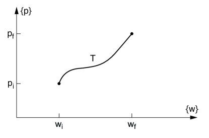
Figure 14: Phase space plot of a dipole or pair orbit from an initial configuration $w_{\text{i}}$ to a final configuration $w_{\text{f}}$ in transition time $T$. The noise field $p$ is a slaved variable going from $p_{\text{i}}$ to $p_{\text{f}}$.

Choosing the centers ${\bf r}_{1}$ and ${\bf r}_{2}$ and the amplitude $k$ we thus have a whole class of orbits corresponding to kinetic transitions from $({\bf r}_{1},{\bf r}_{2},k)$ at time $t=0$ to $({\bf r}_{1}+{\bf v}T,{\bf r}_{2}+{\bf v}T,k)$ at time $T$; note that the magnitude of the velocity is $v=\lambda k/k_{0}$, whereas its direction is given by ${\bf d}={\bf r}_{1}-{\bf r}_{2}$.

For the rest energy and mass of the pair mode we have, inserting Eq. (89) in Eqs. (96), (97), (98), and (101),

$$E_{0,\text{pair}}=-\frac{1}{2}(k_{0}\nu)^{2}T\left(\frac{k}{k_{0}}\right)^{4}a_{d}^{4}k^{-d}\int d^{d}\xi~{}f(\xi)^{4},~{}~{}~{}~{}~{}~{}~{}$$ (123)

$$m_{\text{pair}}=\frac{1}{2}\left(\frac{k}{k_{0}}\right)^{2}a_{d}^{2}k^{-d}\int d^{d}\xi~{}f(\xi)^{2},$$ (124)

and we obtain  for the energy and momentum

$$E_{\text{pair}}=E_{0,\text{pair}}+\frac{1}{2}m_{\text{pair}}{\bf v}^{2},$$ (125)

$${\bm{\Pi}}_{\text{pair}}=m_{\text{pair}}{\bf v},$$ (126)

$${\bf v}=-\lambda\frac{k}{k_{0}}{\bf d}.$$ (127)

The pair mode satisfying the boundary conditions of an asymptotically flat interface suggests an independent particle picture of the growth morphology in terms of a dilute gas of pair modes. The pair modes have masses scaling with the amplitude according to $m_{\text{pair}}\propto k^{2-d}$. In 2D the mass is independent of $k$, in 1D the mass grows linearly with $k$, for $d>2$ the mass vanishes for large $k$. The rest energy $E_{0,\text{pair}}\propto k^{4-d}$, i.e., $E_{0,\text{pair}}$ is independent of $k$ for $d=4$. For $d<4$, $E_{0,\text{pair}}$ grows with $k$, for $d>4$, $E_{0,\text{pair}}$ vanishes for large $k$. Finally, the velocity scales linearly with $k$.

VI.3 Dynamical network

The generalization to a network of propagating modes is straightforward. At time $t=0$ we assign a set of growing and decaying static modes at the positions ${\bf r}_{i}^{0}$, $i=1,\cdots$, and obtain the Cole-Hopf field at time $t=0$,

$$w({\bf r},0)=\prod_{i}w_{i}^{0}({\bf r}-{\bf r}_{i}^{0}).$$ (128)

It is here convenient to use a charge language for the amplitudes $k_{i}$ pertaining to the $i$-th mode. For $k_{i}>0$, a positive charge, $w_{i}^{0}({\bf r})$ is a growing solution of the linear equation (77); for $k_{i}<0$, a negative charge, $w_{i}^{0}({\bf r})$ is a decaying bound state solution of the NLSE (83). For large $r$ we have $w_{i}^{0}({\bf r}-{\bf r}_{i}^{0})\sim\exp(k_{i}r)$, i.e., $w({\bf r},0)\sim\exp(r\sum_{i}k_{i})$ and in order to ensure an asymptotically flat interface $h({\bf r})=(1/k_{0})\log w({\bf r})$ we impose the charge neutrality condition

$$\sum_{i}k_{i}=0.$$ (129)

The corresponding initial height and slope field are then given by

$$h({\bf r},0)=\frac{1}{k_{0}}\sum_{i}\log w_{i}^{0}({\bf r}-{\bf r}_{i}^{0}),$$ (130)

$${\bf u}({\bf r},0)=\frac{1}{k_{0}}\sum_{i}\frac{{\bm{\nabla}}w_{i}^{0}({\bf r}-{\bf r}_{i}^{0})}{w_{i}^{0}({\bf r}-{\bf r}_{i}^{0})}.$$ (131)

In order to assign velocities to the modes we proceed as in the case of the pair mode. At the position ${\bf r}^{0}_{\ell}$ of the $\ell$-th mode the slope field is shifted by ${\bf u}({\bf r}_{\ell}^{0},0)=(1/k_{0})\sum_{i}{\bm{\nabla}}w_{i}^{0}({\bf r}_{\ell}^{0}-{\bf r}_{i}^{0})/w_{i}^{0}({\bf r}_{\ell}^{0}-{\bf r}_{i}^{0})$, corresponding to a Galilei boost to velocity ${\bf v}_{\ell}=\lambda{\bf u}({\bf r}_{\ell}^{0},0)$. Since, unlike the case of a pair, the modes move relative to one another the network will converge towards a self consistent state. We thus obtain the self consistent dynamical network

$$w({\bf r},t)=\prod_{i}w_{i}^{0}({\bf r}-{\bf r}_{i}(t)),$$ (132)

$${\bf r}_{i}(t)=\int_{0}^{t}{\bf v}_{i}(t^{\prime})dt^{\prime}+{\bf r}_{i}^{0},$$ (133)

$${\bf v}_{i}(t)=-2\nu\sum_{\ell\neq i}\frac{{\bm{\nabla}}w_{i}^{0}({\bf r}_{i}(t)-{\bf r}_{\ell}(t))}{w_{i}^{0}({\bf r}_{i}(t)-{\bf r}_{\ell}(t))},$$ (134)

$$\sum_{i}k_{i}=0.$$ (135)

The interpretation of the growth morphology or pattern formation represented by Eq. (132-135) is straightforward. In the weak noise WKB representation the growing interface is described by a gas of growth modes with negative and positive charges. The asymptotic flatness condition is ensured by imposing charge neutrality as expressed by Eq. (135). The dynamics of the network is constrained by the assignment of velocities to the modes, where according to Eq. (134) the velocity of a particular mode depends on the position and charges of the other modes. The connectivity and continuity of the network thus defines the temporal evolution.

For the present purposes it is sufficient to consider a dilute network and use the asymptotic form $w_{i}^{0}({\bf r})\sim\exp(k_{i}r)$. We then obtain the height field, slope field, and assigned velocities

$$h({\bf r},t)=\frac{1}{k_{0}}\sum_{i}k_{i}|{\bf r}-{\bf r}_{i}(t)|_{\epsilon},$$ (136)

$${\bf u}({\bf r},t)=\frac{1}{k_{0}}\sum_{i}k_{i}\frac{{\bf r}-{\bf r}_{i}(t)}{|{\bf r}-{\bf r}_{i}(t)|_{\epsilon}},$$ (137)

$${\bf v}_{i}(t)=-2\nu\sum_{\ell\neq i}k_{\ell}\frac{{\bf r}_{i}(t)-{\bf r}_{\ell}(t)}{|{\bf r}_{i}(t)-{\bf r}_{\ell}(t)|_{\epsilon}},$$ (138)

where we have used the short distance or UV regularization given by Eq. (109).

Since we initialize the network at rest, it will pass thorough a transient period where the velocities adjust to constant values as the modes recedes from one another. From Eq. (138) we obtain by differentiation $d{\bf v}_{i}/dt=-2\nu\sum_{\ell\neq i}[({\bf v}_{i}-{\bf v}_{\ell})/|{\bf r}_{i}-{\bf r}_{\ell}|_{\epsilon}-({\bf r}_{i}-{\bf r}_{\ell})\cdot({\bf v}_{i}-{\bf v}_{\ell})({\bf r}_{i}-{\bf r}_{\ell})/|{\bf r}_{i}-{\bf r}_{\ell}|_{\epsilon}^{3}]$ which, assuming ${\bf v}_{i}-{\bf v}_{\ell}$ to be bounded, vanishes for $|{\bf r}_{i}-{\bf r}_{\ell}|\rightarrow\infty$. We infer that at intermediate times longer than the transient time the velocities attain constant values. Using ${\bf r}_{i}(t)={\bf v}_{i}t+{\bf r}_{i}^{0}$ we thus obtain from Eq. (138) a self consistent equation for the velocities in the stationary state

$${\bf v}_{i}=-2\nu\sum_{\ell\neq i}k_{\ell}\frac{{\bf v}_{i}-{\bf v}_{\ell}}{|{\bf v}_{i}-{\bf v}_{\ell}|_{\epsilon}}.$$ (139)

At fixed time for ${\bf r}$ large expanding Eq. (136) we obtain

$$h({\bf r},t)\sim-\frac{1}{k_{0}}\frac{{\bf r}}{r}\sum_{i}k_{i}{\bf r}_{i}(t),$$ (140)

where we have used the neutrality condition (135), i.e., an asymptotically flat interface. $\sum_{i}k_{i}{\bf r}_{i}(t)$ defines a center of mass position ${\bf R}(t)=\sum_{i}k_{i}{\bf r}_{i}(t)$ for a dilute cluster of modes. Introducing the polar angle $\phi$ between the direction ${\bf r}/r$ and ${\bf R}(t)$ we have, in analogy to Eqs. (117) and (118) in the case of the pair mode, $h({\bf r},t)=-(1/k_{0})|{\bf R}(t)|\cos\phi$, and the height offset depends on the direction. As the cluster of modes propagate across the system the height field changes by $2|{\bf R}(t)|/k_{0}$. Likewise, for the slope field ${\bf u}$ expanding Eq. (137) for large ${\bf r}$ we have ${\bf u}({\bf r},t)\sim({\bf r}/r)\sum_{i}k_{i}=0$, i.e., asymptotically a flat interface. We also note that ${\bf R}(t)=\sum_{i}k_{i}({\bf r}_{i}^{0}+{\bf v}_{i}t)=\sum_{i}k_{i}({\bf r}_{i}^{0}+{\bf v}_{i}t)=\sum_{i}k_{i}{\bf r}_{i}^{0}$, where we have used $\sum_{i}k_{i}{\bf v}_{i}=0$, following from Eq. (139), i.e., ${\bf R}(t)=\sum_{i}k_{i}{\bf r}_{i}^{0}$ is independent of time in the stationary state. Likewise, at fixed position for $t$ large we have by expanding Eq. (136), $h({\bf r},t)=(t/k_{0})\sum_{i}k_{i}v_{i}$, and we infer the constant growth velocity

$$v=\frac{dh}{dt}=\frac{1}{k_{0}}\sum_{i}k_{i}v_{i}.$$ (141)

The relationship between the imposed drift $F$ in the KPZ equation (1) and the charge assignment to the growth modes, $\{k_{i}\}$, is given by

$$F=\frac{2\nu^{2}}{\lambda}\left(\sum_{i}k_{i}\right)^{2}.$$ (142)

In order to demonstrate this identity we consider the Cole-Hopf field equation (60) in the asymptotic regions where the noise field vanishes, $\partial w/\partial t=\nu{\bm{\nabla}}^{2}w-\nu k^{2}w$, $k^{2}=\lambda F/2\nu^{2}$. From the growth mode ansatz $w=\prod_{i}\exp k_{i}|{\bf r}-{\bf r}_{i}(t)|$ we readily obtain $(\partial w/\partial t)/w=-\sum_{i}k_{i}{\bf v}_{i}\cdot({\bf r}-{\bf r}_{i}(t))/|{\bf r}-{\bf r}_{i}(t)|$ and ${\bm{\nabla}}^{2}w/w=\sum_{ij}k_{i}k_{j}({\bf r}-{\bf r}_{i}(t))\cdot({\bf r}-{\bf r}_{j}(t))/|{\bf r}-{\bf r}_{i}(t)||{\bf r}-{\bf r}_{j}(t)|$. Inserting the mode velocity from Eq. (138) and symmetrizing we have for large ${\bf r}$ the identity (142). The drift $F$ is thus given by the total charge of the growth modes. A neutral system with vanishing slope at infinity corresponds to $F=0$.

In addition to the dynamical velocity constraint imposed by the continuity and connectivity of the network, the canonical structure of the WKB weak noise scheme impart dynamical attributes to the network. As far as the dynamics is concerned only modes with negative charge on the noise manifolds $p_{i}=\nu w_{i}$, corresponding to the bound state solution of the NLSE, contribute. According to Eq. (90) we obtain for the total action of the network

$$S_{\text{net}}=\sum_{k_{i}<0}S_{i},$$ (143)

where the action of the i-th mode is

$$S_{i}=\frac{1}{2}(k_{0}\nu)^{2}T\int d^{d}x~{}w_{i}^{0}(r)^{4}.$$ (144)

For a dilute network using the asymptotic expression (122) we obtain accordingly

$$S_{i}=\frac{1}{2}(k_{0}\nu)^{2}T\left(\frac{k_{i}}{k_{0}}\right)^{4}a_{d}^{4}k^{-d}\int_{0}^{\infty}d^{d}\xi~{}f(\xi)^{4}.$$ (145)

At time $t=0$ we assign an initial state $w_{i}({\bf r},0)$ by choosing a set of positions ${\bf r}_{i}^{0}$ and associated charges $k_{i}$. The expressions (138) and (133) subsequently determine the appropriate propagation velocities and time dependent positions. The network develops dynamically defining a particular kinetic pathway. In order to obtain a specific path from an initial state $w_{\text{i}}$ to a final state $w_{\text{f}}$ traversed in time $T$ we must choose a specific set of positions and charges. The action associated with the path is then given by Eqs. (143-145), yielding the Arrhenius factor $P\propto\exp[-S/\Delta]$ for the corresponding transition probability.

Associated with the initial configuration $w_{\text{i}}$ at time $t=0$ is the initial noise field

$$p_{\text{i}}({\bf r},0)\propto\prod_{k_{i}<0}w_{i}^{0}({\bf r}-{\bf r}_{i}^{0}).$$ (146)

Assigning velocities the noise field propagates according to

$$p({\bf r},t)\propto\prod_{k_{i}<0}w_{i}^{0}({\bf r}-{\bf v}_{i}t-{\bf r}_{i}^{0}),$$ (147)

to the final noise configuration at time $T$. For a fixed transition time $T$ and a given initial $w$-configuration different assignments of $k_{i}$ and ${\bf r}_{i}^{0}$ yield different noise field and, correspondingly, different final $(w,p)$ configurations. The scenario is depicted schematically in Fig. 15

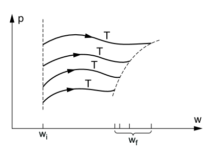
Figure 15: Phase space plot of a set of orbits with the same transition time $T$ terminating in different final configurations $w_{\text{f}}$.

The energy and momentum of a network is inferred from Eqs. (123-127)

$$E_{\text{net}}=E_{\text{net},0}+\frac{1}{2}\sum_{i}m_{i}v_{i}^{2},$$ (148)

$$E_{\text{net},0}=$$

$$-\frac{1}{2}(k_{0}\nu)^{2}\sum_{k_{i}<0}\left(\frac{k_{i}}{k_{0}}\right)^{4}a_{d}^{4}k_{i}^{-d}\int d^{d}\xi~{}f(\xi)^{4},~{}~{}~{}~{}~{}~{}~{}$$ (149)

$$m_{i}=\frac{1}{2}\left(\frac{k_{i}}{k_{0}}\right)^{2}a_{d}^{2}k_{i}^{-d}\int d^{d}\xi~{}f(\xi)^{2},$$ (150)

$${\bm{\Pi}}_{\text{net}}=\sum_{k_{i}<0}m_{i}{\bf v}_{i},$$ (151)

where in the stationary state ${\bf v}_{i}$ is given by Eq. (139).

VI.4 Field theory

In a qualitative sense the Cole-Hopf field $w$ and the associated noise field $p$ governed by Eqs. (43) and (44) representing the KPZ equation in the weak noise limit plays the role of bare fields, whereas the propagating noiseless and noisy modes $w_{i}^{0}$ together with the associated noise fields connected in a dynamical network constitute the renormalized fields. The strong coupling features of the problem are thus represented by the network. It is instructive to represent this insight in terms of a field theory for the network. Below we sketch aspects of such a field theory.

We consider a dilute distribution of modes or monopoles with charges $k_{i}$ at positions $r_{i}$ and introduce the density $n$ and charge density $\rho$ according to

$$n({\bf r},t)=\sum_{i}\delta^{d}({\bf r}-{\bf r}_{i}(t)),$$ (152)

$$\rho({\bf r},t)=\sum_{i}k_{i}\delta^{d}({\bf r}-{\bf r}_{i}(t));$$ (153)

we note that the neutrality condition $\sum_{i}k_{i}=0$ is equivalent to $\int d^{d}x\rho({\bf r},t)=0$. For the asymptotic height and slope fields (136) and (137) we obtain

$$h({\bf r},t)=\frac{1}{k_{0}}\int d^{d}x^{\prime}~{}\rho({\bf r}^{\prime},t)|{\bf r}-{\bf r}^{\prime}|_{\epsilon},$$ (154)

$${\bf u}({\bf r},t)=\frac{1}{k_{0}}\int d^{d}x^{\prime}~{}\rho({\bf r}^{\prime},t)\frac{{\bf r}-{\bf r}^{\prime}}{|{\bf r}-{\bf r}^{\prime}|_{\epsilon}}.$$ (155)

Introducing the velocity field

$${\bf v}({\bf r},t)=\sum_{i}{\bf v}_{i}(t)\delta^{d}({\bf r}-{\bf r}_{i}(t)),$$ (156)

we express the velocity condition (138) in the form

$${\bf v}({\bf r},t)=-2\nu n({\bf r},t){\bf u}({\bf r},t).$$ (157)

Using ${\bm{\nabla}}\cdot({\bf r}/r)=(d-1)/r$ and introducing the scalar field or potential $\phi$

$$\phi={\bm{\nabla}}\cdot{\bf u}=\nabla^{2}h,$$ (158)

we have from Eq. (156)

$$\phi({\bf r},t)=\frac{d-1}{k_{0}}\int d^{d}x^{\prime}~{}\frac{\rho({\bf r}^{\prime},t)}{|{\bf r}-{\bf r}^{\prime}|_{\epsilon}},$$ (159)

i.e., $\phi$ is analogous to the electric potential arising from a charge distribution $\rho({\bf r},t)$ Landau and Lifshitz (1960). It also follow from Eq (159) that $\phi$ satisfies the fractional Poisson equation

$$\nabla^{d-1}\propto\frac{d-1}{k_{0}}\rho,$$ (160)

where $\nabla^{d-1}$ is the Fourier transform of $k^{d-1}$; note that in $d=3$ Eq. (160) becomes the usual Poisson equation in electrostatics Landau and Lifshitz (1960).

The charge distribution $\rho$ yields the potential $\phi$ either as a solution of Eq. (160) or in terms of the integrated form in Eq. (159). Inserting Eq. (158) we also have

$$\nabla^{d+1}h\propto\frac{d-1}{k_{0}}\rho,$$ (161)

$$\nabla^{d-1}{\bm{\nabla}}\cdot{\bf u}\propto\frac{d-1}{k_{0}}\rho.$$ (162)

The equation of motion for the charges is given by Eq. (157) which determine the velocity field ${\bf v}$ in terms of the slope field ${\bf u}$. It is instructive to compare Eq. (156) to the Lorentz equation for the motion of charges $e$ with density $n$ in an electric field ${\bf E}$, $md{\bf v}/dt=en{\bf E}$. Including a damping term $-\gamma{\bf v}$ and considering the overdamped case we obtain ${\bf v}=-(e/\gamma)n{\bf E}$ which has the same form as Eq. (157) with the slope field playing the role of an electric field.

Finally, introducing the continuity equations expressing number and charge conservation

$$\frac{\partial n}{\partial t}+{\bm{\nabla}}\cdot{\bf v}=0,$$ (163)

$$\frac{\partial\rho}{\partial t}+{\bm{\nabla}}\cdot{\bf j}=0,$$ (164)

where the current density is

$${\bf j}({\bf r},t)=\sum_{i}k_{i}{\bf v}_{i}\delta^{d}({\bf r}-{\bf r}_{i}(t)),$$ (165)

we have the field equation (162) for ${\bf u}$ and the Lorentz equation (157) for the particle dynamics. In Fig. 16 we depict a neutral three-mode configuration in the height field and the associated divergence of the slope field. ${\bm{\nabla}}\cdot{\bf u}$ clearly shows the two negative charges and the single positive charge constituting the morphology.

Figure 16: We depict a neutral three-mode configuration in the height field and the associated divergence of the slope field (arbitrary units).

VI.5 Linear diffusive modes

Generalizing the discussion in the case of the 1D noisy Burgers equation to higher dimension, it is clear that in addition to the network of growth modes there are also superimposed linear diffusive modes. Here we summarize aspects of the linear mode spectrum.

VI.5.1 The linear case

In the linear Edwards-Wilkinson case the weak noise field equations (52) and (53) take the form

$$\frac{\partial{\bf u}}{\partial t}=\nu\nabla^{2}{\bf u}-{\bm{\nabla}}({\bm{\nabla}}\cdot{\bf p}),$$ (166)

$$\frac{\partial{\bf p}}{\partial t}=-\nu\nabla^{2}{\bf u}.$$ (167)

Since ${\bf u}(={\bm{\nabla}}h)$ is longitudinal and since only the longitudinal component of ${\bf p}$ couple to ${\bf u}$, Eqs. (166) and (167) for the wavenumber components ${\bf u}_{\bf k}$ and ${\bf p}_{\bf k}$ correspond to the overdamped oscillator case discussed in appendix A. For an orbit from ${\bf u}^{\text{i}}_{\bf k}$ at time $t=0$ to ${\bf u}^{\text{f}}_{\bf k}$ at $t=T$, with ${\bf p}_{\bf k}$ as slaved variable, we have

$${\bf u}_{\bf k}(t)=\frac{{\bf u}^{f}_{\bf k}\sinh\omega_{\bf k}t+{\bf u}^{i}_{\bf k}\sinh\omega_{\bf k}(T-t)}{\sinh\omega_{\bf k}T},$$ (168)

$${\bf p}_{\bf k}(t)=\nu e^{\omega_{\bf k}t}\frac{{\bf u}^{f}_{\bf k}-{\bf u}^{i}_{\bf k}e^{-\omega_{\bf k}T}}{\sinh\omega_{\bf k}T},$$ (169)

with the diffusive mode frequency

$$\omega_{\bf k}=\nu{\bf k}^{2}.$$ (170)

The spectrum is exhausted by linear diffusive modes with gapless dispersion given by Eq. (170). Following Ref. Fogedby (2003a) the action and transition probabilities are given by

$$S=\nu\int\frac{d^{d}k}{(2\pi)^{d}}~{}\frac{|{\bf u}_{\bf k}^{f}-{\bf u}^{i}_{\bf k}\exp(-\omega_{\bf k}T)|^{2}}{1-\exp(-2\omega_{\bf k}T)},$$ (171)

$$P({\bf u}_{\bf k}^{f},{\bf u}^{i}_{\bf k},T)\propto\exp\left[-\frac{S}{\Delta}\right].$$ (172)

In the limit $T\rightarrow\infty$ we obtain the stationary distribution

$$P_{0}({\bf u}_{\bf k})\propto\exp\left[-\frac{\nu}{\Delta}\int\frac{d^{d}k}{(2\pi)^{d}}~{}|{\bf u}_{\bf k}|^{2}\right],$$ (173)

yielding the Boltzmann distribution (5); for more comments on the linear case see the discussion in Sec. II.

VI.5.2 The nonlinear growth case

In the nonlinear KPZ case the growth morphology or pattern formation is given by a dynamical network of propagating localized growth modes. Superimposed on the dynamical network is a spectrum of extended linear diffusive modes. In order to implement the boundary condition of an asymptotically flat interface it is most convenient to conduct the discussion in terms of the slope field ${\bf u}$.

Considering the field equations (52) and (53) we set ${\bf u}={\bf u}_{\text{net}}+\delta{\bf u}$ and ${\bf p}={\bf p}_{\text{net}}+\delta{\bf p}$. Here ${\bf u}_{\text{net}}$ is given by (137), i.e.,

$${\bf u}_{\text{net}}({\bf r},t)=\frac{1}{k_{0}}\sum_{i}k_{i}\frac{{\bf r}-{\bf r}_{i}(t)}{|{\bf r}-{\bf r}_{i}(t)|_{\epsilon}}.$$ (174)

For the associated noise field ${\bf p}_{\text{net}}$ we obtain from Eqs. (65), (85), and (66) for a single mode $\tilde{p}=k_{0}pw=k_{0}\nu w_{-}^{2}\propto k_{0}\nu r^{1-d}\exp(-2kr)$, i.e., ${\bm{\nabla}}\cdot{\bf p}=-k_{0}\nu r^{1-d}\exp(-2kr)$. Setting ${\bf p}=({\bf r}/r)g(r)$ we have $dg/dr+((d-1)/r)g=-k_{0}\nu r^{1-d}\exp(-2kr)$ with asymptotic solution $g(r)\sim(k_{0}\nu/2k)r^{1-d}\exp(-2kr)$. Generalizing to a propagating network we have

$${\bf p}_{\text{net}}({\bf r},t)=\frac{\nu k_{0}}{2}\sum_{k_{i}<0}\frac{{\bf r}-{\bf r}_{i}(t)}{|k_{i}||{\bf r}-{\bf r}_{i}(t)|^{d}_{\epsilon}}e^{-2|k_{i}||{\bf r}-{\bf r}_{i}(t)|}.~{}~{}$$ (175)

We note that the noise field is localized in the vicinity of the modes with negative charge, i.e., the modes carrying dynamics. The noise field falls off exponentially with a range given by $|k_{i}|^{-1}$. Confining our discussion to the regions between the growth modes and noting that $p_{\text{net}}\sim 0$ and $\nabla{\bf u_{\text{net}}}\sim 0$ we obtain linear equations for $\delta{\bf u}$ and $\delta{\bf p}$,

$$\frac{\partial\delta{\bf u}}{\partial t}=\nu\nabla^{2}\delta{\bf u}+\lambda({\bf u}_{\text{net}}\cdot{\bm{\nabla}})\delta{\bf u}+{\bm{\nabla}}({\bm{\nabla}}\cdot\delta{\bf p}),~{}~{}~{}~{}$$ (176)

$$\frac{\partial\delta{\bf p}}{\partial t}=-\nu\nabla^{2}\delta{\bf p}+\lambda({\bf u}_{\text{net}}\cdot{\bm{\nabla}})\delta{\bf p}.$$ (177)

Assuming that ${\bf u}_{\text{net}}\sim\text{const.}$ and setting $\delta{\bf u},\delta{\bf p}\sim\exp(-Et)\exp(i{\bf k}{\bf r})$ it follows that

$$\delta{\bf u}=({\bf a}e^{-(\nu k^{2}-i\lambda{\bf u}_{\text{net}}\cdot{\bf k})t}+{\bf b}e^{(\nu k^{2}+i\lambda{\bf u}_{\text{net}}\cdot{\bf k})t})e^{i{\bf k}{\bf r}},~{}~{}~{}~{}~{}~{}~{}$$ (178)

$$\delta{\bf p}={\bf c}e^{(\nu k^{2}+i\lambda{\bf u}_{\text{net}}\cdot{\bf k})t}e^{i{\bf k}{\bf r}}.$$ (179)

For $\lambda=0$ we recover the linear case; in the nonlinear case, incorporating the time dependent term $i\lambda{\bf u}_{\text{net}}\cdot{\bf k}t$ in the plane wave phase $i{\bf k}{\bf r}$, we note that the diffusive modes undergoes a mode transmutation to damped and growing propagating modes with phase velocity $\lambda{\bf u}_{\text{net}}\cdot{\bf k}$.

VII Stochastic interpretation

The weak noise scheme gives access to the transition probability $P(h_{\text{i}}\rightarrow h_{\text{f}},T)$ from an initial height profile $h_{\text{i}}$ to a final profile $h_{\text{f}}$ in time $T$, where $P$ is given in terms of the action $S(h_{\text{i}}\rightarrow h_{\text{f}},T)$, $P\propto\exp[-S/\Delta]$. We note that the scheme only yields what corresponds to the Arrhenius factor $\exp[-S/\Delta]$; the prefactor $\Gamma(T)$, $P(T)=\Gamma(T)\exp[-S(T)/\Delta]$, is to leading order in $\Delta$ determined by the normalization condition $\int\prod_{\bf r}dh_{\text{f}}P(h_{\text{i}}\rightarrow h_{\text{f}},T)=1$, i.e., $\Gamma^{-1}(T)=\int\prod_{\bf r}dh_{\text{f}}P(h_{\text{i}}\rightarrow h_{\text{f}},T)$, see also Refs. Fogedby (2003a); Fogedby et al. (2004).

VII.1 Kinetic transitions

The prescription is in principle straightforward. An initial configuration $h_{\text{i}}$ at time $t=0$ is modelled or approximated by a dilute gas of growth modes forming the network characterized by their charges $\{k_{i}\}$ and positions $\{{\bf r}_{i}^{0}\}$ plus a spectrum of diffusive modes $\{\delta u_{k}^{\text{i}},\delta p_{k}^{\text{i}}\}$. The dynamical configuration evolves in time according to the field equations. The velocities of the growth modes are assigned according to Eqs. (134) and (138); notice that the noise field associated with the negatively charged modes develops in time according to Eq. (175). At time $t=T$ the profile $h$ has evolved to the final profile $h_{\text{f}}$, corresponding to the network configuration $\{k_{i},{\bf r}_{i}(T)\}$ and the final diffusive mode configuration $\{\delta u_{k}^{\text{f}},\delta p_{k}^{\text{f}}\}$. This time evolution corresponds to a specific kinetic pathway for a growing interface. The action associated with the transition is composed of a network part $S_{\text{net}}$ and a diffusive mode part $S_{\text{diff}}$. $S_{\text{net}}$ is given by Eqs. (143), (144), and (145) and thus only depends on $\{k_{i}\}$ for the negatively charged bound states or monopoles. In the linear case $S_{\text{diff}}$ is given by Eq. (171); we note that $S_{\text{diff}}$ depends on the initial and final diffusive mode amplitudes $\delta u_{k}^{\text{i}}$ and $\delta u_{k}^{\text{f}}$. At long times $S_{\text{net}}$ grows linearly with $T$, like in the case of random walk discussed in appendix A, whereas $S_{\text{diff}}$ approaches the stationary form $\nu\int d^{d}k/(2\pi)^{d}|{\bf u}_{k}^{\text{f}}|^{2}$, see Eq. (173), as in the case of the overdamped oscillator discussed in appendix A.

VII.2 Anomalous diffusion and scaling in the dipole sector

Leaving aside the issue of the linear diffusive modes, the network representation is based on an assumption of a dilute gas of growth modes or charged monopoles. In the course of time the modes will in general collide and coalesce and the dilute gas approximation ceases to be valid. Here we consider the class of network configurations composed of a dilute gas of pair modes or dipoles. A single dipole satisfies the boundary condition of vanishing slope field. Consequently, the dipoles move independently.

A single dipole or pair mode with charges $k$ and $-k$ propagate according to Eq. (127) with velocity

$$v=\lambda\frac{k}{k_{0}},$$ (180)

and carries according to Eq. (122) the action

$$S=Tk^{4-d}\left(\frac{\nu}{k_{0}}\right)^{2}A,$$ (181)

where $A=a_{d}^{4}\int_{0}^{\infty}d^{d}\xi~{}f(\xi)$ only depends on dimension. During time $T$ the center of mass of the dipole propagates the distance $L=vT$ and eliminating the charge $k$ we obtain the action

$$S=\frac{L^{4-d}}{T^{3-d}}B,$$ (182)

where $B=\lambda^{-2}\nu^{d}2^{d-2}A$.

The form of Eq. (182) allows an interpretation of the ballistic motion of the dipoles within the dynamical scheme as a random motion within the stochastic description. From the WKB ansatz we obtain for the transition probability $P(L,T)$ over a distance $L$ in time $T$ for a single dipole

$$P(L,T)\propto\exp\left[-\frac{B}{\Delta}\frac{L^{4-d}}{T^{3-d}}\right].$$ (183)

By a simple scaling argument the mean square displacement is given by

$$\langle\delta L^{2}\rangle=T^{2H}\left[\frac{\Delta}{B}\right]^{2(1-H)}\Gamma(3-2H),$$ (184)

where $\Gamma(z)$ is the Gamma function Lebedev (1972) and we have introduced the Hurst exponent Feder (1988)

$$H=\frac{3-d}{4-d}.$$ (185)

From the scaling form in Eq. (17) and from Eq. (183) it also follows that the dynamic exponent for the dipole sector is $z=1/H$, i.e.,

$$z=\frac{4-d}{3-d}.$$ (186)

In 1D we obtain $H=2/3$ and $z=3/2$ in accordance with well-established results for the KPZ equation or, equivalently, the noisy Burgers equation. Here the dynamic exponent for the dipole sector agrees with the exact value. Note that the scaling law (18), $z+\zeta=2$, following from Galilean invariance and automatically implemented in the present approach, implies the roughness exponent $\zeta=1/2$. The Hurst exponent $H=2/3>1/2$ corresponds to a persistent random walk. Since the mean square displacement for $H=2/3>1/2$ falls off faster than Brownian walk ($H=1/2$) we have the case of superdiffusion. In 2D, which in a scaling context is the lower critical dimension, we have $H=1/2$, corresponding to ordinary Brownian diffusion. The dynamic exponent $z=2$ and according to $z+\zeta=2$ the roughness exponent $\zeta=0$, corresponding to a smooth interface. In 3D the Hurst exponent $H=0$ corresponding to the logarithmic case

$$\langle\delta L^{2}\rangle\propto\log T~{}~{}\text{for}~{}~{}d=3.$$ (187)

Here the mean square displacement falls off slower than Brownian diffusion and the random motion of the dipole modes is characterized by being antipersistent and showing subdiffusion. For $3<d<4$ the Hurst exponent $H<0$ and the mean square displacement decays corresponding to pinning or glassy behavior. In 4D, which we here propose to be the upper critical dimension for the scaling properties of the KPZ equation, the Hurst exponent $H=-\infty$, corresponding to extreme pinning or arrested growth. In Fig. 17a we depict the Hurst exponent as a function of dimension, in Fig. 17b we plot the dipole mean square displacement as function of time in a log-log plot.

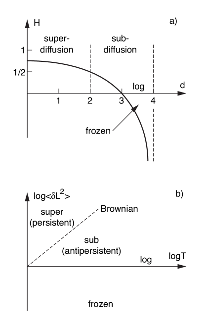
Figure 17: In a) we plot the Hurst exponent as function of $d$. In b) we depict in a log-log plot the mean square deviation $\langle\delta L^{2}\rangle$ as a function of $T$.

VIII Upper critical dimension

In addition to the scaling properties in the rough phase characterized by a strong coupling fixed point which in 1D yields $z=3/2$, a major open problem is the existence of an upper critical dimension. On the basis of the singular behavior of perturbation theory and the beta function in a Callan-Symanzik RG scheme Wiese (1998), the mapping to directed polymers Lässig and Kinzelbach (1997), and mode coupling arguments Colaiori and Moore (2001a), it has been conjectured that $d=4$ is an upper critical dimension for the KPZ equation. The behavior above 4D presumed to be complex and maybe glassy is, however, not well understood.

Here we address the issue of an upper critical dimension within the context of the weak noise approach and associate it with the existence of growth modes. This is not a scaling argument but based on the assumption that the growth mechanism and strong coupling features of the KPZ equation depend on the existence of propagating localized growth modes across the system. In Sec. V the numerical analysis of the bound state solution of the NLSE indicated that for $d\geq 4$ the solution is absent. This suggest that $d=4$ within the present interpretation plays the role of an upper critical dimension. Below we amplify this argument by means of an application of Derrick’s theorem.

VIII.1 Derricks theorem

Derrick’s theorem Derrick (1964), see also Refs. Rajaraman (1987); Coleman (1985); Dodd et al. (1982), states that for a wide class of nonlinear wave equation there does not exist stable localized time-independent solutions with finite energy in dimensions greater than one. The theorem effective rules out soliton-like solutions to Lagrangian field theories in higher dimensions. Here we sketch the simple arguments in Derrick’s theorem.

Let us consider the generic Hamiltonian

$$H=\frac{1}{2}\int d^{d}x~{}[(\nabla\phi)^{2}+V(\phi)+p^{2}],$$ (188)

for a scalar field $\phi$ in $d$ dimensions. $V(\phi)$ is the potential and $p$ the momentum. From the Hamilton equations of motion $\partial\phi/\partial t=\delta H/\delta p$ and $\partial p/\partial t=-\delta H/\delta\phi$ we readily obtain $\partial\phi/\partial t=p$ and $\partial p/\partial t=\nabla^{2}\phi-(1/2)V^{\prime}(\phi)$, or eliminating $p$, the nonlinear wave equation

$$\frac{\partial^{2}\phi}{\partial t^{2}}=\nabla^{2}\phi-\frac{1}{2}V^{\prime}(\phi).$$ (189)

For a stationary field $\phi({\bf r})$ the energy is given by

$$E=\frac{1}{2}\int d^{d}x~{}[(\nabla\phi)^{2}+V(\phi)],$$ (190)

and the Euler equation

$$\nabla^{2}\phi=\frac{1}{2}V^{\prime}(\phi),$$ (191)

follows from the variational principle

$$\frac{\delta E}{\delta\phi({\bf r})}=0.$$ (192)

To ensure stability we, moreover, require that the matrix

$$\frac{\delta^{2}E}{\delta\phi({\bf r})\delta\phi({\bf r}^{\prime})}=[-\nabla^{2}+\frac{1}{2}V^{\prime\prime}(\phi)]\delta({\bf r}-{\bf r}^{\prime}),$$ (193)

is positive definite, i.e., $\delta^{2}E\geq 0$. Performing a constrained minimization corresponding to a dilatation or scale transformation

$$\phi_{\mu}({\bf r})=\phi(\mu{\bf r}),$$ (194)

and introducing the notation

$$K=\frac{1}{2}\int d^{d}x(\nabla\phi)^{2},$$ (195)

$$I=\frac{1}{2}\int d^{d}xV(\phi),$$ (196)

$$E_{\mu}=\frac{1}{2}\int d^{d}x[(\nabla\phi_{\mu})^{2}+V(\phi_{\mu})],$$ (197)

we obtain by substitution the relation

$$E_{\mu}=\mu^{2-d}K+\mu^{-d}I.$$ (198)

Implementing the variational principle $\delta E/\delta\phi=0$ as a constrained variation $dE_{\mu}/d\mu|_{\mu=1}=0$ we infer the identity

$$(2-d)K=I.$$ (199)

Moreover, the stability matrix $\delta^{2}E/\delta\phi^{2}\rightarrow d^{2}E_{\mu}/d\mu^{2}|_{\mu=1}$ is given by

$$\left(\frac{d^{2}E_{\mu}}{d\mu^{2}}\right)_{\mu=1}=(2-d)(1-d)K+d(d+1)I.$$ (200)

Inserting Eq. (199) we finally obtain

$$\left(\frac{d^{2}E_{\mu}}{d\mu^{2}}\right)_{\mu=1}=2(2-d)K.$$ (201)

Since $K>0$ we must require $d<2$ in order to obtain a stable stationary solution.

This is the basic result of Derrick’s theorem: The existence of stable localized configurations $\phi({\bf r})$, i.e., with a finite norm, as solutions to nonlinear field equations, is only ensured below 2D. Derrick’s theorem is a no-go theorem which effectively rules out stable soliton-like solutions in higher dimension.

VIII.2 Nonexistence of growth modes above $d=4$

Here we address the issue of the existence of growth modes by an application of Derrick’s theorem to the NLSE, see also Refs. Rasmussen and Rypdal (1986); Rypdal and Rasmussen (1986). In the context of the NLSE (83) the issue is not stability but existence of bound states. Here the energy functional can be expressed in the form

$$E=K+\frac{1}{2}k^{2}N-\frac{k_{0}^{2}}{4}I,$$ (202)

where $K$ is the bending energy, $N$ the norm, and $I$ the interaction,

$$K=\frac{1}{2}\int d^{d}x(\nabla w)^{2},$$ (203)

$$N=\int d^{d}xw^{2},$$ (204)

$$I=\int d^{d}xw^{4},$$ (205)

and the NLSE

$$\nabla^{2}w=k^{2}w-k_{0}^{2}w^{3},$$ (206)

follows from the variation $\delta E/\delta w=0$.

In order to establish the bound we need two identities. The first identity is obtained by multiplying the NLSE by $w$ and integrating over space yielding

$$2K+k^{2}N-k_{0}^{2}I=0.$$ (207)

The second identity is obtained by constrained minimization. Subject to the scale transformation $w({\bf r})\rightarrow w(\mu{\bf r})$ we infer $K\rightarrow\mu^{d-2}K$, $N\rightarrow\mu^{d}N$, and $I\rightarrow\mu^{d}I$, and applying constrained minimization $dE/d\mu|_{\mu=1}=0$ we infer the second identity

$$(d-2)K+\frac{k^{2}}{2}dN-\frac{k_{0}^{2}}{4}dI=0.$$ (208)

Eliminating the bending term $K$ from the two identities we obtain

$$k^{2}N=\frac{k_{0}^{2}}{4}(4-d)I.$$ (209)

Since $N>0$, and $I>0$ it follows that $d<4$ in order for a bound state to exist.

This completes the proof of the nonexistence of bound states and thus growth modes for the KPZ equation in the Cole-Hopf formulation in dimensions larger than 4. The proof corroborates the numerical analysis of the bound state solution.

IX Summary and Conclusion

In the present paper we have extended the weak noise approach, previously applied in detail to the 1D noisy Burgers equation, to the KPZ equation in higher dimensions. Three issues have been addressed: i) kinetic pattern formation, ii) anomalous diffusion and scaling, and iii) the upper critical dimension.

i) The weak noise WKB formulation allows a classical interpretation of the pattern formation in the KPZ equation in the sense that the growth of the interface is interpreted as a dynamical deterministic network of propagating localized growth modes. The growth modes play the role of elementary excitations and are analogous to the vortex structures in the Kosterlitz-Thouless theory or hedgehog structures in the ferromagnet, see Ref. Chaikin and Lubensky (1995). The imposed network structure expresses the strong coupling features. Superimposed on the network is a gas of subdominant extended diffusive modes corresponding to the EW universality class. The dynamical evolution of the network together with the diffusive modes defines the kinetic pathways from an initial configuration to a final configuration. Within the canonical weak noise scheme the network is endowed with dynamical attributes, it carries energy, momentum, and action. Here the action $S$ plays the particular role of a weight function in determining the transition probability $P\propto\exp(-S/\Delta)$, $\Delta$ is the noise strength, for a specific kinetic pathway.

ii) The weak noise method gives access to the scaling properties of the KPZ equation. The nonperturbative character of the WKB approximation implies that strong coupling features might be accessible. This is in fact the case in 1D where the exact scaling exponents can be retrieved from the dispersion law for the growth modes and the structure of the stationary zero-energy submanifold. In higher D the stationary submanifold is not know and only limited scaling results are available in the dipole sector. In the dipole or pair mode sector, corresponding to a dilute gas of dipole modes, the stochastic interpretation implies that the pair modes perform random walk with Hurst exponent $H=(3-d)/(4-d)$. In 1D the interface grows stochastically with $H=2/3$, corresponding to persistent super diffusion; in 2D, the lower critical dimension, $H=1/2$, corresponding to ordinary Brownian motion; in 3D we have $H=0$, equivalent to logarithmic antipersistent subdiffusion; finally, in 4D, the conjectured upper critical dimension, $H$ diverges, corresponding to an arrested or frozen interface. Formally, the dynamic exponent for the dipole sector is given by $z=1/H=(4-d)/(3-d)$. In 1D we recover the well-known result $z=3/2$; in 2D we have $z=2$ which is the weak coupling result. In 3D the dynamic exponent diverges; in 4D we have $z=0$. We believe that the behavior of $z$ above $d=2$ is an artifact associated with the dipole sector; it does not reflect the true scaling behavior of the KPZ problem.

iii) The issue of an upper critical dimension for the KPZ equation has been much debated. Dynamical renormalization group arguments indicates $d=4$ as the upper critical dimension; numerical simulations, on the other hand, suggest an infinite upper critical dimension. Here we associate the upper critical dimension with the existence of growth modes. This is not a scaling argument but rather associated with the idea that in the absence of a network of localized growth modes there is no clear mechanism for the growth of the interface. Above 4D the interface is, of course, still governed by the nonlinear KPZ equation but we lack insight into the actual growth mechanism if any.

This paper constitutes our present understanding of the KPZ equation within the weak noise WKB approach. However, many open problems remain.

i)Dynamical network: We have only analyzed the network in terms of the asymptotic form of the growth modes. A detailed analysis of the long time behavior requires further analysis of the field equations in order to understand collisions and coalescence of growth modes. Moreover, the analysis of the linear diffusive modes and their interaction with the growth modes is incomplete. Further analysis is required in order to determine the transition probabilities for specific kinetic pathways.

ii)Scaling: In order to determine the scaling properties we need to determine the stationary zero-energy manifold yielding the stationary distribution. This is only possible in 1D; in higher D the stationary submanifold is unknown and we only have scaling results for the dipole sector.

iii)Dynamic renormalization group: The present approach is based on the noise strength being the nonperturbative small parameter in the problem. In that sense the method is not a scaling approach. It is unclear how to relate the weak noise approach to the dynamic renormalization group scheme.

iv) Directed polymers: An important element in our understanding of the KPZ equation is the mapping to directed polymers in a random medium. The relationship between the growth modes and the wandering of polymers is an open problem.

In conclusion, the present nonperturbative weak noise scheme represents an alternative angle of approach to the KPZ equation and similar noise-driven problems. We emphasize that the method is not a scaling approach based on expansions about critical dimensions, but rather identifies the noise strength as the small parameter in the problem. Moreover, the method is not based on perturbation theory but on an asymptotic nonperturbative WKB or eikonal approximation.

Appendix A Weak noise approach to simple random walk and the overdamped oscillator

A.1 Random Walk

Simple 1D random walk is described by the Langevin equation

$$\frac{dx}{dt}=\eta(t)~{},~{}~{}~{}\langle\eta(t)\eta(0)\rangle=\Delta\delta(t),$$ (210)

corresponding to vanishing drift $F=0$. From the weak noise scheme we obtain the Hamiltonian

$$H=\frac{1}{2}p^{2},$$ (211)

and the equations of motion

$$\frac{dx}{dt}=p~{},~{}~{}\frac{dp}{dt}=0,$$ (212)

with solution from $x^{i}$ to $x$ in time $T$,

$$x-x^{i}=p_{0}T~{},~{}~{}p=p_{0}.$$ (213)

In the weak noise scheme random walk corresponds to free particle propagation. The action is

$$S=\frac{1}{2}p_{0}^{2}T,$$ (214)

and we infer the well-known distribution Risken (1989)

$$P(x,T)\propto\exp\left[-\frac{(x-x^{i})^{2}}{2\Delta T}\right],$$ (215)

for the spread of random walk, i.e., the mean square displacement $\langle(x-x^{i})^{2}\rangle\propto\Delta T$. The transient zero-energy manifold is given by $H=(1/2)p_{0}^{2}=0$. There is no stationary zero-energy manifold and no saddle point in accordance with the fact that random walk does not attain a stationary state. In Fig. 18 we show the simple random walk phase space.

Figure 18: The $(x,p)$ phase space for the random walk case. The transient zero-energy manifold is given by $p=0$.

A.2 Overdamped oscillator

The overdamped oscillator in 1D is described by the Langevin equation

$$\frac{dx}{dt}=-\gamma x+\eta(t)~{},~{}~{}~{}\langle\eta(t)\eta(0)\rangle=\Delta\delta(t),$$ (216)

corresponding to the drift $F=2\gamma x$. We obtain the Hamiltonian

$$H=\frac{1}{2}p^{2}-\gamma px=\frac{1}{2}p(p-2\gamma x),$$ (217)

and ensuing equations of motion

$$\frac{dx}{dt}=-\gamma x+p~{},~{}~{}\frac{dp}{dt}=\gamma p,$$ (218)

with solution from $x^{\text{i}}$ to $x$ in time $T$,

$$x(t)=\frac{x\sinh\gamma t+x^{\text{i}}\sinh\gamma(T-t)}{\sinh\gamma T},$$ (219)

$$p(t)=\gamma e^{\gamma t}\frac{x-x^{i}e^{-\gamma T}}{\sinh\gamma t}.$$ (220)

From Eqs. (218) we have $d^{2}x/dt^{2}=\gamma^{2}x$ and the overdamped noise-driven oscillator thus corresponds to the motion of a particle in an inverted harmonic potential.

The zero-energy manifold $H=0$ is composed of the transient submanifold $p=0$ and the stationary submanifold $p=2\gamma x$ intersecting at the saddle point $(x,p)=(0,0)$. From the action $S=(1/2)\int_{0}^{T}dt~{}p(t)^{2}$ we obtain the familiar distribution Risken (1989)

$$P(x,T)\propto\exp\left[-\frac{\gamma}{\Delta}\frac{(x-x^{i}e^{-\gamma T})^{2}}{1-e^{-2\gamma T}}\right].~{}~{}~{}~{}$$ (221)

For $T\rightarrow\infty$ we infer the stationary distribution

$$P_{0}(x)\propto\exp\left[-\frac{\gamma x^{2}}{\Delta}\right].$$ (222)

In Fig. 19 we have shown the phase space for the overdamped oscillator.

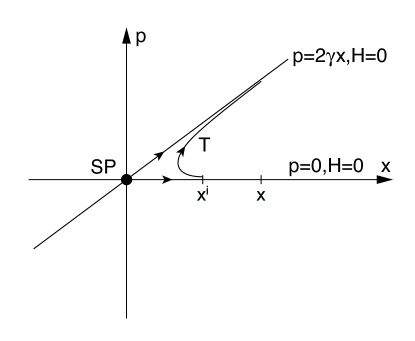
Figure 19: The $(x,p)$ phase space for the overdamped oscillator case. The transient zero-energy manifold is given by $p=0$ and the stationary zero-energy manifold by $p=2\gamma x$. The manifolds intersect at the saddle point (SP) $(x,p)=(0,0)$.

We note that in both the random walk case and the overdamped oscillator case, the weak noise method gives the exact and familiar results; quite similar to the corresponding calculations in the WKB approximation in quantum mechanics.

References

- Nelson (2003) P. Nelson, Biological Physics (Freeman, New York, 2003).
- Chaikin and Lubensky (1995) P. M. Chaikin and T. C. Lubensky, Principles of condensed matter physics (Cambridge University Press, Cambridge, 1995).
- Binney et al. (1992) J. J. Binney, N. J. Dowrick, A. J. Fisher, and M. E. J. Newman, The Theory of Critical Phenomena (Clarendon Press, Oxford, 1992).
- Cross and Hohenberg (1994) M. C. Cross and P. C. Hohenberg, Rev. Mod. Phys 65, 851 (1994).
- Barabasi and Stanley (1995) A. L. Barabasi and H. E. Stanley, Fractal Concepts in Surface Growth (Cambridge University Press, Cambridge, 1995).
- Kardar et al. (1986) M. Kardar, G. Parisi, and Y. C. Zhang, Phys. Rev. Lett. 56, 889 (1986).
- Medina et al. (1989) E. Medina, T. Hwa, M. Kardar, and Y. C. Zhang, Phys. Rev. A 39, 3053 (1989).
- Krug (1997) J. Krug, Adv. Phys. 46, 139 (1997).
- Krug et al. (1992) J. Krug, P. Meakin, and T. Halpin-Healy, Phys. Rev. A 45, 638 (1992).
- Family (1990) F. Family, A168, 561 (1990).
- Halpin-Healy and Zhang (1995) T. Halpin-Healy and Y. C. Zhang, Phys. Rep. 254, 215 (1995).
- Forster et al. (1976) D. Forster, D. R. Nelson, and M. J. Stephen, Phys. Rev. Lett. 36, 867 (1976).
- Forster et al. (1977) D. Forster, D. R. Nelson, and M. J. Stephen, Phys. Rev. A 16, 732 (1977).
- E and Vanden-Eijnden (2000) W. E and E. Vanden-Eijnden, Comm. Pure App. Math 53, 0825 (2000).
- Woyczynski (1998) W. A. Woyczynski, Burgers–KPZ Turbulence (Springer–Verlag, New York, 1998).
- Burgers (1929) J. M. Burgers, Proc. Roy. Neth. Acad. Soc. 32, 414, 643, 818 (1929).
- Burgers (1974) J. Burgers, The Nonlinear Diffusion Equation (Riedel, Boston, 1974).
- Saffman (1968) P. Saffman, Topics in Nonlinear Physics, ed. N.J. Zabusky (Springer, New York, 1968).
- Jackson (1990) E. Jackson, Perspectives of nonlinear dynamics (Cambridge University Press, Cambridge, 1990).
- Whitham (1974) G. B. Whitham, Nonlinear Waves (Wiley, New York, 1974).
- Zeldovitch (1972) Y. Zeldovitch, Astron. Astrophys 8, 84 (1972).
- Fogedby (1998a) H. C. Fogedby, Phys. Rev. E 57, 2331 (1998a).
- Fogedby et al. (1995) H. C. Fogedby, A. B. Eriksson, and L. V. Mikheev, Phys. Rev. Lett. 75, 1883 (1995).
- Fogedby (1998b) H. C. Fogedby, Phys. Rev. E 57, 4943 (1998b).
- Martin et al. (1973) P. C. Martin, E. D. Siggia, and H. A. Rose, Phys. Rev. A 8, 423 (1973).
- Baussch et al. (1976) R. Baussch, H. K. Janssen, and H. Wagner, 24, 113 (1976).
- Janssen (1976) H. K. Janssen, Z. Phys. B 23, 377 (1976).
- DeDominicis and Peliti (1978) C. DeDominicis and L. Peliti, Phys. Rev. B 18, 353 (1978).
- Fogedby (1999a) H. C. Fogedby, Phys. Rev. E 59, 5065 (1999a).
- Freidlin and Wentzel (1998) M. I. Freidlin and A. D. Wentzel, Random Perturbations of Dynamical Systems (2nd ed. Springer, New York, 1998).
- Graham (1989) R. Graham, Noise in nonlinear dynamical systems, Vol 1, Theory of continuous Fokker-Planck systems, eds. F. Moss and P. E. V. McClintock (Cambridge University Press, Cambridge, 1989).
- Lichtenberg and Lieberman (1983) A. Lichtenberg and M. Lieberman, Regular and Stochastic Motion (Springer-Verlag, New York, 1983).
- Ott (1993) E. Ott, Chaos in Dynamical Systems (Cambridge University Press, Cambridge, 1993).
- Schuster (1989) H. G. Schuster, Deterministic Chaos, An Introduction (VCH Verlagsgesellschaft mbH, Weinheim, 1989), 2nd ed.
- Fogedby (1998c) H. C. Fogedby, Phys. Rev. Lett. 80, 1126 (1998c).
- Fogedby (1999b) H. C. Fogedby, Phys. Rev. E 60, 4950 (1999b).
- Fogedby (2001a) H. C. Fogedby, Europhys. Lett 56, 492 (2001a).
- Fogedby (2001b) H. C. Fogedby, Eur. Phys. J. B 20, 153 (2001b).
- Fogedby and Brandenburg (2002) H. C. Fogedby and A. Brandenburg, Phys. Rev. E 66, 016604 (2002).
- Fogedby (2002a) H. C. Fogedby, J. Phys.: Condens. Matter 14, 1557 (2002a).
- Fogedby (2002b) H. C. Fogedby, Physica A 314, 182 (2002b).
- Fogedby (2003a) H. C. Fogedby, Phys. Rev. E 68, 026132 (2003a).
- Family (1986) F. Family, J. Phys. A 19, L441 (1986).
- Wiese (1998) K. J. Wiese, J. Stat. Phys. 93, 143 (1998).
- Lässig and Kinzelbach (1997) M. Lässig and H. Kinzelbach, Phys. Rev. Lett. 78, 903 (1997).
- Colaiori and Moore (2001a) F. Colaiori and M. A. Moore, Phys. Rev. Lett. 86, 3946 (2001a).
- Derrick (1964) G. H. Derrick, J. Math. Phys. 5, 1252 (1964).
- Fogedby (2005) H. C. Fogedby, Phys. Rev. Lett. 94, 195702 (2005).
- Huse et al. (1985) D. A. Huse, C. L. Henley, and D. S. Fisher, Phys. Rev. Lett. 55, 2924 (1985).
- Edwards and Wilkinson (1982) S. F. Edwards and D. R. Wilkinson, Proc. Roy. Soc. London A 381, 17 (1982).
- Majaniemi et al. (1996) S. Majaniemi, T. Ali-Nissila, and J. Krug, Phys. Rev. B 53, 8071 (1996).
- Cole (1951) J. D. Cole, Quart. Appl. Math. 9, 22 (1951).
- Hopf (1950) E. Hopf, Comm. Pure Appl. Math. 3, 201 (1950).
- Kardar (1987) M. Kardar, Nucl. Phys. B 290, 582 (1987).
- Family and Vicsek (1985) F. Family and T. Vicsek, J. Phys. A 18, L75 (1985).
- Wiese (1997) K. J. Wiese, Phys. Rev. E 56, 5013 (1997).
- Schwartz and Edwards (1992) M. Schwartz and S. F. Edwards, 20, 301 (1992).
- Bouchaud and Cates (1993) J. P. Bouchaud and M. E. Cates, Phys. Rev. E 47, R1455 (1993).
- Doherty et al. (1994) J. P. Doherty, M. A. Moore, J. M. Kim, and A. J. Bray, Phys. Rev. Lett. 72, 2041 (1994).
- Moore et al. (1995) M. A. Moore, T. Blum, J. P. Doherty, M. Marsili, J. P. Bouchaud, and P. Claudin, Phys. Rev. Lett. 74, 4257 (1995).
- Lässig (1998) M. Lässig, Phys. Rev. Lett. 80, 2366 (1998).
- Marinari et al. (2000) E. Marinari, A. Pagnani, and G. Parisi, J. Phys. A 33, 8181 (2000).
- Marinari et al. (2002) E. Marinari, A. Pagnani, G. Parisi, and Z. Racz, Phys. Rev. E 65, 026136 (2002).
- (64) (????).
- Beccaria and Curci (1994) M. Beccaria and G. Curci, Phys. Rev. E 50, 4560 (1994).
- Lässig (1995) M. Lässig, Nucl. Phys. B 448, 559 (1995).
- Kim and Kosterlitz (1989) J. M. Kim and J. M. Kosterlitz, Phys. Rev. Lett. 62, 2289 (1989).
- Wolf and Kertész (1997) D. E. Wolf and J. Kertész, Europhys. Lett 4, 651 (1997).
- Bhattacharjee (1998) J. K. Bhattacharjee, J. Phys. A 31, L93 (1998).
- Colaiori and Moore (2001b) F. Colaiori and M. A. Moore, Phys. Rev. E 63, 057103 (2001b).
- Onsager and Machlup (1953) L. Onsager and S. Machlup, Phys. Rev. 91, 1505 (1953).
- Machlup and Onsager (1953) S. Machlup and L. Onsager, Phys. Rev. 91, 1512 (1953).
- Graham and Tél (1984a) R. Graham and T. Tél, J. Stat. Phys. 35, 729 (1984a).
- Graham and Tél (1984b) R. Graham and T. Tél, Phys. Rev. Lett. 52, 9 (1984b).
- Graham et al. (1985) R. Graham, D. Roekaerts, and T. Tél, Phys. Rev. A 31, 3364 (1985).
- Dykman (1990) M. I. Dykman, Phys. Rev. A 42, 2020 (1990).
- Bray and McKane (1989) A. J. Bray and A. J. McKane, Phys. Rev. Lett. 62, 493 (1989).
- Maier and Stein (1996) R. S. Maier and D. L. Stein, J. Stat. Phys. 83, 291 (1996).
- Maier and Stein (2001) R. S. Maier and D. L. Stein, Phys. Rev. Lett. 87, 270601 (2001).
- Aurell and Sneppen (2002) E. Aurell and K. Sneppen, Phys. Rev. Lett. 88, 048101 (2002).
- Stratonovich (1963) R. L. Stratonovich, Topics in the Theory of Random Noise (Gordon and Breach, New York, 1963).
- Risken (1989) H. Risken, The Fokker-Planck Equation (Springer-Verlag, Berlin, 1989).
- Reimann (2002) P. Reimann, Physics Reports 361, 57 (2002).
- Landau and Lifshitz (1959a) L. Landau and E. Lifshitz, Quantum Mechanics (Pergamon Press, Oxford, 1959a).
- Goldstein (1980) H. Goldstein, Classical Mechanics (Addison-Wesley Publishing Company, Inc., Reading, Massachusetts, 1980).
- Arnold (1983) V. Arnold, Mathematical Methods of Classical Mechanics (Springer-Verlag, New York, 1983).
- Reichl (1987) L. E. Reichl, The Transition to Chaos (Springer-Verlag, New York, 1987).
- Scott (1999) A. Scott, Nonlinear Science (Oxford University Press, Oxford, 1999), 1st ed.
- Landau and Lifshitz (1959b) L. Landau and E. Lifshitz, Mechanics (Pergamon Press, Oxford, 1959b).
- Coleman (1977) S. Coleman, The Use of Instantons, in ”Aspects of Symmetry” (Cambridge University Press, Cambridge, 1977).
- Fogedby and Poukaradze (2002) H. C. Fogedby and V. Poukaradze, Phys. Rev. E 66, 021103 (2002).
- Fogedby (2003b) H. C. Fogedby, Phys. Rev. E 68, 051105 (2003b).
- Fogedby et al. (2003) H. C. Fogedby, J. Hertz, and A. Svane, Europhys. Lett 62, 795 (2003).
- Fogedby et al. (2004) H. C. Fogedby, J. Hertz, and A. Svane, Phys. Rev. E 70, 031105 (2004).
- Fogedby (1980) H. C. Fogedby, Theoretical Aspects of Mainly Low Dimensional Magnetic Systems (Springer-Verlag, New York, 1980).
- Lebedev (1972) N. N. Lebedev, Special functions and their applications (Dover Publications, New York, 1972).
- Pethick and Smith (2002) C. J. Pethick and H. Smith, Bose-Einstein Condensation in Dilute Gases (Cambridge University Press, Cambridge, 2002).
- Chiao et al. (1964) R. Y. Chiao, E. Gamire, and C. H. Townes, Phys. Rev. Lett. 13, 479 (1964).
- Finkelstein et al. (1951) R. Finkelstein, R. LeLevier, and R. Ruderman, Phys. Rev. 83, 326 (1951).
- Das (1993) A. Das, Field Theory - A Path Integral Approach (World Scientific, Singapore, 1993).
- Rajaraman (1987) R. Rajaraman, Solitons and Instantons (North-Holland, Amsterdam, 1987).
- Landau and Lifshitz (1960) L. Landau and E. Lifshitz, Electrodynamics of Continuous Media (Pergamon Press, Oxford, 1960).
- Feder (1988) J. Feder, Fractals (Plenum Press, New York, 1988).
- Coleman (1985) S. Coleman, Aspects of Symmetry (Cambridge University Press, London, 1985).
- Dodd et al. (1982) R. K. Dodd, J. C. Eilbeck, J. D. Gibbon, and H. C. Morris, Solitons and Nonlinear Wave Equations (Academic Press, New York, 1982).
- Rasmussen and Rypdal (1986) J. J. Rasmussen and K. Rypdal, Physica Scripta 33, 481 (1986).
- Rypdal and Rasmussen (1986) K. Rypdal and J. J. Rasmussen, Physica Scripta 33, 498 (1986).