KINETICS OF 2D ELECTRONS IN THE MAGNETIC FIELD IN THE PRESENCE OF MICROWAVE RADIATION. RESPONSE OF A NON-EQUILIBRIUM SYSTEM TO A WEAK MEASUREMENT FIELD

Abstract

Kinetics of spatially uniform distribution of 2D electrons in crossed electric and magnetic fields in the presence of microwave radiation has been studied. In the present model the contribution from the microwave radiation and the effects of Landau quantization are considered exactly, while scattering is treated perturbatively. Here Landau—Floquet states interact with the impurity potential that causes transitions between them. The linear response of a non-equilibrium system to a weak measurement field has been considered for the case when the non-equilibrium state of the carriers can be described by the average values of the total energy and the number of particles.

I Introduction

In two-dimensional electron systems (2DES) with high ($\sim 10^{7}\ \mathrm{cm^{2}/Vs}$) mobility, the magnetoresistance exhibits strong oscillations in pre-Shubnikov interval of magnetic fields under microwave irradiation Zudov03 ; Mani02 . The parameter that governs those oscillations is the ratio of the radiation frequency $\omega$ to the cyclotron frequency $\omega_{c}$. The maxima of the magnetoresistance are observed at $\omega/\omega_{c}=j-1/4$, where $j$ takes integer values. The resistance of the sample is minimal at $\omega/\omega_{c}=j+1/4$, and with sufficiently intensive radiation zero-resistance states are observed.

Let’s mention the important features of the above-mentioned experiments. The effect is observed under the conditions: $\hbar/\tau\ll T\simeq\hbar\omega_{c}\leq\hbar\omega\ll\zeta$, from which one can conclude that its nature is quasiclassical. Here $\tau$ is the momentum relaxation time, $\omega\geq\omega_{c}$ are the radiation frequency and the cyclotron frequency, respectively, $\zeta$ is the Fermi energy, $T$ is the temperature expressed in units of energy.

Currently, there exist a sufficiently large number of theoretical papers (Durst03 ; Shi03 ; Mikhailov03 ; Dmitriev0310 ; Dmitriev0304 ; Volkov03 , see also Vavilov04 and references therein) in which various aspects of the observed phenomena are considered. It is necessary to note that the possibility of the existence of negative-resistance states was first predicted in Ryzhii68 . Some of the models are based upon the influence of the microwave radiation upon the processes of scattering an electron along the weak dc electric field or in the opposite direction. There are also alternative explanations that relate the observed phenomena with non-trivial dependence of the non-equilibrium distribution function upon the energy, that acquires oscillating character under the effect of the microwave radiation. The schemes described above presume that only bulk effects are responsible for the observed phenomena. Other models are possible. E.g., the scenario proposed in Mikhailov03 says that two mechanisms are actually important. One of them leads to a resonance at the magnetoplasmon frequency and is of the bulk origin. The second one is related to the development of drift plasma instability at the edge of the sample. Both the proposed models and the predictions that follow from them still require additional experimental validation.

In this paper, in order to explain the observed conductivity oscillations, we present a model that incorporates contributions from Landau quantization and microwave irradiation (in long-wavelength limit) exactly, without the use of perturbation theory. Electron scattering upon impurities is considered perturbatively. With respect to Landau—Floquet states, impurities act as a coherent oscillating field that causes transitions which are essential for reproducing the oscillating magnetoresistance behavior. This problem is a classical variant of the theory of non-equilibrium system response to a weak measuring field. Indeed, under microwave irradiation, in the system under consideration a non-equilibrium state is formed. The task is to find the response of such possibly strongly non-equilibrium system to a weak measuring field.

It is worth mentioning that the theory of linear reaction upon external mechanical perturbations is currently well-established. Within this approach, the kinetic coefficients are expressed in terms of the equilibrium correlation functions. However, the situation changes radically if it is required to find the response of a system that is already out of the equilibrium, to an additional measurement field. Problems of this kind are usually solved with the help of the method of kinetic equations. We shall apply the theory of linear response of a non-equilibrium system to a weak measurement field for analysis of the transport phenomena for 2D charge carriers under microwave irradiation.

Our results depict strong oscillations of $\rho_{xx}$ with negative resistance states. It has been found that that the microwave-induced correction to $\rho_{xx}$ vanishes when $\epsilon=\omega/\omega_{c}=j$, $j$ is an integer. Oscillations have minima at $\epsilon=j+\delta$ and maxima at $\epsilon=j-\delta$, where $\delta\approx 1/5$. The calculations have been carried out for various polarizations of microwave electric field. The role of the mobility of the carriers for the magnetoresistance oscillations has been studied. It has been shown that magnetoresistance oscillations should still be observable in the lower-mobility samples if one increases the microwave radiation frequency. A role of multiphoton process in this phenomenon can also be relatively easily studied using the described approach.

The article is organized in the following way. In section II, the canonical transformation of the Hamiltonian is considered. This allows us to avoid the direct analysis of the system’s reaction upon the ac electric field of the microwave radiation that is not necessarily a weak perturbation. Section III contains a short introduction into the theory of the linear response of a non-equilibrium system. This theory is applied to the canonically-transformed system. In the same section, the main results for the magnetoconductivity tensor are expressed. Finally, the results of the numerical analysis are presented in section IV, followed by the conclusion.

II Canonical transformation

Let’s consider a system of 2D charge carriers and scatterers in a conducting crystal under effect of dc magnetic $(0,0,B)$, dc electric $\vec{E}=(E_{x},0,0)$ and ac electric $\vec{E}(t)=(E_{x}(t),E_{y}(t),0)$ fields. The Hamiltonian of such system is can be written in the following form:

$$H(t)=H_{e}+H_{v}+H_{ev}+H_{ef}(t)+H^{0}_{ef},$$ (1)

where

$$H_{e}=\sum_{i}\frac{P_{i}^{2}}{2m}=\sum_{i}\frac{(\vec{p}_{i}-(e/c)\vec{A}_{i})^{2}}{2m}=\sum_{i}\frac{1}{4m}(P^{+}_{i}P^{-}_{i}+P^{-}_{i}P^{+}_{i})$$ (2)

is the Hamiltonian of free charge carriers in the magnetic field, $m$ is the effective mass, $e$ is the electron charge, $P^{\alpha}_{i}$ is a component of kinetic momentum of electrons, and

$$P^{\pm}=P_{x}\pm iP_{y},\qquad[P^{+},P^{-}]=2m\hbar\omega_{c},\quad[P^{\pm},H_{e}]=\pm\hbar\omega_{c}P^{\pm}.$$

$\omega_{c}=|e|B/mc$ is the cyclotron frequency of electrons.

$$\vec{A}=-\frac{1}{2}[\vec{r}\times\vec{B}]$$

is the vector potential. $H_{v}$ is the Hamiltonian of the lattice, $H_{ev}$ is the Hamiltonian of the interaction of electrons with scatterers (in this case, impurities are considered). $H_{ef}(t)$ is the Hamiltonian of interaction of conducting electrons with the ac electric field, and $H^{0}_{ef}$ describes the interaction with the external dc electric field $\vec{E}$ response to which is what we are interested in.

$$H^{0}_{ef}=-eE^{\alpha}\sum_{i}x^{\alpha}_{i}.$$ (3)

In the laboratory frame of reference, evolution of the state of a free 2D electron is described by Schrödinger equation:

$$\{i\frac{\partial}{\partial t}-H_{0}(t)\}\psi(\vec{r},t)=\{i\frac{\partial}{\partial t}-H_{0}+H_{ef}(t)\}\psi(\vec{r},t)=0.$$ (4)

Here $H_{0}(t)$ is the Hamiltonian of an electron without interaction with scatterers, $\psi(\vec{r},t)$ is the wave function describing the electron state. Let’s perform a time-dependent canonical transformation $W_{t}$ that would exclude the ac electric field from the Schrödinher equation, i. e.

$$W^{\dagger}_{t}\{i\frac{\partial}{\partial t}-H_{0}(t)\}W_{t}=i\frac{\partial}{\partial t}-H_{0}.$$ (5)

If such a transformation is done, then, obviously, any solution of Eq. (4) can be represented as a result of canonical transformation of the corresponding solution without the ac electric field, i. e.

$$\Psi(\vec{r},t)=W_{t}\psi(\vec{r},t).$$ (6)

The unitary transformation of the state vector (6) is in fact a change of the reference frame from the laboratory one to the one moving with the time-dependent velocity ${\dot{\vec{\xi}}(t)}=\partial\vec{\xi}/\partial t$. Thus, it corresponds to the shift of coordinates $\vec{r}\rightarrow\vec{r}+\vec{\xi}(t)$ and momenta $\vec{p}\rightarrow\vec{p}+m{\dot{\vec{\xi}}(t)}$.

Note that, in the presence of magnetic field, the translation in the coordinate space should be considered as the operation of “magnetic translation”, defined as

$$T_{\vec{\xi}}\Psi(\vec{r})=\exp\{i\frac{e}{c}\vec{A}(\vec{\xi})\cdot\vec{r}\}\exp(-i\vec{\xi}\cdot\vec{p})\Psi(\vec{r}),$$ (7)

where $\vec{A}(\vec{\xi})=(\vec{B}\times\vec{\xi})/2$ is the vector potential of the external magnetic field in the symmetric gauge: $\vec{A}=(-\frac{1}{2}yB,\frac{1}{2}xB,0)$. The operator $W_{t}$ that defines the unitary (canonical) transformation can be represented in the following form:

$$W_{t}=\exp\{i\theta(t)\}\exp\{-i\vec{\xi}\cdot\vec{p}\}\exp\{i(m\vec{\dot{\xi}}+\frac{e}{2c}\vec{B}\times\vec{\xi})\cdot\vec{r}\}.$$ (8)

The real-valued function $\theta(t)$ and parameters $\vec{\xi}$, $\vec{\dot{\xi}}$ should be chosen appropriately for Eq. (5) to be fulfilled. This condition allows us to cast the unitary operator $W_{t}$ to the following form:

$$W_{t}=\exp\{i\int\limits^{t}L(\tau,\vec{\xi},\vec{\dot{\xi}})d\tau\}\exp\{-i\vec{\xi}\cdot\vec{p}\}\exp\{i(m\vec{\dot{\xi}}+\frac{e}{2c}\vec{B}\times\vec{\xi})\cdot\vec{r}\}.$$ (9)

It is sufficient to let parameters $\vec{\xi}=\vec{\xi}(t)$ be the solutions of the classical equations of motion:

$$m\vec{\ddot{{\xi}}}=e\vec{E}(t)+\frac{e}{c}[\vec{\dot{\xi}}\times\vec{B}].$$ (10)

As for $\theta(t)$, it is sufficient to choose this parameter to be equal to the classical action of an electron in the ac electric field when the magnetic field is also present:

$$\theta(t)=\int\limits^{t}L(\tau,\vec{\xi},\vec{\dot{\xi}})d\tau=\int\limits^{t}[\frac{1}{2}m\vec{\dot{\xi}}^{2}+e\vec{E}(\tau)+\frac{e}{c}\vec{A}(\vec{\xi})\cdot\vec{\dot{\xi}}]d\tau.$$ (11)

During the further consideration of the problem it is convenient to introduce a new set of independent variables: coordinates of the center of the cyclotron orbit $(X_{0},Y_{0})$ and the relative motion $(\zeta,\eta)$ instead of Cartesian coordinates of electrons and the corresponding momenta:

$$\begin{array}[]{l@{\qquad\qquad}l}x=X_{0}+\zeta&\zeta=\frac{c}{eB}P_{y},\\ y=Y_{0}+\eta&\eta=-\frac{c}{eB}P_{x}\end{array}$$ (12)

that satisfy well-known commutation rules:

$$[\zeta,\eta]=-i\alpha^{2},\qquad[X_{0},Y_{0}]=i\alpha^{2},$$

$${}[\zeta,X_{0}]=[\eta,Y_{0}]=[\eta,X_{0}]=[\zeta,Y_{0}]=0,$$ (13)

where $\alpha=c\hbar/(|e|B)$ is the magnetic length.

In the new variables, the operator that defines the canonical transformation has the following form:Torres05

$$W_{t}=\exp\{i\theta_{1}(t)\}\exp\{-i\frac{y_{0}X_{0}}{\alpha^{2}}\}\exp\{i\frac{x_{0}Y_{0}}{\alpha^{2}}\}\exp\{-i\frac{x_{rel}\eta}{\alpha^{2}}\}\exp\{i\frac{y_{rel}\zeta}{\alpha^{2}}\}.$$ (14)

Here

$$\theta_{1}(t)=\theta(t)-\frac{m\omega_{c}}{2}[x_{rel}y_{rel}+x_{0}y_{rel}+x_{0}y_{0}-x_{rel}y_{0}],$$ (15)

where $x_{rel}$, $y_{rel}$, $x_{0}$, $y_{0}$ are relative coordinates and coordinates of cyclotron orbit center corresponding to the displacement vector $\vec{\xi}$.

Using the explicit expression for the operator $W_{t}$ (14), we intend to perform the transformation (5). For this, obviously, it is sufficient to know how the following operators are transformed:

$$\begin{array}[]{l@{\qquad\qquad}l}\tilde{X}_{0}\equiv W^{\dagger}_{t}X_{0}W_{t}=X_{0}+x_{0},&\tilde{Y}_{0}\equiv W^{\dagger}_{t}Y_{0}W_{t}=Y_{0}+y_{0},\\ \tilde{\zeta}\equiv W^{\dagger}_{t}\zeta W_{t}=\zeta+x_{rel},&\tilde{\eta}\equiv W^{\dagger}_{t}\eta W_{t}=\eta+y_{rel}.\end{array}$$ (16)

For Eq. (5) to hold, it is sufficient to let $x_{rel}$, $y_{rel}$, $x_{0}$, $y_{0}$ be the solutions of the classical equations of motion

$$-m\omega_{c}\dot{x}_{0}+eE_{y}=0,\qquad-m\omega_{c}\dot{y}_{rel}-m\omega_{c}^{2}x_{rel}+eE_{x}=0,$$

$$m\omega_{c}\dot{y}_{0}+eE_{x}=0,\qquad m\omega_{c}\dot{x}_{rel}-m\omega_{c}^{2}y_{rel}+eE_{y}=0.$$ (17)

Besides that,

$$\dot{\theta}_{1}=m\omega_{c}\dot{y}_{0}x_{0}+m\omega_{c}\dot{x}_{rel}y_{rel}-\frac{m\omega_{c}^{2}}{2}\{x_{rel}^{2}+y_{rel}^{2}\}+eE_{x}(x_{0}+x_{rel})+eE_{y}(y_{0}+y_{rel}).$$ (18)

Then, using (16)–(18), we obtain:

$$W^{\dagger}_{t}\{i\frac{\partial}{\partial t}-\frac{m\omega_{c}^{2}}{2}[\zeta^{2}+\eta^{2}]+eE_{x}(X_{0}+\zeta)+eE_{y}(Y_{0}+\eta)\}W_{t}=\{i\frac{\partial}{\partial t}-\frac{m\omega_{c}^{2}}{2}[\zeta^{2}+\eta^{2}]\}.$$ (19)

As the result of the canonical transformation, the Hamiltonian of the system under consideration can be written as follows:

$$\tilde{H}(t)\equiv W_{t}H(t)W^{\dagger}_{t}=\tilde{H}_{0}+\tilde{H}^{0}_{ef}$$ (20)

$$\tilde{H}_{0}=\tilde{H}_{e}+H_{v}+\tilde{H}_{ev}(t)$$ (21)

It is essential that the Hamiltonian of electron-impurity interaction acquires time dependence due to the canonical transformation.

III Non-equilibrium statistical operator

Let’s consider that, before the weak measurement field is turned on, the system, due to absorption of the microwave radiation, was in the state described by the distribution $\rho^{0}(t,0)$. If the external additional weak measurement field is applied to the system, a new non-equilibrium state will form in it, that should be described by an extended set of the basis operators. The new state is defined by the non-equilibrium statistical operator $\rho(t,0)$. We shall apply the theory of linear response of a non-equilibrium system to a weak measurement field in order to find this state. This theory behaves correctly in the limiting case of slightly non-equilibrium systems Kalashnikov71 .

Let’s shortly review the theory of linear response of a non-equilibrium system to a weak measurement field. Let the non-equilibrium system with the Hamiltonian $H$ be acted upon by an additional weak field

$$H_{1}(t)=-AF(t),$$ (22)

where $A$ is some operator, $F(t)$ is the magnitude of the external field (a C-number). Under this perturbation, a new non-equilibrium state is formed in the system, and it, obviously, cannot be described in terms of the original set of basis operators. The Liouville equation that is satisfied by the new non-equilibrium distribution $\rho(t)$, can be represented in this form:

$$\frac{\partial\rho(t,0)}{\partial t}+(iL+iL_{1}(t))\rho(t,0)=-\varepsilon(\rho(t,0)-\rho^{0}(t,0)),\qquad(\varepsilon\to+0),$$ (23)

$$iLA=\frac{1}{i\hbar}[A,H],\qquad iL_{1}(t)A=\frac{1}{i\hbar}[A,H_{1}(t)].$$

Here $\rho^{0}(t)$ is the statistical operator describing the initial non-equilibrium state of the system with the Hamiltonian $H$.

One may treat as the initial condition for $\rho(t)$ the requirement that $\rho(t)$ coincides with the original non-equilibrium distribution $\rho^{0}(t)$ at $t\to-\infty$. Limiting our consideration to the linear terms with respect to the small correction $H_{1}(t)$ to the Hamiltonian, we obtain the following expression for $\rho(t,0)$:

$$\rho(t,0)=\rho^{0}(t,0)-\int\limits_{-\infty}^{0}dt_{1}e^{\varepsilon t_{1}}iL_{1}\rho^{0}(t+t_{1},t_{1}),$$ (24)

where

$$\rho^{0}(t,0)=\varepsilon\int\limits_{-\infty}^{0}dt_{1}e^{\varepsilon t_{1}}iL_{1}\rho_{q}(t+t_{1},0).$$ (25)

The linear admittance, corresponding to an arbitrary operator $B$ in the case when the external force obeys the harmonic law with the frequency $\omega$ can be represented as

$$\chi_{BA}(t,\omega)=-\int\limits_{-\infty}^{0}dt_{1}e^{(\varepsilon-i\omega)t_{1}}\frac{1}{i\hbar}\operatorname{Sp}\{B,e^{it_{1}L}[A,\rho^{0}(t+t_{1},0)]\}$$ (26)

The problem of obtaining the non-equilibrium admittance can be reduced to calculation of the transport matrix or Green’s function. Using the identity

$$\varepsilon\int\limits_{-\infty}^{0}dt_{1}e^{\varepsilon t_{1}}e^{it_{1}L}[A,\rho^{0}(t+t_{1},0)]=\int\limits_{-\infty}^{0}dt_{1}e^{\varepsilon t_{1}}e^{it_{1}L}[\dot{A},\rho^{0}(t+t_{1},0)]-[A,\rho^{0}(t)],$$ (27)

$\dot{A}=(i\hbar)^{-1}[A,H]$, and introducing the definition of correlation functions

$$\langle B,A\rangle=-\frac{1}{i\hbar}\int\limits_{-\infty}^{0}dt_{1}e^{\varepsilon t_{1}}\operatorname{Sp}\{Be^{it_{1}L}[A,\rho^{0}(t+t_{1},0)]\},$$ (28)

$$\langle B,A\rangle^{\omega}=-\frac{1}{i\hbar}\int\limits_{-\infty}^{0}dt_{1}e^{(\varepsilon-i\omega)t_{1}}\int\limits_{-\infty}^{0}dt_{2}e^{\varepsilon t_{2}}\operatorname{Sp}\{Be^{i(t_{1}+t_{2})L}[A,\rho^{0}(t+t_{1}+t_{2},0)]\},$$ (29)

we transform the expression for the admittance. After simple calculations, we obtain

$$\chi_{BA}(t,\omega)=\chi_{BA}(t,0)\frac{T_{BA}(t,\omega)+\varepsilon}{T_{BA}(t,\omega)+\varepsilon-i\omega}.$$ (30)

$$\chi_{BA}(t,0)=\langle B,A\rangle,\qquad T_{BA}=\frac{1}{\langle B,A\rangle^{\omega}}\langle B,\dot{A}\rangle^{\omega}.$$ (31)

Note that the transport matrix $T_{BA}(t,\omega)$ plays in the non-equilibrium case exactly the same role as for the response of an equilibrium system. The transport matrix $T_{BA}(t\omega)$ and the Green’s function $G_{BA}(t,\omega)$ are bound with the following relation:

$$G_{BA}(t,\omega)\{T_{BA}(t,\omega)+\varepsilon-i\omega\}^{-1},$$

$$G_{BA}(t,\omega)=\frac{1}{\langle BA\rangle}\langle BA\rangle^{\omega}.$$ (32)

Thus, within the approach outlined above, the problem of non-equilibrium admittance calculation is indeed reduced to obtaining the transport matrix or Green’s function, which, in turn, requires the technique of projection operators to be applied.

Let’s apply the approach described above for calculation of static conductivity of non-equilibrium electrons interacting with the subsystem of impurity centers. In this case

$$B=\frac{e\tilde{\Pi}}{m},\qquad A=e\tilde{X}^{\dagger},$$ (33)

where $\tilde{\Pi}$ is the vector column built from operators-components of the total momentum of electrons, $\tilde{X}$ is the vector column with the following components: $\tilde{X}^{\alpha}=\sum_{j}\tilde{X}_{j}^{\alpha},$ $X^{\alpha}_{j}$ is the $\alpha$-projection of the $j$-th electron’s coordinate.

Now we introduce the projection operator $\mathcal{P}$ onto the basis operator set $\tilde{\Pi}^{\dagger}$

$$\mathcal{P}\tilde{\Pi}^{\dagger}=\tilde{\Pi}^{\dagger}\frac{1}{\langle\tilde{\Pi},\tilde{\Pi}^{\dagger}\rangle}\langle\tilde{\Pi},\tilde{\Pi}^{\dagger}\rangle,\quad\mathcal{P}\tilde{\Pi}=\langle\tilde{\Pi},\tilde{\Pi}^{\dagger}\rangle\frac{1}{\langle\tilde{\Pi},\tilde{\Pi}^{\dagger}\rangle}\tilde{\Pi},$$ (34)

where

$$\mathcal{P}\tilde{\Pi}^{\dagger}=\tilde{\Pi}^{\dagger},\quad\mathcal{Q}=(1-\mathcal{P}),\quad\mathcal{P}\mathcal{Q}\tilde{\Pi}^{\dagger}=0.$$

Let’s consider the identity

$$i(L-E)\tilde{\Pi}^{\dagger}(E)=\tilde{\Pi}^{\dagger},\quad iE=i\omega-\varepsilon.$$ (35)

Now we act upon both left and right hand sides of this identity with operators $\mathcal{P}$, $\mathcal{Q}$ in turn. Taking into account that

$$\mathcal{P}\tilde{\Pi}^{\dagger}(E)=\tilde{\Pi}^{\dagger}G(t,\omega),\qquad\mathcal{P}(-iE+\mathcal{Q}iL)^{-1}\mathcal{Q}iL\tilde{\Pi}^{\dagger}(E)=0,$$

after some transformations we obtain the following equation for the Green’s function:

$$G(t,\omega)=[R(t,\omega)+i\Omega(t,\omega)-iE]^{-1},$$ (36)

where

$$i\Omega(t,\omega)=\frac{1}{\langle\tilde{\Pi},\tilde{\Pi}^{\dagger}\rangle}{\langle\tilde{\Pi},\dot{\tilde{\Pi}}^{\dagger}\rangle},$$ (37)

is the frequency matrix, and

$$R(t,\omega)=\frac{1}{\langle\tilde{\Pi},\tilde{\Pi}^{\dagger}\rangle}{\langle\mathcal{Q}\dot{\tilde{\Pi}},(-iE+\mathcal{Q}iL)^{-1}\mathcal{Q}\dot{\tilde{\Pi}}^{\dagger}\rangle}$$ (38)

is the memory function.

$$T(t,\omega)=R(t,\omega)+i\Omega(t,\omega).$$ (39)

Equations (37), (38) help us calculate the frequency matrix and the memory function in cases when the non-equilibrium state of the system is stationary and the statistical operator $\rho^{0}(t)$ either doesn’t depend upon time at all or depends periodically.

Thus, within the framework described above, for the relaxation time $\tau$ of non-equilibrium electrons’ momentum, we obtain:

$$\frac{1}{\tau}=\operatorname{Re}R(0,0)=\frac{(-1)}{\langle\tilde{\Pi}^{\alpha},\tilde{\Pi}^{\lambda}\rangle}\operatorname{Re}\int\limits_{-\infty}^{0}dt_{1}e^{\varepsilon t_{1}}\int\limits_{-\infty}^{0}dt_{2}e^{\varepsilon t_{2}}\operatorname{Sp}\{\mathcal{Q}\dot{\tilde{\Pi}}^{\alpha}e^{i(t_{1}+t_{2})L}\frac{1}{i\hbar}[\mathcal{Q}\dot{\tilde{\Pi}}^{\lambda},\rho^{0}]\}.$$ (40)

Here $\rho^{0}$ is the non-equilibrium statistical operator, and $iL$ is the Liouville evolution operator.

The formulas above are general enough and are valid for any stationary non-equilibrium distribution. In the further text, we assume a concrete form for the original non-equilibrium distribution. We take that it can be characterized by temperatures of the subsystems of the crystal: let $\beta_{e}=T^{-1}_{k}$ be the inverse temperature of the kinetic degrees of freedom of electrons, $\beta=T^{-1}$ be the inverse temperature of the lattice. The initial non-equilibrium distribution is defined by the quasi-equilibrium distribution $\rho_{q}(t)$ that can be generally written as

$$\rho_{q}(t)=e^{-S(t)},\qquad S(t) = \Phi(t)+\sum_{n}P^{\dagger}_{n}F_{n}(t),$$

$$\Phi(t) = \ln\operatorname{Sp}\exp\{-S(t)\}.$$ (41)

Here $S(t)$ is the entropy operator, $\Phi$ is the Massieu—Planck functional. $P_{n}$, $F_{n}(t)$ is the set of basis operators and conjugate functions that describe the system under consideration. Characterizing the state of the system with the average values of the operators $\tilde{H}_{e}$ and $H_{v}$, we write down the entropy operator as:

$$S(t)=\Phi(t)+\beta_{e}\tilde{H}_{0}+\beta H_{v}.$$ (42)

When calculating the momentum relaxation frequency of non-equilibrium electrons, we’ll limit ourselves to Born approximation. This means that while calculating the memory function, it is sufficient to take into account only the terms up to the second order in the electron-impurity interaction. This is the reason why the non-equilibrium statistical operator $\rho^{0}(,0)$ can be substituted with the quasi-equilibrium distribution (III), with the Hamiltonians describing the electron interaction with scatterers being deliberately omitted. Obviously, the evolution operator $iL\to iL_{0}$ should be replaced with the one for non-interacting subsystems. For the relaxation frequency, we have:

$$\frac{1}{\tau}=\frac{i}{\hbar^{3}mn}\operatorname{Re}\int\limits_{-\infty}^{0}dt_{1}\int\limits_{-\infty}^{0}dt_{2}e^{\varepsilon(t_{1}+t_{2})}\operatorname{Sp}\{[\Pi^{y},\tilde{H}_{ev}]e^{i(t_{1}+t_{2})L_{0}}[[\Pi^{y},\tilde{H}_{ev}],\rho_{q}]\}.$$ (43)

Now we expand Eq. (43) using the explicit expression for renormalized electron-impurity interaction $\tilde{H}_{ev}$ from Appendix B and the Kubo identity

$$[\dot{\Pi}^{y}_{ev},\rho_{q}]=-\int\limits_{0}^{1}d\lambda e^{-\lambda S_{0}(t)}[\dot{\Pi}^{y}_{ev},S_{0}(t)]e^{(\lambda-1)S_{0}(t)}.$$ (44)

We obtain:

$$\frac{1}{\tau}=\frac{i}{\hbar^{3}mn}\operatorname{Re}\int\limits_{-\infty}^{0}dt_{1}\int\limits_{-\infty}^{0}dt_{2}\int\limits_{0}^{1}d\lambda e^{\varepsilon(t_{1}+t_{2})}\sum_{\nu^{\prime}\nu}\langle\dot{\Pi}^{y}_{(ev),\nu^{\prime}\nu}\frac{1}{i\hbar}[\dot{\Pi}^{y}_{ev},S_{0}]_{\nu\nu^{\prime}}\rangle_{i}\times{}\\ {}\times\langle a^{\dagger}_{\nu^{\prime}}a_{\nu}a^{\dagger}_{\nu}(t_{1}+t_{2}+i\hbar\beta\lambda)a_{\nu^{\prime}}(t_{1}+t_{2}+i\hbar\beta\lambda)\rangle.$$ (45)

Evaluating all commutators in turn, and averaging over both the impurity and electron subsystems, we obtain for the relaxation frequency of non-equilibrium electrons:

$$\frac{1}{\tau}=\frac{\pi\hbar}{mn}\sum_{\nu^{\prime}\nu ql}q_{y}^{2}N_{i}|G(q)|^{2}|e^{iqr}_{\nu^{\prime}\nu}|^{2}\Phi^{2}_{l}(\Delta)\{f(\varepsilon_{\nu})-f(\varepsilon_{\nu^{\prime}})\}\frac{\partial}{\partial\varepsilon_{\nu}}\delta(\varepsilon_{\nu}-\varepsilon_{\nu^{\prime}}+l\hbar\omega).$$ (46)

Here $\langle a^{\dagger}_{\nu}a_{\nu}\rangle=f(\varepsilon_{\nu})=\{\exp[\beta_{e}(\varepsilon_{\nu}-\zeta)]\}^{-1}$ is the electron distribution function, $\langle\rho_{q}\rho_{-q}\rangle_{i}=N_{i}$ is the concentration of scattering impurity centers. See the explicit form of $\Phi_{l}$ in Appendix B.

Using the expression for the relaxation frequency, we write down the formula for diagonal components of the conductivity tensor:

$$\sigma_{xx}=\frac{ne^{2}}{m}\frac{\tau^{-1}}{\omega_{c}^{2}+\tau^{-2}}$$ (47)

In the situation when $\omega_{c}\gg\tau^{-1}$, we have:

$$\sigma_{xx}=\frac{\pi\hbar e^{2}}{m^{2}\omega_{c}^{2}}\sum_{\nu^{\prime}\nu ql}q_{y}^{2}N_{i}\int d\mathcal{E}|G(q)|^{2}|e^{iqr}_{\nu^{\prime}\nu}|^{2}\Phi^{2}_{l}(\Delta)\{f(\mathcal{E})-f(\mathcal{E}+l\hbar\omega)\}\times{}\\ {}\times\frac{\partial}{\partial\mathcal{E}}\delta(\mathcal{E}-\varepsilon_{\nu^{\prime}}+l\hbar\omega)\delta(\mathcal{E}-\varepsilon_{\nu}).$$ (48)

Eq. (48) defines the response of a non-equilibrium system of 2D charge carriers to a weak measurement field.

We apply Eq. (48) for analysis of the conductivity tensor component $\sigma_{xx}$, assuming that the main mechanism of 2D electron scattering is due to neutral impurities with short-range (delta) potential, $G(q)=G=const$. Also, for simplification of numerical calculations, we consider only one-photon processes. This approximation is valid for intermediate values of microwave radiation power, for which $|\Delta|\ll 1$. In this case, one can substitute $J_{0}(|\Delta|)\approx 1$, $J_{\pm 1}(|\Delta|)\approx\pm|\Delta|/2$, and neglect the contribution of terms with $|l|>1$.

Using the known wave functions of the electron in the magnetic field, we obtain:

$$|\langle nk_{x}|e^{iqr}|n^{\prime}k_{x}^{\prime}\rangle|^{2}=\delta_{k_{x}-q_{x},k_{x}^{\prime}}\exp(-\frac{\alpha^{2}q^{2}}{2})\left\{\begin{array}[]{l}\frac{n!}{n^{\prime}!}(\frac{\alpha^{2}q^{2}}{2})^{n^{\prime}-n}(L_{n}^{n^{\prime}-n}(\frac{\alpha^{2}q^{2}}{2}))^{2},\ n^{\prime}\geq n\\ \frac{n^{\prime}!}{n!}(\frac{\alpha^{2}q^{2}}{2})^{n-n^{\prime}}(L_{n^{\prime}}^{n-n^{\prime}}(\frac{\alpha^{2}q^{2}}{2}))^{2},\ n^{\prime}\leq n\end{array}\right.,$$ (49)

where $L_{m}^{n-m}$ is the generalized Laguerre polynomial.

The further task of calculating the diagonal components of the conductivity tensor is to convert sums to integrals in Eq. (48) and to calculate those integrals in turn. In the integral on $q$, it is convenient to change the variables from Cartesian to polar ones, and to use the explicit expression for $\Phi_{l}(|\Delta|)$. The integral on $q^{2}$ is then taken using the recurrent relation and the orthogonality relation between generalized Laguerre polynomials. In the result, we have:

$$\int\limits_{0}^{\infty}d(q^{2})q^{4}e^{-\frac{\alpha^{2}q^{2}}{2}}(\frac{\alpha^{2}q^{2}}{2})^{|n^{\prime}-n|}(L_{\min(n,n^{\prime})}^{|n^{\prime}-n|}(\frac{\alpha^{2}q^{2}}{2}))^{2}={}\\ {}=\frac{8}{\alpha^{6}}\frac{(\max(n,n^{\prime}))!}{(\min(n,n^{\prime}))!}(n^{2}+n^{\prime 2}+3(n+n^{\prime})+4nn^{\prime}+2).$$ (50)

Removal of singularities caused by delta functions in the density of states in Eq. (48) is performed, as usual, by taking broadening of Landau levels into account. Within the self-consistent Born approximation, the density of states of the $n$-th Landau level has a Gaussian form:

$$D_{n}(\mathcal{E})=\left(\frac{\pi}{2\Gamma_{n}^{2}}\right)^{1/2}\exp\{-(\mathcal{E}-\mathcal{E}_{n})^{2}/(2\Gamma^{2}_{n})\},\qquad\Gamma^{2}_{n}=\frac{2\gamma_{n}\hbar^{2}\omega_{c}}{\pi\tau},$$ (51)

where $\tau$ is the relaxation time determined from the mobility in zero magnetic field and $\gamma_{n}=1$ for short-range scattering potential.

Integration over the energy, finally, yields:

$$\int\limits_{-\infty}^{\infty}d\mathcal{E}(f(\mathcal{E})-f(\mathcal{E}+l\hbar\omega))\frac{\partial}{\partial\mathcal{E}}D_{n^{\prime}}(\mathcal{E}+l\hbar\omega)D_{n}(\mathcal{E})\simeq{}\\ -\frac{\pi^{3/2}(n-n^{\prime})\hbar\omega_{c}+l\hbar\omega}{4\Gamma^{3}}(f(\mathcal{E}_{n})-f(\mathcal{E}_{n^{\prime}}))\exp(-\frac{((n-n^{\prime})\hbar\omega_{c}+l\hbar\omega)^{2}}{4\Gamma^{2}}),$$ (52)

It is convenient to write the final expression for the diagonal components of the conductivity tensor in the following form:

$$\sigma_{xx}=\sum\limits_{nn^{\prime}}K_{1}K_{2}K_{3}K_{4}K_{5},$$ (53)

where

$$K_{1} = \frac{\hbar e^{2}N_{i}|G|^{2}}{\pi m^{2}\omega_{c}^{2}\alpha^{8}}\frac{e^{2}E^{2}}{4m^{2}\omega^{2}((\omega^{2}-\omega_{c}^{2})^{2}+(\omega\Gamma/\hbar)^{2})}$$

$$K_{2} = \left(1+\frac{|e_{x}|^{2}-|e_{y}|^{2}}{2}\right)\omega_{c}^{2}+\left(1-\frac{|e_{x}|^{2}-|e_{y}|^{2}}{2}\right)\omega^{2}-4\omega\omega_{c}\operatorname{Im}(e_{x}^{*}e_{y})$$

$$K_{3} = n^{2}+n^{\prime 2}+3(n+n^{\prime})+4nn^{\prime}+2$$

$$K_{4} = -\frac{\pi^{3/2}((n-n^{\prime})\hbar\omega_{c}+l\hbar\omega}{4\Gamma^{3}}\exp(-\frac{((n-n^{\prime})\hbar\omega_{c}+l\hbar\omega)^{2}}{4\Gamma^{2}})$$

$$K_{5} = f(\mathcal{E}_{n})-f(\mathcal{E}_{n^{\prime}})$$ (54)

IV Numerical analysis

The numerical calculations according to eq. (53) were done for the following parameters: $m=0.067m_{0}$ ($m_{0}$ is the free electron mass), Fermi energy is $\mathcal{E}_{F}=10\ \mathrm{meV}$, the mobility of 2D electrons is $\mu=0.1-1.0\times 10^{7}\ \mathrm{cm^{2}/Vs}$, electron concentration is $n=3\times 10^{11}\ \mathrm{cm^{-2}}$. The frequency of microwave radiation is $f=50-100\ \mathrm{GHz}$, the temperature is $T=0.5-2.5\ \mathrm{K}$. The magnetic field is varied between $0.02-0.3\ \mathrm{T}$.

The photoconductivity dependency on the $\omega/\omega_{c}$ ratio for different values of electron mobility at the 50 GHz radiation frequency is presented on Fig. 1. It follows from the figure that, when the electron mobility is low ($\mu=0.1\times 10^{7}\ \mathrm{cm^{2}/Vs}$) the harmonics of the cyclotron resonance have a low amplitude and because of that are not observed. With higher electron mobility, those harmonics start manifesting themselves, and the photoconductivity dependency on the magnetic field acquires oscillating character (as observed in experiments Zudov03 ; Mani02 ). The oscillation nodes are at integer and half-integer values of $\omega/\omega_{c}$, maxima are at $\omega/\omega_{c}=j-\delta$, minima are at $\omega/\omega_{c}=j+\delta$ where $j$ takes integer values, and $\delta$ depends on electron mobility. If $\mu=0.3\times 10^{7}\ \mathrm{cm^{2}/Vs}$, then $\delta=0.25$, in agreement with Zudov03 ; Mani02 . When one increases electron mobility, $\delta$ is decreased.

The dependency of the photoconductivity of the 2DEG upon the $\omega/\omega_{c}$ ratio for microwave radiation frequency equal to 150 GHz is presented on Fig. 2. It can be seen that the demanded mobility of the carriers in the 2DEG can be lowered by raising the frequency of the microwave radiation.

The $K_{2}$ factor in Eq. (53) depends upon the polarization of the microwave radiation. The photoconductivity of the 2DEG is plotted vs the $\omega/\omega_{c}$ ratio on Fig. 3 for left and right circular polarizations, as well as for longitudinal (with respect to the dc measurement electric field) and transverse linear polarizations.

V Conclusions

It has been shown that the method of non-equilibrium statistical operator together with the canonical transformation of the Hamiltonian allows one to put forward a theory of the non-equilibrium 2DEG linear response to a weak measurement electric field. The resulting theory describes the dependency of the 2DEG magnetoresistance upon electron mobility, magnetic field and microwave radiation frequency, observed in the experiments. This theory also predicts the possibility of the oscillating photoconductivity observation in 2DEG mobility lower than the one used in experiments Zudov03 ; Mani02 , if one uses elevated microwave radiation frequencies and left circular polarization.

A. Equations of motion. Floquet states

If the electric field is $\vec{E}(t)=\vec{E}_{0}\operatorname{Re}\{\vec{e}\ e^{i\omega t}\}$ ($\vec{e}$ is a complex-valued vector that describes the polarization of the microwave radiation, $E_{0}$ is the amplitude of the ac electric field), then the solution of the classical equations of motion can be written down as

$$x_{rel}=\frac{eE_{0}}{m\omega_{c}}\operatorname{Re}\left(\frac{e_{x}\omega_{c}+ie_{y}\omega}{\omega^{2}-\omega_{c}^{2}}e^{i\omega t}\right),\qquad\qquad x_{0}=\frac{eE_{0}}{m\omega_{c}\omega}\operatorname{Re}(ie_{y}e^{i\omega t}),$$

$$y_{rel}=\frac{eE_{0}}{m\omega_{c}}\operatorname{Re}\left(\frac{e_{y}\omega_{c}-ie_{x}\omega}{\omega^{2}-\omega_{c}^{2}}e^{i\omega t}\right),\qquad\qquad y_{0}=-\frac{eE_{0}}{m\omega\omega_{c}}\operatorname{Re}(ie_{x}e^{i\omega t}).$$ (55)

According to Floquet theorem, the wave function of the electron can be represented in the form $\Psi(t)=exp(-iE_{\mu}t)\Phi_{\mu}(t)$, where $\Phi_{\mu}(t+\tau_{\omega})=\Phi_{\mu}(t)$ is a periodic function of time, and for the quasienergies the following expression is true:

$$E_{\mu} = E_{\mu}^{(0)}+E_{\omega}$$

$$E_{\mu}^{(0)} = \hbar\omega_{c}(\mu+\frac{1}{2}),\qquad\qquad E_{\omega}=\frac{e^{2}E^{2}_{0}[1+2\omega_{c}\operatorname{Im}(e^{*}_{x}e_{y})/\omega]}{4m(\omega^{2}-\omega_{c}^{2})},$$ (56)

where $E_{\mu}^{(0)}$ is the energy corresponding to a Landau level and $E_{\omega}$ is the energy shift caused by microwave radiation.

B. Transformation $W(t)H_{ev}W^{\dagger}(t)$

It follows from the structure of the electron-impurity interaction Hamiltonian that its canonical transformation reduces to the transformation of the operator exponent

$$e^{i\vec{q}\vec{r}}=e^{i\{q_{x}(X_{0}+\zeta)+q_{y}(Y_{0}+\eta)\}}.$$

Taking the explicit expression (14) for the canonical transformation operator into account, we obtain:

$$W(t)e^{i\vec{q}\vec{r}}W^{\dagger}(t)=e^{i\vec{q}\vec{r}}e^{-i\{q_{x}(x_{0}+x_{rel})-iq_{y}(y_{0}+y_{rel})\}}.$$ (57)

Using expressions (A. Equations of motion. Floquet states), we have:

$$\exp(-i\{q_{x}(x_{0}+x_{rel})-iq_{y}(y_{0}+y_{rel})\})=\exp(-i\operatorname{Re}[\Delta e^{i\omega t}]),$$ (58)

where

$$\Delta=\frac{eE}{m\omega(\omega_{c}^{2}-\omega^{2})}\left(\omega\left(q_{x}e_{x}+q_{y}e_{y}\right)+i\omega_{c}\left(q_{x}e_{y}-q_{y}e_{x}\right)\right).$$ (59)

Using the well-known expansion of the exponent in terms of the Bessel functions $J_{l}$, one can classify the processes by the number of participating photons:

$$W(t)e^{i\vec{q}\vec{r}}W^{\dagger}(t)=\sum\limits_{l=-\infty}^{\infty}e^{i\vec{q}\vec{r}}\left(\frac{\Delta}{i|\Delta|}e^{i\omega t}\right)^{l}J_{l}(|\Delta|).$$ (60)

Thus, as a result of the canonical transformation, the electron-impurity interaction Hamiltonian can be written as:

$$\tilde{H}_{ev}(t)=\sum_{q}G(q)\rho_{-q}e^{i\vec{q}\vec{r}}\sum\limits_{l=-\infty}^{\infty}\left(\frac{\Delta}{i|\Delta|}e^{i\omega t}\right)^{l}J_{l}(|\Delta|)\equiv\sum_{ql}G(q)\rho_{-q}e^{i\vec{q}\vec{r}}\Phi_{l},$$ (61)

where $G(q)$ is the Fourier transform of the potential of the electron-impurity interaction.

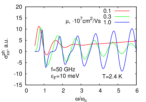
Figure 1: Dependency of the 2DEG photoconductivity upon the $\omega/\omega_{c}$ ratio. The microwave radiation frequency is 50 GHz.

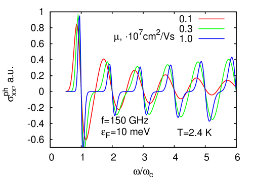
Figure 2: Dependency of the 2DEG photoconductivity upon the $\omega/\omega_{c}$ ratio. The microwave radiation frequency is 150 GHz.

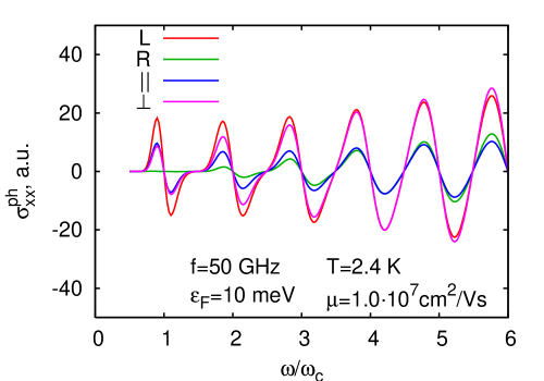
Figure 3: Dependency of the 2DEG photoconductivity upon the $\omega/\omega_{c}$ ratio for various polarizations of the microwave radiation: left circular (L), right circular (R), linear longitudinal with respect to the dc field ($||$), linear transverse with respect to the dc field ($\perp$).

References

• (1) M. A. Zudov and R. R. Du, L. N. Pfeiffer and K. W. West, arXiv:cond-mat/0210034; Phys. Rev. Lett. 90, 046807 (2003); EP2S-15, Nara, Japan. 2003
• (2) R. G. Mani, J. H. Smet, K. von Klitzing, V. Narayanamurti, W. B. Johnson, and V. Umansky, Nature, 420, 646 (2002); arXiv:cond-mat/0306388; 26-Inter. Conf. Phys. of Semicond. Edinburg. 2002; Ep2S-15, Nara, Japan. 2003
• (3) V. I. Ryzhii, Fizika Tverdogo Tela 11, 2078 (1970); V. I. Ryzhii, JETP Letters 7, 28 (1968)
• (4) Adam C. Durst, Subir Sachdev, N. Read, and S. M. Girvin, arXiv:cond-mat/0301569; EP2S-15, Nara, Japan. 2003. Phys. Rev. Lett. 91, 086903 (2003)
• (5) Junren Shi and X. C. Xie, arXiv:cond-mat/0302393, Phys. Rev. Lett. 91, 086801 (2003)
• (6) S. A. Mikhailov, arXiv:cond-mat/0303130
• (7) L. A. Dmitriev, M. G. Vavilov, I. L. Aleiner, A. D. Mirlin, D. G.Polyakov, arXiv:cond-mat/0310668
• (8) L. A. Dmitriev, A. D. Mirlin, D. G. Polyakov, arXiv:cond-mat/0304529
• (9) A. F. Volkov and V. V. Pavlovskii, arXiv:cond-mat/0305562; Phys. Rev. B 69, 125305 (2004)
• (10) M. G. Vavilov, I. L. Aleiner, arXiv:cond-mat/0305478, Phys. Rev. B 69, 035303 (2004)
• (11) A similar transformation was performed in: M. Torres, A. Kunold, cond-mat/0407468, Phys. Rev. B. 71, 115313 (2005)
• (12) V. P. Kalashnikov, Teoreticheskaya i Matematicheskaya Fizika 9, 94, (1971)
• (13) V. P. Kalashnikov, Teoreticheskaya i Matematicheskaya Fizika 34, 412, (1978)
Refer to caption