Subgap tunnelling through channels of polarons and bipolarons in chain conductors.

Abstract

We suggest a theory of internal coherent tunnelling in the pseudogap region where the applied voltage is below the free electron gap. We consider quasi 1D systems where the gap is originated by a lattice dimerization (Peierls or SSH effect) like in polyacethylene, as well as low symmetry 1D semiconductors. Results may be applied to several types of conjugated polymers, to semiconducting nanotubes and to quantum wires of semiconductors. The approach may be generalized to tunnelling in strongly correlated systems showing the pseudogap effect, like the family of High Tc materials in the undoped limit. We demonstrate the evolution of tunnelling current-voltage characteristics from smearing the free electron gap down to threshold for tunnelling of polarons and further down to the region of bi-electronic tunnelling via bipolarons or kink pairs. The interchain tunnelling is described in a parallel comparison with the on chain optical absorption, also within the subgap region.

I Introduction.

The interchain, interplane transport of electrons in low dimensional (quasi 1D, 2D) materials attracts much attention sigma-c in view of striking differences between longitudinal and transverse transport mechanisms revealing a general problematics of strongly correlated electronic systems. Beyond the low field (linear) conduction, the tunnelling current-voltage J-U characteristics $J(U)$, $\sigma=dJ/dU$ are of particular importance. The interest has been renewed thanks to recently developed latyshev design of intrinsic tunnelling devices where electronic transitions between weakly coupled chains or planes take place in the bulk of the unperturbed material.

The first feature one expects to see at any tunnelling experiment in gapful conductors is the regime of free electrons when the current onset corresponds to the voltage $U=E_{g}^{0}$ of the gap in the spectrum of electrons. But contrarily to usual systems, like semi- or even superconductors, there is also a possibility for tunnelling within the subgap region $E_{g}<U<E_{g}^{0}$. It is related to the pseudogap (PG) phenomenon known for strongly correlated electrons in general, well pronounces in quasi 1D systems and particularly in cases where the gap is opened by a spontaneous symmetry breaking (see mb:02 and refs. therein). The PG is originated by a difference, sometimes qualitative, between three forms of electronic states: a) short living excitations which are close to free electrons, b) dressed stationary excitations of the correlated systems, and c) added particles which modify the ground state itself PGdef . For our typical examples of electrons on a flexible lattice, the modification results in self-trapped states (b) like single particle $\nu=1$ polarons with energies $W_{1}<\Delta_{0}$ below the single electron (a) activation energy $\Delta_{0}$; then the new gap $E_{g}<E_{g}^{0}=2\Delta_{0}$ will be observed as a true threshold with the PG in between. There may be also contributions of two-particle $\nu=2$ states (c) - bipolarons, which energy gain per electron is larger than for polarons $W_{2}<2W_{1}$. While the cases (a,b) are common for low symmetry and discrete symmetry cases, for (c) there is a further drastic effect of a spontaneous symmetry breaking like the case of the polyacethylene $(CH)_{x}$ or of some doubly commensurate CDWs. Now the bipolarons are decoupled into particles with a nontrivial topology, solitons or kinks, changing the sign of the order parameter of the dimerization. The situation is further intricate in systems with a continuous GS degeneracy like Incommensurate Charge Density Waves (ICDW) or Wigner crystals. Here even the self-trapping of a single electron is allowed to lead to topologically nontrivial states, the amplitude solitons ASs. In the same class we find a more common case of acoustic polarons in a 1D semiconductor mb-ecrys ; bm:03 .

Properties of systems with different types of the GS degeneracy, and required theoretical approaches, are quite different. Here we shall concentrate on systems with a discrete, precisely double, degeneracy which also include most basic elements of non-degenerate systems. Theoretically, the tunnelling in CDWs was studied in details for regimes of free electrons free when the current onset corresponds to the voltage $U=E_{g}^{0}$ of the gap in the spectrum of electrons. We shall consider the tunnelling in the PG regime. We shall follow the method mb:02 developed for studies of single particle spectral density $I(p,\omega)$ in applications to PES and ARPES intensities. We refer to this publication for details in techniques and literature.

A word of notations. In the following we shall invoke many quantities with the dimension of energy (or frequency, since we shall keep $\hbar=1$) which will be classified according to different characters (with indices). $U>0$ and $\Omega>0$ will be the external voltage difference for tunnelling and the external frequency for PES or optics. $E>0$ will always stay for electronic eigenvalue in a given potential, negative values will be addressed explicitly as $-E$. $V_{\nu}(E)$ will be branches of a total energy (of deformations together with electronic energies) supporting eigenstates $\pm E$ which may be filled with occupation numbers $\nu=0,1,2$. $W_{\nu}$ will be total energies of stationary states, that is $W_{\nu}=\min_{E}V_{\nu}(E)=V_{\nu}(E_{\nu})$. $\omega_{0}\ll E$ will be the frequency of a collective mode (phonons specifically to CDWs) which interaction with electrons is responsible for their self-trapping. The collective deformation $\Delta(x)$ will also be measured as the potential energy experienced by electrons. We shall keep the electron charge $e=1$ hence potentials will be measured as energies and the interchain current $J$ will have the dimension number-of-particles/unit-time/unit-length. The indices $j=a,b$ will number coupled chains; indices $i$ will number moments $\tau_{i}$ of time for virtual processes.

II Spectroscopies of the pseudogap.

A possibility of tunnelling or of other excitations within the gap in spectra of free electrons $E<\Delta_{0}$ is related to a more general phenomenon of the pseudogap PG. For electrons, the PG signifies the remnants of the spectral density $I(\Omega,P)$, or the integrated one $I(\Omega)=\int I(\Omega,P)dP/2\pi$, at $W_{1}<\Omega<\Delta_{0}$ where $W_{1}$ is the absolute boundary of the spectrum. $W_{1}$ is the energy of a fully dressed state of one electron interacting with other degrees of freedom. (There may be totally external modes like deformations or polarizations for usual polarons, external modes essentially modified by the bath of electrons like in CDWs, internal collective modes of electronic system itself like in SDWs.) Most commonly, the self-trapped state of one electron is known as the ”polaron ” while more complex objects, solitons, can appear for systems with continuously degenerate GSs (see braz:84 for a review).

The functions $I(\Omega)$ and $I(\Omega,P)$ are measured directly in PES and ARPES experiments (these abbreviations stay for the integrated Photo-Emission Spectroscopy and for the Angle (that is momentum) Resolved one). As such they have been studied theoretically for the PG region by the present authors mb:02 ; mb-ecrys ; bm:03 and we refer to these publications for a more comprehensive discussion and for the literature review. The one electron spectra can be accessed also in traditional external tunnelling experiments: junctions or STM. For the last case, and practically for macroscopic point junctions, only the integrated $I(\Omega)$ is measured. Elements of the full dependence $I(\Omega,P)$ become necessary to describe strongly anisotropic materials (layered quasi-2D or chain quasi-1D ones) where the coherent tunnelling is realized in internal junctions of ”mesa” type devices latyshev . Here the tunnelling goes between adjacent layers within the single crystal of the same material, hence the momentum is preserved. In a simpler version, the internal subgap tunnelling takes place from free electrons of some metallic bands or pockets to polaronic states within gapful spectra which probably takes place in $NbSe_{3}$ latyshev+ . Otherwise it measures actually the joint spectral density for creation a particle-hole excitation at adjacent chains (the interchain exciton). In this respect it will be instructive to compare the coherent tunnelling and the subgap optical absorption OA (see a short excursion and references in mb:02 , III.E). A less expected version of the internal tunnelling is a possibility for bi-electronic transfers (tunnelling of bipolarons or of kink-antikink pairs) which usually is attributed only to superconductors. We shall see that these processes extend the PG further down to even lower voltages.

In any case, the tunnelling current $J(U)$ is given by the transition rate of electrons between two subsystems $a,b$ kept at the potential difference $U$. For a weak coupling $t_{\bot}$, the electron tunnelling from $a$ to $b$ is given by the convolution of spectral densities

$$J\sim t_{\bot}^{2}\int_{0}^{U}I_{a}(-\Omega,P)I_{b}(U-\Omega,P)\left|\Lambda(P)\right|^{2}d\Omega dP$$

if the momentum is conserved, or of their integrals $J\sim t_{\bot}^{2}\int_{0}^{U}I_{a}(-\Omega)I_{b}(U-\Omega)d\Omega$ for the incoherent tunnelling. (Everywhere we assume $T=0$.) Recall that for free electrons with a spectrum $E(P)$ we have $I(\Omega,P)\sim\delta(|\Omega|-E(P))$ while $I(\Omega)$ becomes the DOS $I(\Omega)\Rightarrow N(\Omega)$, e.g. for $D=1$ $I(\Omega)\sim t_{\bot}^{2}m^{1/2}(\Omega-\Delta_{0})^{-1/2}$ near the bottom of the free band where the electron effective mass is $m$.

Consider briefly the case where one of reservoirs, say $\#b$, is composed by free electrons with a known DOS $N_{b}(\Omega)$. One of applications of a tunnelling between the free spectrum and the PG may be the case of several families of conjugated polymers (polypyrolle, polythiophene) where origins of filled, $\pi$ or empty, $\pi^{\ast}$ bands below and above the gap are essentially different. Then the polaronic effect, hence the PG, may be pronounced only for one type of particles: electrons or holes. The same concerns 1D systems made of semiconducting wires where both effective masses and deformation potentials for electrons and holes are usually very different. Then, for the incoherent tunnelling, $I_{a}(U)$ gives directly either the tunnelling current $J(U)\sim I_{a}(U)$ (if $N_{b}$ has a sharp peak at the Fermi level, which is typical for using junctions with superconductors) or the tunnelling differential conductance $\sigma=dJ/dU\sim I_{a}(U)$ (if $N_{b}\approx const$ at the Fermi surface).

Below we shall be mostly interested in systems with the charge conjugated symmetry (or qualitatively equivalent ones); the examples are carbon nanotubes, symmetric conjugated polymers like polyphenylenes, polyanilines and polymers where the gap is formed (partly at least) by the spontaneous symmetry breaking: the polyacethylenes (polymers ). Numerical details will be presented for the last rich case. In all these cases the PG will exist near both rimes $\pm\Delta_{0}$ of the free excitation gap $E_{g}^{0}=2\Delta_{0}$.

Recall now some known results for $I(\Omega)$ within the PG mb:02 . It has the form $I=A\exp(-S)$ where the action $S=S(\Omega)$ is proportional to the big parameter of our adiabatic approximation: $S\sim\Delta_{0}/\omega_{0}\gg 1$. $S(\Omega)$ is determined by an optimal fluctuation localized in space and time (an instanton) which supports the necessary split-off local level $E$. In principle, the prefactor $A=A(\Omega)$ also depends on $\Omega$ and may show power law dependencies near extremals $0,W_{1}$. But within constraints of the adiabatic approximation $\delta\Omega\gg\omega_{0}$ the dependence $A(\Omega)$ is negligible in comparison with the one of $S(\Omega)$. The characteristic value of $A$ may be important for estimates of the overall magnitude of observable effects. Thus for the single particle integrated intensity $A\sim(\omega W_{1})^{-1/2}$ and $A_{P}\sim(m\Delta_{0}\omega W_{1})^{-1/2}$ for the momentum resolved intensity; here $m$ is the effective electron mass $m\sim\Delta_{0}/v_{F}^{2}$. Appendix B contains derivation of the prefactor specifically for the tunnelling processes.

In limiting cases we have mb:02

1. Near the entry to the PG, just below the free edge $\Delta_{0}$:

$$\Delta_{0}-W_{1}\gg\Delta_{0}-\Omega>0~{}:\ I=A\exp\left[-\frac{cnst}{\omega_{0}}\left(1-\frac{\Omega}{\Delta_{0}}\right)^{3/2}\right].$$ (1)

2. Near the low end of the PG, just above the true spectral boundary $W_{1}$:

$$\Delta_{0}-W_{1}\gg\Omega-W_{1}>0~{}:\ I=A\exp\left[-cnst\frac{\Delta_{0}-W_{1}}{\omega_{0}}-cnst\frac{\Omega-W_{1}}{\omega_{0}}\ln\left(\frac{\Omega-W_{1}}{\Delta_{0}-W_{1}}\right)\right].$$ (2)

The total dependence $I(\Omega)$ and the values of numerical constants in the above limiting laws, can be determined approximately mb:02 with the help of the instanton techniques simplified by the zero dimensional reduction (the Anzats of an effective particle which we shall recall and extend below). The resulting curve is plotted at the figure 1. Moreover, the regime (1.) can be mapped exactly mb:02 upon the problem of a particle in a quenched random uncorrelated potential which here is created by instantaneous quantum fluctuations of the media. The known exact solution halperin provides the reference value of the coefficient in the exponent of (1), from which our approximate value differs only by $8\%$ mb:02 .

Figure 1: The logarithmic plot for tunnelling or absorption intensities $\ln I\sim-S$ in the pseudogap regime: between $2W_{1}$ and $2\Delta_{0}$.

Figure 2: The logarithmic plot for bi-electron tunnelling or for optical absorption intensities $\ln I\sim-S$ in the two particle pseudogap regime: between $2W_{s}$ and $2\Delta_{0}$. Notice the $\sqrt{\Omega-2E_{s}}$ singularity near the two soliton threshold.

Recall for comparison the usual regime $U>E_{g}^{0}$ of the allowed tunnelling which is dominated by free electronic states. The current of the coherent tunnelling between chains $a,b$ is given as

$$J\sim t_{\perp}^{2}\int\frac{dp}{2\pi}\delta(E_{b}(p)-U-E_{a}(p))\left|\Lambda(p)\right|^{2},\quad\Lambda(p)=\int dx\Psi_{bp}(x)\Psi_{ap}^{\ast}(x)$$ (3)

with $E_{a,b}(p)\approx\pm\left(\Delta_{0}+p^{2}/2m_{e}\right)$ and $\Psi_{jp}(x)$ being the Bloch functions. It is instructive to compare the interchain tunnelling probability with the on chain interband optical absorption OA when the matrix element of density $\Lambda(p)$ changes to the one of the momentum: $t_{\bot}\Lambda(p)\Rightarrow\Lambda_{OA}(p)$. In both cases the $e-h$ pair is created and the same spectral densities are involved. The difference is in matrix elements: the OA takes place between states of opposite parity while the tunnelling requires for the same parity. The on-chain OA between edges $\pm\Delta_{0}$ of the free gap is known to be allowed since the parity of states near $\pm\Delta_{0}$ is opposite, hence $\Lambda_{OA}$ is finite and the OA intensity as a function of frequency $\Omega$ rises as $I_{OA}\propto 1/\sqrt{\Omega-2\Delta_{0}}$. But for the same reason, the tunnelling matrix element between identical chains is prohibited at $p=0$ and the tunnelling will show only a weak edge onset $J\sim\sqrt{\Omega-2\Delta_{0}}$. Nevertheless, in many cases of gaps opened due to spontaneous dimerization, the neighboring chains tend to order in antiphase. Now the shift by half a period permute states with $E\gtrless 0$ then the parity of states near opposite rims $\pm\Delta_{0}$ at neighboring chains is equal, the tunnelling becomes allowed and the usual singularity is restored: $J\propto 1/\sqrt{U-2\Delta_{0}}$.

Going down into the PG $\Omega<\Delta_{0}$, the above analysis applies to the on-chain optics but changes drastically for the interchain tunnelling. The tunnelling will be studied in details below, here we shall only mention in advance an effect of spatial incoherence of optimal quantum fluctuations at different chains which removes completely the constraints of orthogonality. The case of the on-chain OA can be analyzed briefly already here. The OA is given by the convolution of two fast decaying functions of the energy

$$I_{OA}\sim\int I(\Omega_{1},P)I(\Omega-\Omega_{1},P)\left|\Lambda_{OA}(P)\right|^{2}d\Omega_{1}dP$$

$$\int\exp\left[-S(\Omega_{1},P)-S(\Omega-\Omega_{1},P)\right]\left|\Lambda(\Omega_{1},\Omega_{1}-\Omega)\right|^{2}d\Omega_{1}\sim$$

$$\Lambda^{2}(\Omega/2,-\Omega/2)\left(S^{\prime\prime}\right)^{-1/2}\exp\left[-2S(\Omega/2)\right]=$$

$$\left(S^{\prime\prime}(\Omega/2)\right)^{-1/2}I^{2}(\Omega/2);\ S^{\prime\prime}=\frac{d^{2}S}{d\Omega^{2}}.$$ (4)

Here we have used that for the convex function $S(\Omega)$, as given by (1,2), the minimum of the expression $S(\Omega_{1},P)+S(\Omega-\Omega_{1},P)$ lies at the middle $\Omega_{1}=U/2$. At this point the electron levels $E$ and $E-\Omega$ are placed symmetrically, wave functions have opposite parity, hence $\Lambda(E,-E)\neq 0$ is finite. This is the case of typical Peierls insulators. But for systems where the basis wave functions of valent and conductive bands have the same parity (the dipole OA is not allowed), $\Lambda_{OA}(E,-E)=0$ and we have to consider in (4) the deviations from the symmetry condition. Now $\Lambda_{OA}(E_{a},E_{b})\sim(E_{a}+E_{b})^{2}$ and the saddle point integration in (4) gives another factor of $1/S^{\prime\prime}$ which is small as $\sim\omega_{0}/\Delta_{0}$. We arrive at the answer similar to (4) but with the small prefactor $\left(S^{\prime\prime}\right)^{-3/2}$.

Until now we did not consider the dependencies on the momentum $P$. In the full range of $\Omega$ and $P$, the spectral function $I(\Omega,P)$ has a rich structure which can be tested in the ARPES experiments. In observable quantities, the momentum dependence appears twice: via the matrix element $\Lambda(P)$ and via the action $S(\Omega)\Rightarrow S(\Omega,P)$. The analysis is simplified for the regime 2: the low polaron boundary $W_{1}$. Here the action dependence on $\Omega$ and $P$ comes through the single variable $\Omega\Rightarrow\Omega+P^{2}/2M_{1}$ where $M_{1}\sim m\Delta_{0}^{2}/\omega_{0}^{2}$, is a heavy mass of the polaron center motion. This kinetic energy contribution can be neglected in compare to the matrix element dependence on $P$ which confines $\Lambda^{2}\sim\left|\Psi_{P}\right|^{4}$ within the characteristic momenta distribution $|\Psi_{P}|^{2}$ of the wave function $\Psi(x)$ of the self-trapped electronic state localized over the scale $L\sim\xi_{0}$: beyond $P\sim\xi_{0}^{-1}=\Delta_{0}/\hbar v_{F}$, the function $\Lambda(P)$ falls off exponentially. (At this scale, the recoil kinetic energy $P^{2}/2M\sim\omega_{0}^{2}/\Delta_{0}$ is small in compare to the energy width $\epsilon\sim\left(S^{\prime\prime}\right)^{-1/2}\sim\left(\omega_{0}(W\,_{1}-\Omega)\right)^{1/2}\gg\omega_{0}$. Then the final integration over $P$ affects only $\Lambda(P)$ and gives a constant factor $\sim 1/\xi_{0}$.) Altogether we find for tunnelling just the law (2) with $\Omega\rightarrow U/2$.

In the regime 1., near the free edge, the states are shallow $\epsilon=1-E/\Delta_{0}<<1$ and extended $L/\xi_{0}\sim\epsilon^{-1/2}\gg 1$. The effective mass $M$ for the center of motion becomes light, energy dependent

$$M\sim\frac{\epsilon^{2}}{\omega_{0}^{2}L}\sim\frac{\epsilon^{5/2}}{\omega_{0}^{2}},$$

but the characteristic energy scale of the form factor $\sim M^{-1}L^{-2}\sim\omega_{0}^{2}\epsilon^{-3/2}$ is still small in comparison with the characteristic energy width $\sim\omega_{0}^{2/3}$ of (1). So again we integrate separately the factor $\int\Lambda^{2}(P)dP\sim\int dP\Psi_{P}^{4}\sim L$ to obtain an additional prefactor $\epsilon^{-1/2}$ for the tunnelling law (1) with $\Omega\rightarrow U/2$.

Recall that for the ARPES with independent variations of $\Omega$ and $P$, their interference may lead to rather unexpected and potentially observable phenomena (mb:02 , section III.D). One of them is the ”quasi spectrum”: the intensity maximum over the line $\Delta_{0}-\Omega\sim P^{1/2}$ within the PG $\Omega<\Delta_{0}$ (mb:02 , section III.D, case B1, Eq.49). Another effect is the emergence of instantons at high $P$ within the domain of free electron region $>\Omega>\Delta_{0}$ leading to the enhanced intensity within the band $0<\Omega-\Delta_{0}<cnst/P^{3}$ (mb:02 , section III.D, case B3, Eq.51).

III Tunnelling: the derivations.

We shall follow the adiabatic method of earlier publications mb:02 ; mb-ecrys ; bm:03 assuming a smallness of collective frequencies $\omega_{0}$ in compare with the electronic gap: $\omega_{0}\ll\Delta_{0}$. Now, electrons are moving in a slowly varying potential $\Delta(x,t)$, so that at any instance $t$ their energies $E_{j}(t)$ and wave functions $\Psi_{j}(x,t)$ are defined from a stationary Schrodinger equation $H\Psi(x,t)=E(t)\Psi(x,E(t))$ (Eq. (23) below will give an example). The Hamiltonian $H=H(x,\Delta(x,t))$ depends on the instantaneous configuration $\Delta(x,t)$ so that $E(t)$ and $\Psi(x,E(t))$ depend on time only parametrically. Exponentially small probabilities which we are studying here are determined by steepest descent paths in the joint space $[\Delta(x),t]$ of configurations and the time, that is by a proximity of the saddle point of the action $S$. It is commonly believed, in analogy with the usual WKB, that the saddle point, the extremum of $S$ over $\Delta$ and $t$, lie at the imaginary axis of $t$ so that, as usual, we shall assume $t\Rightarrow it$ and correspondingly $S\Rightarrow iS$ since now on.

Consider the system of two weakly coupled chains $j=a,b$ which are put at the electric potential difference $U$. The system is described by the total action

$$S_{ab}=S_{a}+S_{b}+t_{\perp}\int dxdt(\hat{\Psi}_{a}^{{\dagger}}(x,t)\hat{\Psi}_{b}(x,t)+\hat{\Psi}_{b}^{{\dagger}}(x,t)\hat{\Psi}_{a}(x,t)),$$ (5)

where $S_{j}=S[\Delta_{j}(x,t)]$ are single chain actions and the term $\sim t_{\bot}$ describes the interchain hybridization of electronic sates. $\hat{\Psi}_{j}(x)$ are operators of electronic states.
The average transverse current is given by the functional integral

$$J=\frac{\int D[\Delta_{j}(x,t)]~{}it_{\perp}(\hat{\Psi}_{a}^{{\dagger}}(x,t)\hat{\Psi}_{b}(x,t)-\hat{\Psi}_{b}^{{\dagger}}(x,t)\hat{\Psi}_{a}(x,t))\exp[-S_{ab}]}{\int dxD[\Delta_{j}(x,t)]\exp[-S_{ab}]}.$$ (6)

III.1 One electron tunnelling.

We consider first the processes originated by the transfer of one electron between the chains. They appear already in the first order of expansion of the exponent in (5) in powers of $t_{\perp}$, which contribution to the current (6) can be written as

$$J=Z_{0}^{-2}t_{\perp}^{2}\int D\left[\Delta_{j}(x,t)\right]\int d(x-y)\int d(\tau_{1}-\tau_{2})$$ (7)

$$[\Psi_{a}^{\ast}(x,\tau_{1})\Psi_{b}(x,\tau_{1})\Psi_{a}(y,\tau_{2})\Psi_{b}^{\ast}(y,\tau_{2})\exp(-S(\tau_{1}-\tau_{2},\Delta_{j}(x,t))),$$

where the normalizing factor $Z_{0}^{-2}$ is the denominator in (6) taken at $t_{\perp}=0$. Here the time dependent action $S(\tau_{1}-\tau_{2})$ describes (in imaginary time) the process of transferring one particle from the doubly occupied level $E_{a}<0$ of the chains $a$ to the unoccupied level $E_{b}>0$ of the chain $b$ at the time $\tau_{1}$ and the inverse process at the time $\tau_{2}$. We have

$$S(\tau_{1}-\tau_{2},\Delta_{j}(x,t)) = \left\{\int_{-\infty}^{\tau_{1}}+\int_{\tau_{2}}^{\infty}\right\}dt[L_{a}(0)+L_{b}(0)]+\int_{\tau_{1}}^{\tau_{2}}dt[(L_{a}(-1)+L_{b}(1)-U]$$ (8)

$$= \int_{-\infty}^{\infty}dt[L_{a}(0)+L_{b}(0)]+\int_{\tau_{1}}^{\tau_{2}}dt[(E_{b}+E_{a}-U],$$

where $L_{j}(\nu)=L([\Delta_{j}],\nu)$ are Lagrangians of the $j$-th chain with the number of electrons changed by $\nu$. They are given as a sum of the kinetic term and the potential $V_{\nu}$:

$$L_{j}(\nu)=\int dx\frac{(\partial_{t}\Delta)^{2}}{g^{2}\omega_{0}^{2}}+V_{\nu}[\Delta(x,t)]~{};\ V_{\nu}=V_{0}+|\nu|E.$$ (9)

Here the potential term $V_{\nu}$ contains the energy of deformations and the sum over electron energies in filled states $\alpha$ which include both the vacuum states and the split off ones:

$$V_{{}_{\nu}}[\Delta(x,t)]=\int dx\frac{\Delta^{2}}{2g^{2}}+\sum_{E_{\alpha}<E_{F}}E_{\alpha}[\Delta(x,t)]-W_{GS}$$ (10)

(here $g$ is the coupling constant). $V_{\nu}$ is counted with respect to the GS energy $W_{GS}$ so that in the non perturbed $\Delta\equiv\Delta_{0}$ state $V_{{}_{\nu}}=|\nu|\Delta_{0}$ (the particle, electron for $\nu>0$ or hole for $\nu<0$, added instantaneously to the non deformed GS is placed at the lowest allowed energy, the gap rim $\Delta_{0}$).

The exact extremal (saddle point) trajectory is defined by equations

$$\delta S/\delta\Delta_{j}(x,t)=0~{},\ \partial S/\partial\tau_{1}=\partial S/\partial\tau_{2}=0.$$ (11)

Actually the explicit calculation of the action requires for approximations. We shall follow a way mb:02 of the zero dimensional reduction which reduces the whole manyfold of functions $\Delta_{j}(x,t)$ to a particular class

$$\Delta_{j}(x,t)\Rightarrow\Delta_{E}(x-X_{j}(t),E_{j}(t)),\;S[\Delta_{j}(x,t)]\Rightarrow S[E_{j}(t),X_{j}(t)]$$ (12)

of a given function $\Delta_{E}$ of $x$ (relative to a time dependent center of mass coordinate $X_{j}(t)$). $\Delta(x)$ is parameterized by a conveniently chosen (see mb:02 for examples) parameter for which a universal and economic choice is the eigenvalue $E_{j}(t)$. The requirement for the manyfold $\Delta(x,E)$ is that it supports a pair of eigenvalues $\pm E$ split off inside the gap $(-\Delta_{0},\Delta_{0})$ which span the whole necessary interval. The last simplification is to assume, in the spirit of all approaches of optimal fluctuations disorder ; optimal , that the potential supports one and only one pair of localized eigenstates $\Psi(x,\pm E)$. Explicit formulas for the Peierls case are given in the Appendix A.

Recall that for the OA problem we deal with one chain characterized by one pair of functions $E(t)$ and $X(t)$. But for the interchain tunnelling, the functions $E_{j}(t)$ at chains $j=a,b$ are not obliged to be identical and also the wells may be centered around different points $X_{j}(t)$. Within such a parametrization the variational equation in (11) yields the equation of motion for $E(t)$

$$f(E_{j})\left(\frac{dE_{j}}{dt}\right)^{2}-V_{\nu}(E_{j})-|\nu|U+H_{\nu j}~{}=0~{},\ \ f(E)=\frac{1}{g^{2}\omega_{0}^{2}}\int dx\left(\frac{\partial\Delta(x,E)}{\partial E}\right)^{2},$$ (13)

where $H_{\nu j}=cnst$ are the Hamiltonians which must be constants within each interval of integration in (8). Apparently, at the outer intervals $(t<\tau_{1})$,$(\tau_{2}<t)$ $H_{0j}=0$ to provide the return to the GS with $V_{0}=0$ at $t\rightarrow\pm\infty$. At the inner interval $(\tau_{1}<t<\tau_{2})$ $H_{1j}=E_{j}(\tau_{1})+U=E_{j}(\tau_{2})+U$ to preserve the continuity of velocities $\dot{E}_{j}$ at $t=\tau_{1,2}$. Since the values $E_{j}(\tau_{1,2})$ are determined uniquely by the equation of motion at the outer intervals, then $E_{j}(\tau_{1,2})$ coincide for both $j=a,b$, hence $H_{a}=H_{b}$ and the functions $E_{j}(t)$ become identical at any time $E_{a}(t)\equiv E_{b}(t)\equiv E(t)$. (Still, the shapes are allowed to be shifted by different centers $X_{j}(t)$: $\Delta_{a}(x-X_{a},t)\equiv\Delta_{b}(x-X_{b},t)$). Finally the extremal conditions (11) with respect to impact times $\tau_{i}$ in (8) yield

$$\left.E_{a}(t)+E_{b}(t)\right|_{t=\tau_{1,2}}=U~{}~{}\mathrm{hence}~{}~{}E_{a}(\tau_{1,2})=E_{b}(\tau_{1,2})=U/2.$$

The action is finite $S<\infty$, hence the transition probability is not zero, only for a closed trajectory, that is at presence of a turning point (as examples, see figures 5,6,7,8 in the Appendix A). There must be a minimal value of $E=E_{m}$ where $\dot{E}=0$ hence $V_{1}(E_{m})=U/2$ and $E_{m}<U/2$. The last condition requires for $minV_{1}(E)=W_{1}\leq U/2$ that is for $U>2W_{1}$ which determines the threshold voltage at twice the polaron energy.

We arrive at the effective one chain problem with the doubled effective action. The extremal tunnelling action is $S_{tun}=2S_{I}$ which is twice the exponent appearing in the spectral density $I$ with limiting laws (1,2). The full expression is

$$S_{tun}(U)=8\int_{E_{m}}^{U/2}dE\sqrt{f(V_{1}-U/2)}+8\int_{U/2}^{\Delta_{0}}dE\sqrt{fV_{0}}~{};\ V_{1}(E_{m})=U.$$ (14)

We obtain a final expression for the current after integration over $\Delta_{j}(x,t)$ around the extremal taking into account the zero modes related with translations of the instanton centers positions $X_{j}(t)$. (Details of calculations are given in the Appendix B)

$$J(U)\propto t_{\perp}^{2}M_{U}\omega_{0}\sqrt{\frac{dT}{dU}}\int\frac{dp}{2\pi}e^{-p^{2}l^{2}/4}\left|\Psi_{p}(U/2)\Psi_{p}(-U/2)\right|^{2}\exp[-2S_{I}(U/2)],$$ (15)

where $\Psi_{p}$ is the Fourier transforms of the wave functions $\Psi(x)$, the time $T$ is defined as $T=\int_{U/2}^{E_{m}}dE/\dot{E}$. The mean fluctuational displacement $l$ of the center of mass between the impact moments is given as

$$l^{2}=\int_{\tau_{1}}^{\tau_{2}}\frac{dt}{M(E(t))}=2\int_{E_{m}}^{U/2}\frac{dE}{M(E)}\frac{\sqrt{f(E)}}{\sqrt{V_{1}(E)-U/2}},$$

where $M(E)$ is the translational mass:

$$M(E)=\frac{2}{g^{2}\omega_{0}^{2}}\int dx\left(\frac{\partial\Delta(x,E)}{\partial x}\right)^{2}~{},\ M_{U}=M(U/2).$$ (16)

Note that the prefactor in Eq. (15), which is the matrix element between orthogonal states $\Psi(E)$ and $\Psi(-E)$, is always nonzero due to the integration over zero modes $X_{j}(t)$ (in contrast to results for the rigid lattice where it obeys the selection rules); see more in the Appendix B.

Comparing with the PES intensity $I(\Omega)$ calculated in mb:02 we see that, up to pre-exponential factors, the tunnelling current is proportional to the square of the PES intensity $I$: $J\propto t_{\perp}^{2}I^{2}(\Omega=U/2)$. E.g. near the threshold $U=2W_{1}$ we can write

$$J\sim\frac{t_{\perp}^{2}}{\Delta_{0}\xi_{0}}\left(\frac{\Delta_{0}}{\omega_{0}}\right)^{3/2}\exp\left[-C_{1}\frac{\Delta_{0}}{g\omega_{0}}\right]\exp\left[C_{2}\frac{(U-2W_{1})}{g\omega_{0}}\log\frac{2C_{3}\Delta_{0}}{(U-2W_{1})}\right].$$ (17)

The coefficients $C_{i}\sim 1$ can be found numerically from (14) as (for the Peierls model) $C_{1}=0.4$, $C_{2}=2.9$, $C_{3}=0.1$. (These values differ from the corresponding ones in mb:02 because of different normalizations of frequency $\omega_{0}$ in compare to $\omega_{ph}$).

III.2 Bi-electronic tunnelling.

It is known that the joint self-trapping of two electrons allows to further gain the energy resulting in stable states different from independent polarons. In general nondegenerate systems this is the bipolaron, confined within the length scale twice smaller than that of the polaron, the energy gain of the bound state $\delta E=\Delta_{0}-E$ is four times that of the polaron and the total energy gain of the bipolaron $\delta W_{2}=2\Delta_{0}-W_{2}$ is also four times that of two polarons. (Certainly these results neglect the energy loss due to the Coulomb repulsion which may become critical for the stability of a shallow bipolaron.) The same time, the total energy of one bipolaron $W_{2}=2\Delta_{0}-\delta W_{2}$ is larger than the energy of one polaron $W_{1}=\Delta_{0}-\delta W_{1}$ and even than the free electron energy $\Delta_{0}$. This is why bipolarons cannot be seen as thermal excitations while they are favored in case of doping. The information on their existence comes from the ground state of doped systems where bipolarons are recognized by their spinless character and special optical features (see bipol-polym for experimental examples on conducting polymers and bipol-th for relevant theoretical models). An important advantage of tunnelling experiments is a possibility to see bipolarons directly, at voltages $U$ below the two-polaron threshold $2W_{1}$ that is within the true single particle gap. This possibility comes from the fact that, for bipolarons as particles with the double charge $2e$, the voltage gain by transferring from one chain to another is $2U$, hence the threshold will be at $U=W_{2}<2W_{1}$. The probability of the bi-electron tunnelling is small as it appears only in the higher order $\sim t_{\perp}^{4}$ in interchain coupling. But it can be seen as extending below the one-electron threshold where no other excitations can contribute to the tunnelling current.

The bi-electronic contribution to the current can be written, by expanding (5) and (6), as

$$J_{2} = Z_{0}^{-2}t_{\perp}^{4}\int D[\Delta_{a}]D[\Delta_{b}]\int\prod_{i=1}^{3}dy_{i}d\tau_{i}\exp\left(-S(\tau_{i})\right)$$

$$\left[\Psi_{a}^{\ast}(x,\tau)\Psi_{b}(x,\tau)\Psi_{a}^{\ast}(y_{1},\tau_{1})\Psi_{b}(y_{1},\tau_{1})\Psi_{b}^{\ast}(y_{b},\tau_{2})\Psi_{a}(y_{2},\tau_{2})\Psi_{b}^{\ast}(y_{3},\tau_{3})\Psi_{a}(y_{3},\tau_{3})-\{2\leftrightarrow 3\}\right],$$

which generalizes expressions (7) and (8) for the one electron tunnelling. Here

$$S(\{\tau_{i}\}) = \left\{\int_{-\infty}^{\tau}+\int_{\tau_{3}}^{\infty}\right\}dt[L_{a}(0)+L_{b}(0)]+$$ (18)

$$\left\{\int_{\tau}^{\tau_{1}}+\int_{\tau_{2}}^{\tau_{3}}\right\}dt[(L_{a}(1)+L_{b}(1)-U]+\int_{\tau_{1}}^{\tau_{2}}dt[L_{a}(2)+L_{b}(2)-2U].$$

Within our model (9,10) the potentials $V$ are additive in energy $E$, then the action can be simplified as

$$S(\{\tau_{i}\})=2\int_{-\infty}^{\infty}dtL_{a}(0,t)+$$

$$\left\{\int_{\tau}^{\tau_{1}}+\int_{\tau_{2}}^{\tau_{3}}\right\}dt(E_{a}(t)+E_{b}(t)-U)+2\int_{\tau_{1}}^{\tau_{2}}dt(E_{a}(t)+E_{b}(t)-U).$$ (19)

The extremal solution is defined, as above, by equations of the type (11) but with four impact times $\tau_{i}$ instead of two. (Actually, in view of the time reversion symmetry, the number of boundary conditions is twice smaller.) A similar analysis of the extremal solution shows that optimal fluctuations $\Delta_{j}(x,t)$ are identical in shape, up to shifts of their centra: $X_{j}(t)$, $\Delta_{j}(x,t)\equiv\Delta(x-X_{j},t)$. Hence the energies are identical $E_{a}(t)\equiv E_{b}(t)$, and also the resonance conditions $2E(\tau_{i})=U$ take place at the impact moments $\tau_{i}$. Moreover, the simple hierarchy of our model $V_{2}-V_{1}\equiv V_{1}-V_{0}\equiv E-U/2$ shows that all branches $V_{\nu}(E)$ cross at the same point $E=U/2$ (see figures 5,6,7 below). Then the evolution $E(t)$ switches directly from the branch $\nu=0$ to the branch $\nu=2$ and back, without following the intermediate branch $\nu=1$. It means that the intervals $(\tau,\tau_{1})$ and $\,(\tau_{2},\tau_{3})$ of one-electron transfers $\nu=1$ are confined to zero: $\tau=\tau_{1},\,\tau_{2}=\tau_{3}$. In other words, only processes of simultaneous tunnelling of pairs of particles are left. Notice that this picture changes in more general models, particularly taking into account important Coulomb interactions. They add, to the energy branch of a shallow bipolaron, the energy $\delta V_{2}\sim(e^{2}/\epsilon_{\bot}L)\ln(L/a_{\bot})$ where $\epsilon_{\bot}$ is the dielectric susceptibility of the media in the interchain direction, $L=L(E)$ is the localization length of $\Psi(x,E)$, such that $E\sim 1/(mL^{2})$. Now the intermediate intervals $(\tau=\tau_{1})$,$(\,\tau_{2}=\tau_{3})$ appear where the evolution follows the $\nu=1$ branches, see figure 8. With increasing Coulomb interactions this single particle interval becomes more pronounced and the bipolaronic threshold is shifted towards the one of two independent polarons.

In any case, the extremum solution for the action (18) is achieved on the instanton trajectory given be the equation

$$f(E)\dot{E}^{2}=V_{U}(E)=\min\{V_{0}(E),V_{1}(E)-U/2,V_{2}(E)-U\}.$$

The extremal action is

$$S_{2}(U)=8\int_{E_{m}}^{\Delta_{0}}dE\sqrt{f(E)V_{U}(E)}~{};\ V_{U}(E_{m})=V_{2}(E_{m})-U=0.$$ (20)

This action is finite if the turning point $E_{m}$ does exist, that is if $U\geq\min V_{2}=W_{2}$.

Notice that, neglecting Coulomb interactions, the energy $V_{\nu}$ is determined only by the total number $\nu=\nu_{e}+\nu_{h}=\nu(E)+(2-\nu(-E))$ of electrons and holes. Then the energy of the bipolaron (both $\nu(E)$ and $\nu(-E)$ are either empty or doubly occupied) and the energy of the exciton (both $\nu(E)=1$ and $\nu(-E)=1$ are singly occupied) are the same. Then the trajectory of the bi-electronic tunnelling becomes the same as the one for the case of optical absorption mb:02 , only the action is doubled $S_{2}(U)=2S_{OA}(\Omega=U)$. Up to the pre-exponential factor we have

$$J_{2}\propto t_{\perp}^{4}[I_{OA}(\Omega=U)]^{2},$$ (21)

where $I_{OA}(\Omega)$ is the optical absorption probability for one chain.

For common systems with a nondegenerate ground state, the dependence $S_{2}(U)$ resembles qualitatively the law 17 for the one-electron contribution, with a similar behavior near the threshold $U-2W_{1}\rightarrow U-W_{2}$. The situation changes for a doubly degenerate ground state where the bipolaron dissolves into a diverging pair of solitons (dimerization kinks). Thus for the Peierls model the evaluation of (20) gives, similar to the OA law of mb:02 , near the two particle threshold

$$J_{2}\sim t_{\perp}^{4}\exp\left(-\max S_{2}+\frac{4}{g\omega_{0}}\sqrt{6\Delta_{0}(U-2W_{s})}\right)~{};\ \max S_{2}=C_{4}\Delta_{0}/g\omega_{0}$$ (22)

with $C_{4}=3.77$. The overall dependence for the $\log J_{2}(U)\sim-S_{2}(U)$ is shown at the figure 2. Here we see explicitly that in the order $\sim t_{\perp}^{4}$ the threshold voltage $U=2W_{s}$ is smaller than $U=2W_{p}$ obtained in the order $\sim t_{\perp}^{2}$. Therefore this is the main contribution to the current in the region $2W_{s}<U<2W_{p}$. Figure 2 shows that the dependence of $J_{2}(U)$ near the low $U$ onset is much sharper than that of $J(U)$ at the figure 1 near the polaronic onset which corresponds to the higher singularity in the limiting formula (22) in compare to (17).

IV Discussion and Conclusions.

In quasi 1D systems with a gapful electronic spectrum, the interchain tunnelling (as well as PES or OA) can be used to test virtual electronic states within the pseudogap. Due to the interaction of electrons with a low frequency mode, phonons in our examples, the tunnelling is allowed in the subgap region $U<E_{g}^{0}$ which forms the pseudogap. The one electron processes lead to universal results similar both for systems with the build-in gap and for those where the gap is due to the spontaneous breaking of a discrete symmetry. The PG is entered with the law (1) and continues down to the threshold $U_{1}=2W_{1}$, approached with the law (2). This threshold corresponds to the interchain transfer of fully dressed particles: polarons with the energies $W_{1}$. But in tunnelling the PG is stretched even further down thanks to processes of a simultaneous tunnelling of two electrons. It terminates at the lower threshold $U_{2}=W_{2}$ or $U_{2}=2W_{s}$, $U_{2}<U_{1}$. Here $W_{2}$ is the energy of the bipolaron - a bound state of two electrons selftrapped together. In degenerate systems the bipolaron dissolves into unbound solitons, hence the threshold at $2W_{s}$ with a more pronounced dependence of the tunnelling rate (22) as well of the OA. Numerical results are presented at figures 1,2.

There is an important difference between subgap processes and the usual overgap transitions at $U,\Omega>E_{g}^{0}$ of free electrons in a rigid system. It comes, beyond intensities, from different character of matrix elements. Actually within the PG region there are no particular selection rules since the wave functions of virtual electronic states split off within the gap are localized having a broad distribution of momenta. Then the PG absorption is allowed independent on the interchain ordering. Contrarily, the regular tunnelling across the free gap shows an expected DOS singularity $\sim(E-E_{g}^{0})^{-1/2}$ for the out of phase interchain order while for the in-phase order the threshold is smooth $\sim(E-E_{g}^{0})^{1/2}$. This difference may be important to choose an experimental system adequate for studies of PGs. The smearing of the free edge singularity is a natural criterium for existence of the PG below it Kim:93 . But the total absence of this strong feature in systems with forbidden overgap transitions can allow for a better resolution of the whole PG region, down to the absolute threshold. Probably a very smooth manifestation of gaps in usual tunnelling experiments on CDWs tunneling , while the gaps show up clearly through activation laws, is related to this smooth crossover from the overgap to the subgap region. (Notice that the existing experiments refer mostly to ICDWs which, with their continuous degeneracy of the GS, must be studied specially which is beyond the scope of this article.)

Finally we shall discuss relations with other theoretical approaches. Most theories of tunnelling, see free , keep the following assumptions: i. They refer to the overgap region where interactions or fluctuations are not important and usually are not taken into account. ii. They refer to the incoherent tunnelling, local in space, which is a usual circumstance of traditional experiments. The PG in tunnelling was considered by Monz et al in free in the framework of the approach sadovskii . This method became popular recently in theories of the PG thanks to its easy implementation: it is sufficient to average results for a rigid system over a certain distribution of the gap values. Apparently this is the way to describe an average over a set of measurements performed on similar systems with various values of the gap, e.g. manipulating with the temperature, the pressure or a composition. But actually, as we could see above, the PG is formed by fluctuations localized both in space and time, the instantons, with localization parameters depend on the energy deficit being tested. There is an intermediate approach applied ohio to a complex of the PG phenomenon from optics to conductivity and susceptibility. It treats fluctuations as an instantaneous disorder due to quantum zero point fluctuations of the gap. Indeed, this picture can be well applied, as it was done already in brazov:76 , but only to dynamical processes and only in the upper PG region, just below the free gap $E_{g}^{0}$, which leads to the law (1). But deeper within the PG, the fluctuations are not instantaneous: they require for an increasingly longer time and become self-consistent with the measured electronic state leading to another law and to appearance of the lower threshold. Generalizations and deeper analysis of the model of the instantaneous disorder lead to interesting theoretical studies monien , but their applicability is very limited unless the variable time scale is realized as we have demonstrated in this and preceding articles.

Our approach can be compared to the work maki on the fluctuational creation of pairs of phase solitons in a 1D commensurate CDW under the longitudinal electric field. But in our case me deal, in effect, with the interchain tunnelling of pairs of solitons under the transverse field; also the solitons have a more complex character of a multielectronic origin.

In conclusion, the presented and earlier mb:02 ; bm:03 ; mb-ecrys studies recall for the necessity of realizing the variable time scale of subgap processes both in theory and in diverse interpretations of different groups of experiments (dynamic, kinetic, thermodynamic) which address excitations with very different life times.

Appendix A Details on self-trapping branches.

We consider the system of weakly coupled dimerised chains. Each chain is described by a usual electron-phonon Hamiltonian (Peierls, SSH models). Electron levels $E$ and wave functions $\Psi=\Psi(x,E)$ are determined by equations

$$[-v_{F}i\partial_{x}\sigma_{3}+\Delta(x)\sigma_{1}]\mathbf{\Psi}=E\mathbf{\Psi},$$ (23)

where $\sigma_{1,3}$ are the Pauli matrices, $\mathbf{\Psi}=(\Psi_{+},\Psi_{-})$, $\Psi_{\pm}(x)$ are the components of electron wave functions near Fermi points $\pm p_{F}$, and the real function $\Delta(x)$ is the amplitude of the alternating dimerization potential. The ground state of each chain is the Peierls dielectric with the gap $2\Delta_{0}$. The electron spectrum has the form $E_{p}^{2}=v_{F}^{2}p^{2}+\Delta_{0}^{2}$ (in the following we shall put the Fermi velocity $v_{F}=1$, $\Delta_{0}=1$ and, as everywhere, the Plank constant $\hbar=1$). The excited states are solitons (kinks), polarons and bi-solitons (kink-antikink pairs) which are characterized by electron levels localized deeply within the gap (see the review braz:84 ). The one parametric family of configurations $\Delta(x,E)$ supporting the single split-off pair of levels $\pm E$ can be written as

$$\Delta(x,E)=1-\frac{2\left(1-E^{2}\right)}{1+E\cosh\left(2x\left(1-E^{2}\right)^{1/2}\right)}$$ (24)

evolving from a shallow potential well at $E\approx 1$ through the stationary configuration for a polaron $\nu=1$ to the pair of diverging kinks at $E\rightarrow 0$ as shown at the figure 3. The potentials $V_{\nu}$ (for the $E$ level filling $\nu$) as functions of $E$ are given as

$$V_{\nu}(E)=\nu E+\frac{4}{\pi}\sqrt{1-E^{2}}-\frac{4}{\pi}E\cos^{-1}E.$$ (25)

The translational mass can be found as

$$M(E)=\frac{8\Delta_{0}^{3}}{g^{2}\omega_{0}^{2}}\left[\frac{1}{3}\tan^{3}\left(\cosh^{-1}\frac{1}{E}\right)-E^{2}\cosh^{-1}\frac{1}{E}+E^{2}\sqrt{1-E^{2}}\right].$$ (26)

Consider the matrix element between levels $\pm E$ in the Peierls state. The wave function has two components $(u,w)$ according to $\Psi=\Psi(x,E)=u\cos p_{F}x+w\sin p_{F}x$. Explicit expressions for split-off states are $u,w\sim\sqrt{1-\Delta{}^{2}\pm\partial_{x}\Delta}$. The equation for the bound eigenstate (23) shows the following symmetry: $w(x,E)=u(-x,E)$, $w(x,-E)=u(x,E)$, $u(x,-E)=-u(-x,E)$. Then $\Psi(x,E)=((u(x),u(-x))$, $\Psi(x,-E)=(-u(-x),u(x))$, with $u=u(x,E)$, which demonstrates explicitly the orthogonality of $\Psi(x,E)$ and $\Psi(x,-E)$. The matrix element in Eq. (15) becomes $\Lambda_{p}^{2}\sim\left|\Psi_{p}(E)\Psi_{p}(-E)\right|^{2}=\left|-u_{p}u_{-p}+u_{p}u_{p}\right|^{2}$. At $p=0$, $\Lambda=\Lambda_{0}=0$, hence for identical chains the transition at the free gap $\Omega=2\Delta_{0}$ is forbidden which removes the singularity at the gap threshold in a rigid system. But the true threshold at $2W_{1}$ for the subgap absorption or tunnelling are not subjected to this selection rule since the wave functions of localized states associated to the optimal fluctuation are distributed over the momentum region $p\sim\xi_{0}^{-1}$.

Figure 3 shows exact shapes $\Delta(x,E)$ of the equilibrium polaron (upper thick line) and of a well formed $(E=0.01)$ pair of solitons (lower thick line). Thin lines show exact shapes of optimal fluctuations necessary to create these states by tunnelling. Notice the much less pronounced shapes for optimal fluctuations in compare to the final states which facilitates the tunnelling.

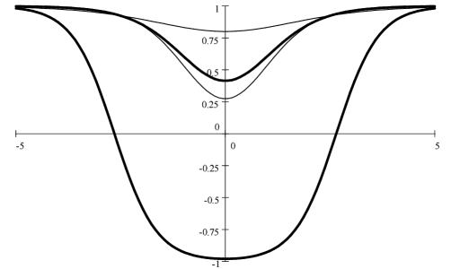
Figure 3: Exact shapes $\Delta(x,E)$ of the equilibrium polaron, $E=2^{-1/2}$ (upper thick line) and of a nearly formed ($E=0.01$) pare of solitons (lower thick line). Thin lines show exact shapes of optimal fluctuations necessary to create these states by tunnelling.

Figure 4 plots the total energy $V_{1}(E)$ of the single particle branch as a function of the associated energy of the bound state. $E=1$, $V_{1}(1)=1$ corresponds to the particle added to the unperturbed ground state, at the bottom of the continuous spectrum. $E=0$ is the mid-gap state reached for the limit of two divergent solitons when the total energy approaches the maximal value $V_{1}(0)=2W_{s}=4/\pi\approx 1.27$. In between, at $E_{1}=2^{-1/2}\approx 0.7$, $V_{1}(2^{-1/2})=W_{1}=2^{3/2}/\pi\approx 0.9$, the minimum corresponds to the stationary polaronic state. The short thin vertical line between plots $E$ and $V_{1}(E)$ points to the configuration (upper thin curve at the figure 3) of the fluctuation necessary for tunnelling to the polaron (the minimum of $V_{1}(E)$, upper thick curve at the figure 3).

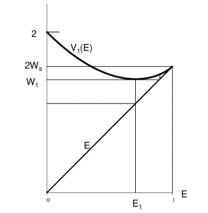
Figure 4: Total energy of the single particle branch $V_{1}(E)$ as a function of the energy $E$ of the associated bound state.

Next three figures plot the total energies $V_{\nu}-\nu U$ for different branches as a function of the energy $E$ of the associated bound state (all in units of $\Delta_{0}$). Branches are distinguished by their ordering at $E=1$. Figure 5 corresponds to the potential $U=1.2$ which is below the bi-electronic threshold; no branch is crossing $V=0$ axis, hence no final action is allowed and the current is zero.

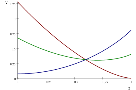
Figure 5: Total energies $V_{\nu}-\nu U$ for different tunnelling branches $V_{\nu}-\nu U$ as a function of the energy $E$ of the associated bound state. This figure corresponds to $U=1.2$ which is below the bi-electronic threshold.

Figure 6 corresponds to the potential $U=1.4$ which is between the bi-electronic threshold $2W_{s}=4/\pi\approx 1.3$ and the polaronic one $2W_{1}=1.8$; the bi-electronic branch crosses the axis $V=0$ at the point $E_{m}$, the action is finite, hence a nonzero tunnelling of two electrons is allowed.

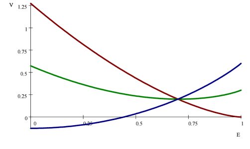
Figure 6: Tunnelling branches $V_{\nu}-\nu U$ as a function of the energy $E$ of the associated bound state. This figure corresponds to $U=1.4$ which is between the thresholds for tunnelling of bipolarons and polarons.

Figure 7 corresponds to the potential $U=1.8$, above the bi-electronic threshold $2W_{s}=4/\pi\approx 1.3$, exactly at the polaronic one $2W_{1}=1.8$. Now two parallel processes of one- and two- electron tunnelling are allowed.

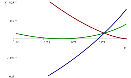
Figure 7: Tunnelling branches $V_{\nu}-\nu U$ as a function of the energy $E$ of the associated bound state (over a selected interval). This figure corresponds to $U=1.8$ which is just at the polaronic threshold, above the bipolaronic one.

The figure 8 corresponds to the potential $U=1.6$ between the bi-electronic threshold $2W_{s}=4/\pi\approx 1.3$, and the polaronic one $2W_{1}=1.8$. Contrary to the figure 6, the Coulomb interaction is taken into account which lifts the degeneracy of the earlier crossing point of three branches. The one electron term $\nu=1$ does not cross $V=0$ axis yet, but it passes below two other terms in a vicinity of their crossing. Now the optimal bi-electronic tunnelling takes place via a sequence of two single electronic processes confined in time.

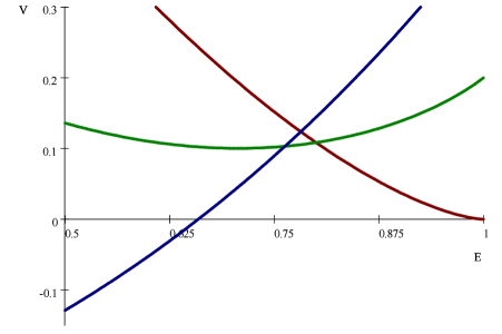
Figure 8: Tunnelling branches $V_{\nu}-\nu U$ as a function of the energy $E$ of the associated bound state. This figure corresponds to $U=1.6$ which is between the thresholds for tunnelling of bipolarons and polarons. Contrarily to the figure 6, the Coulomb interaction is taken into account which lifts the crossing degeneracy.

Appendix B Derivation of prefactor

We need to perform the integration over $\Delta_{j}(x,t)$ around the extremal taking into account the zero modes related to translations of positions $X_{j}(t)$ of the instanton centers. The path integration over the gapless mode $X(t)$ is important, particularly for the matrix element: the overlap of wave functions evolves following $X_{a}(t)-X_{b}(t)$ while their localization follows the evolution of $E(t)$. We shall work within the zero dimensional reduction of Eq.(12).

We expand the field $\Delta_{j}(x,t)$ in the vicinity of the instanton solution as

$$\Delta_{j}(x,t)=\Delta_{0}(x-X_{j}(t),E_{j}(t)+\delta(x-X_{j}(t),t)).$$ (27)

Following mb:02 , we rewrite (III.1) as

$$J\propto t_{\perp}^{2}\prod_{j=a,b}\int d(x-y)d(\tau_{1}-\tau_{2})\int D[E_{j}]D[X_{j}]J_{X_{j}}J_{E_{j}}\exp(-S)$$

$$\Psi_{a}^{\ast}(x-X_{a}(\tau_{1}),E(\tau_{1}))\Psi_{a}(y-X_{a}(\tau_{2}),E(\tau_{2}))\Psi_{b}(x-X_{b}(\tau_{1}),-E(\tau_{1}))\Psi_{b}^{\ast}(y-X_{b}(\tau_{2}),-E(\tau_{2})),$$ (28)

where $J_{X}=\propto\prod_{n=1}^{N}\sqrt{M(E(t_{n}))}$, $J_{E_{j}}\propto\prod_{n=1}^{N}\sqrt{f(E_{j}(t_{n}))}$ are the Jacobians of the transformation (12). ($N\rightarrow\infty$ is the number of points for the intermediate discretization of the time axis.) We integrate over the zero mode $X(t)$ and take into account fluctuations of the instanton shape due to variations of the parameter $E_{0}(t)$.

The action in (12) has the form

$$S[X,E]=\sum_{j=a,b}dt\left(M(E_{j}(t))\dot{X_{j}}^{2}/2+f(E_{j})\dot{E}_{j}^{2}/2+{V}_{U}(E_{j})\right)$$

with $V_{U}(E)$ from (20). The integration over $DX_{i}(t)$ is carried out exactly after the transformation $M\dot{X}^{2}=\dot{Z}^{2}$ using the known expression

$$\int D[x]\exp\left(-\int_{t_{1}}^{t_{2}}dt(\frac{\dot{x}^{2}}{2}+V(x))\right)\sim\exp(-S_{cl})\sqrt{\frac{d^{2}S_{cl}}{dx_{1}dx_{2}}},$$ (29)

where $x_{1}=x(t_{1})$, $x_{2}=x(t_{2})$. Next, we perform in (28) the remnant integrations over coordinates at the impact moments: $X_{1}=X_{a}(\tau_{1})$, $X_{2}=X_{a}(\tau_{2})$, $Y_{1}=X_{b}(\tau_{1})$, $Y_{2}=X_{b}(\tau_{2})$:

$$J\propto t_{\perp}^{2}\int dxd\tau_{1}dX_{1}dX_{2}e^{-\frac{(X_{1}-X_{2})^{2}}{l^{2}}}\Psi_{a}^{\ast}(x-X_{1},E(t_{1}))\Psi_{a}(y-X_{2},E(t_{2}))\frac{\sqrt{M_{1}}}{l_{1}}$$

$$dY_{1}dY_{2}e^{-\frac{(Y_{1}-Y_{2})^{2}}{l^{2}}}\Psi_{b}^{\ast}(x-Y_{1},-E(t_{1}))\Psi_{b}(y-Y_{2},-E(t_{2}))\frac{\sqrt{M_{2}}}{l_{2}}\exp[-S_{E}(E)].$$ (30)

Here $M_{i}=M_{i}(\tau_{1,2})$, and the same for $l_{i}$, are functions of energies in these points which finally become $E_{i}=E_{i}(\tau_{1,2})=U/2$. Using Fourier transforms, we rewrite the product of wave functions as

$$\int dpdqd\tilde{p}d\tilde{q}\Psi_{a,p}^{\ast}e^{-ip(x-X_{1})}\Psi_{a,q}e^{iq(y-X_{2})}\Psi_{b,\tilde{p}}e^{i\tilde{p}(x-Y_{1})}\Psi_{b,\tilde{q}}e^{-i\tilde{q}(y-Y_{2})}.$$

Integration over $dxdy$ gives $\delta(p-\tilde{p})$, $\delta(q-\tilde{q})$ and integration over $dX_{2},dY_{2}$ gives $L\delta(p-q)$. After integration over $d(X_{1}-X_{2})d(Y_{1}-Y_{2})$ we arrive at the result (15). The factor $\sqrt{{dT}/{dU}}=1/\sqrt{d^{2}S/dT^{2}}$ in (15) after integration over $D[E_{i}(t)]$ which was performed using again the equation (29).

References

- (1) P. W. Anderson, Science 279,1196(1998); M. Turlakov, A.J. Leggett, Phys. Rev. B 63, 064518 (2001) and rfs. therein.
- (2) Yu. I. Latyshev, A. A. Sinchenko, L. N. Bulaevskii, V.N. Pavlenko, P. Monceau, JETP Letters, 75, 93 (2002); Yu.I. Latyshev, L. N. Bulaevskii, T. Kawae, A. Ayari, and P. Monceau, J. Phys. IV France, 12, Pr9, 109 (2002).
- (3) S. I. Matveenko, S. A. Brazovskii, Phys.Rev. B 65, 245108 (2002).
- (4) We view the PG as a partial filling of an expected clear spectral gap, which is adequate to CDW physics. Another view, typical in the field of Hihg-Tc superconductors, is that the PG is a suppressiion of the expected metalic DOS. These too approaches might be convergent.
- (5) S. I. Matveenko, S. Brazovskii, Journal de Physique IV, 12, Pr9 (2002) 73 (cond-mat/0305498).
- (6) S. A. Brazovski, S. I. Matveenko, Sov. Phys.: JETP 96, 555 (2003).
- (7) S.N. Artemenko, A.F.Volkov, Sov. Phys.: JETP 60, 395 (1984); K.M. Munz, W.Wonneberger, Z.Phys. B79, 15 (1990); A.M. Gabovich, A.I. Voitenko, Phys. Rev. B 52, 7437 (1995); K. Sano Eur. Phys. J. B 25, 417 (2002) and rfs. theirin.
- (8) Yu Lu, ”Solitons and Polarons in Conducting Polymers”, World Scientific, Singapore, 1988; A.J Heeger, S. Kivelson, J.R. Schrieffer, W.P. Su, Rev. Mod. Phys, 60, 781 (1988).
- (9) S. Brazovskii, N. Kirova, ”Electron Selflocalization and superstructures in quasi one-dimensional dielectrics” in Soviet Scientific Reviews, I. M. Khalatnikov ed. (Harwood Ac. Publ., NY, 1984), Vol. 5, p. 99.
- (10) Yu. Latyshev, P.Monceau, A. Sinchenko, L. Bulaevskii, S. Brazovskii, T. Kawae, T. Yamashita, in Proceedings of the International Workshop on Strongly Correlated Electrons in New Materials (SCENM02), J. Physics A: 36, 9323 (2003).
- (11) B.I. Halperin, Phys. Rev. 139, A104 (1965).
- (12) B. Halperin, M. Lax, Phys. Rev. 148, A722 (1966); J. Zittarts, J.S. Langer, Phys. Rev. 148, A741 (1966); I.M. Lifshits, S.A. Gredeskul and L.A. Pastur, ”Introduction to the theory of disordered systems”, (Wiley, New York, 1988).
- (13) I.M. Lifshitz,Yu. M. Kagan, Sov. Phys. JETP 35,206 (1972); S.V. Iordanskii, A. M. Finkelshtein, Sov. Phys. JETP 35, 215 (1972); S. V. Iordanskii and E. I. Rashba, Sov. Phys.: JETP 47, 975 (1978).
- (14) A.J. Epstein, A.G. MacDiarmid, Journal of Molecular Electronics 4, 161(1988); Z. Vardeny, E. Ehrenfreund, and O. Brafman, M. Nowak, H. Schaffer, A. J. Heeger, and F. Wudl, Phys. Rev. Lett. 56, 671 (1986).
- (15) S. Brazovskii, N. Kirova, JETP Letters 33, 4 (1981) and Chemica Scripta 17, 171 (1981); D. K. Campbell and A. R. Bishop, Phys. Rev. B 24, R4859 (1981); K. Fesser, A.R. Bishop, D.K. Campbell, Phys. Rev. B, 27, 4804 (1983); S. Brazovskii, N. Kirova, S. Matveenko, Sov. Phys.: JETP 59, 434 (1984); S. Matveenko, Sov. Phys.: JETP 60, 1026 (1984).
- (16) E. Slot, K. O’Neill, HSJ van der Zant, R.E. Thorne, J. Physique IV, 114, 135 (2004) and rfs. therein.
- (17) M.V. Sadovskii, Sov. Phys.: JETP 50, 989 (1979).
- (18) K. Kim, R.H. McKenzie, J.W. Wilkins, Phys. Rev. Lett. 71, 4015 (1993).
- (19) R.H. McKenzie, J.W. Wilkins, Phys. Rev. Lett. 69, 1085 (1992); R.H. McKenzie, Phys. Rev. B 52, 16428 (1995).
- (20) L. Bartosch, P. Kopietz, Phys. Rev. B, 62, R16223 (2000) and cond-mat/9810362; H. Monien, Phys. Rev. Lett. 87, 126402 (2001).
- (21) S.A. Brazovskii, I.E. Dzyaloshinskii, Sov. Phys. JETP 44, 1233 (1976).
- (22) K. Maki, Phys. Rev. Lett. 39, 46 (1977); Phys. Rev B 18, 1641 (1978).
- (23) A.S. Alexandrov, N.F. Mott, ”Polarons and Bipolarons”, World Scientific,Singapore, 1995.