Contact values of the particle-particle and wall-particle correlation functions in a hard-sphere polydisperse fluid

Abstract

The contact values $g(\sigma,\sigma^{\prime})$ of the radial distribution functions of a fluid of (additive) hard spheres with a given size distribution $f(\sigma)$ are considered. A “universality” assumption is introduced, according to which, at a given packing fraction $\eta$, $g(\sigma,\sigma^{\prime})=G(z(\sigma,\sigma^{\prime}))$, where $G$ is a common function independent of the number of components (either finite or infinite) and $z(\sigma,\sigma^{\prime})=[2\sigma\sigma^{\prime}/(\sigma+\sigma^{\prime})]\mu_{2}/\mu_{3}$ is a dimensionless parameter, $\mu_{n}$ being the $n$-th moment of the diameter distribution. A cubic form proposal for the $z$-dependence of $G$ is made and known exact consistency conditions for the point particle and equal size limits, as well as between two different routes to compute the pressure of the system in the presence of a hard wall, are used to express $G(z)$ in terms of the radial distribution at contact of the one-component system. For polydisperse systems we compare the contact values of the wall-particle correlation function and the compressibility factor with those obtained from recent Monte Carlo simulations.

I Introduction

The prominence of hard-core fluids in liquid state theory as prototype systems for theoretical understanding and stepping stone for the study of more realistic fluids can hardly be overemphasized. It is well known that the form of the pressure equation of these systems acquires a particularly simple representation in terms of the contact values of the radial distribution functions (rdf). Therefore, since for hard-core fluids the internal energy reduces to that of ideal gases, the knowledge of such contact values would be enough to obtain their equation of state (EOS) and all their thermodynamic properties.S05 Unfortunately up to the present day, and except for the case of hard rods, no exact expressions either for the contact values of the rdf or for the EOS are available and so, in order to make progress, research has relied on various approximate (mostly empirical or semiempirical) approaches or on the results of simulations. The situation is rather more complicated for mixtures than for single component fluids and hence it is not surprising that studies for the former are fewer. From the analytical point of view, perhaps the most important result is the exact solution of the Percus–Yevick (PY) equation of additive hard-sphere mixtures carried out by Lebowitz,Lebowitz (1964) that includes explicit expressions for the contact values of the rdf. In turn, such expressions served as the basis for the derivation of the widely used and rather accurate Boublík–Mansoori–Carnahan–Starling–Leland (BMCSL) EOSBoublík (1970); Mansoori et al. (1971) for hard-sphere mixtures. In fact, BoublíkBoublík (1970) (and, independently, Grundke and HendersonGrundke and Henderson (1972) and Lee and LevesqueLee and Levesque (1973)) proposed an interpolation between the PY contact values and the ones of the Scaled Particle Theory (SPT).Lebowitz et al. (1965); Rosenfeld (1988) We will refer to this interpolation as the Boublík–Grundke–Henderson–Lee–Levesque (BGHLL) approximation for the contact values, refinements of which have been subsequently introduced, among others, by Henderson et al.,Henderson Matyushov and Ladanyi,ML97 and Barrio and SolanaBarrio and Solana (2000) to eliminate some drawbacks of the BMCSL EOS in the so-called colloidal limit of binary hard-sphere mixtures.

It is interesting to point out that in the case of multicomponent mixtures of hard spheres, the contact values which follow from the solution of the PY equation, Lebowitz (1964) those of the SPT approximation,Lebowitz et al. (1965); Rosenfeld (1988) and those of the BGHLL interpolationBoublík (1970); Grundke and Henderson (1972); Lee and Levesque (1973) present a kind of “universal” behavior in the following sense. Once the packing fraction is fixed, the expressions for the contact values of the rdf for all pairs of like and unlike species depend on the diameters of both species and on the size distribution only through a single dimensionless parameter, irrespective of the number of components in the mixture. In previous workSantos et al. (1999, 2002) we have introduced approximate expressions for the contact values of the rdf valid for mixtures with an arbitrary number of components and in arbitrary dimensionality, that require as input the EOS of the one-component fluid. Apart from satisfying known consistency conditions, they are sufficiently general and flexible to accommodate any given EOS for the single fluid and also share the universal behavior alluded to above. In the latter paper,Santos et al. (2002) two functional forms (a quadratic one and a rational one) were examined. We found that the best global agreement with the available simulation results for binary and ternary mixtures was provided by the quadratic function, which has a structure similar to the SPT and BGHLL prescriptions, except perhaps for very disparate mixtures, where the rational approximation seemed to be preferable.

The universality feature present in the above proposals, which applies to mixtures with an arbitrary number of components $N$ and an arbitrary size distribution, permits in principle to consider different situations. For instance, one could study the structural properties of an $M$-component mixture in the presence of a hard wall by considering a mixture with $N=M+1$ components and taking the limit in which the diameter of one of the species goes to infinity. Also, one could take the limit $N\to\infty$ corresponding to a polydisperse system of hard spheres in which rather than a discrete set of values for the diameters, one has a continuous distribution. Interest in studying the thermodynamic and structural properties of these polydisperse systems dates back to the late 1970s and the 1980sothers1 and has recently been revived.others2 Of particular concern to us here is a recent paper by Buzzacchi et al.Ignacio in which they study the structural properties of polydisperse hard spheres in the presence of a hard wall. It seems natural to compare their results with the ones derived from other theories,Lebowitz (1964); Boublík (1970); Mansoori et al. (1971); Lebowitz et al. (1965); Rosenfeld (1988); Grundke and Henderson (1972); Lee and Levesque (1973) in particular from our approach.Santos et al. (1999, 2002) However, as shown below, except for the SPT contact values (which are known to be generally less accurate than other proposals), the rest of the approximations (including our previous proposalsSantos et al. (1999, 2002)) lead to an inconsistency between two different ways of computing the pressure in the polydisperse fluid.

The major aim of this paper is to provide yet another (more general) approximation for the contact values of the rdf that preserves the property of universality present in the PY, SPT, and BGHLL, as well as in our previous approximations, but avoids the problem just stated. It is with this new approximation that we will compare the results of Ref. Ignacio, .

The paper is organized as follows. In Sec. II we derive the new proposal for the contact values of the rdf using the known consistency conditions and two different routes to compute the compressibility factor of the polydisperse hard-sphere system. Section III deals with the comparison between our contact values, the ensuing compressibility factors, and the results of Buzzacchi et al.Ignacio and other theories. We close the paper in Sec. IV with further discussion and some concluding remarks.

II Contact values of the radial distribution functions

II.1 Our proposal

Let us consider a polydisperse hard-sphere mixture with a given size distribution $f(\sigma)$ (either continuous or discrete, the latter being of the form $f(\sigma)=\sum_{i}x_{i}\delta(\sigma_{i}-\sigma)$) at a given packing fraction $\eta=\frac{\pi}{6}\rho\mu_{3}$, where $\rho$ is the (total) number density and

$$\mu_{n}\equiv\langle\sigma^{n}\rangle=\int_{0}^{\infty}d\sigma\,\sigma^{n}f(\sigma)$$ (1)

denotes the $n$-th moment of the size distribution.

We will use the notation $g(\sigma,\sigma^{\prime})$ for the contact value of the pair correlation function of particles of diameters $\sigma$ and $\sigma^{\prime}$. This function enters into the virial expression of the EOS asLado

$$Z\equiv\frac{p}{\rho k_{B}T} = 1+4\frac{\eta}{\mu_{3}}\int_{0}^{\infty}d\sigma\int_{0}^{\infty}d\sigma^{\prime}\,f(\sigma)f(\sigma^{\prime})$$ (2)

$$\times\left(\frac{\sigma+\sigma^{\prime}}{2}\right)^{3}g(\sigma,\sigma^{\prime})$$

$$= 1+\frac{\eta}{2\mu_{3}}\left\langle\left(\sigma+\sigma^{\prime}\right)^{3}g(\sigma,\sigma^{\prime})\right\rangle,$$

where $p$ is the pressure and $T$ is the absolute temperature.

A hard wall can be seen as a sphere of infinite diameter. As a consequence, the contact value of the correlation function $g_{w}(\sigma)$ of a sphere of diameter $\sigma$ with the wall is obtained from $g(\sigma,\sigma^{\prime})$ as

$$g_{w}(\sigma)=\lim_{\sigma^{\prime}\to\infty}g(\sigma,\sigma^{\prime}).$$ (3)

An alternative route to the EOS is then provided by using the sum rule connecting the pressure and the above contact values,Evans namely

$$Z_{w}=\int_{0}^{\infty}d\sigma\,f(\sigma)g_{w}(\sigma)=\langle g_{w}(\sigma)\rangle.$$ (4)

The subscript $w$ in $Z_{w}$ has been used to emphasize that Eq. (4) represents a route alternative to the virial one, Eq. (2), to get the EOS of the hard-sphere polydisperse fluid. Of course, $Z=Z_{w}$ in an exact description, but $Z$ and $Z_{w}$ may differ when dealing with approximate expressions for $g(\sigma,\sigma^{\prime})$ and the associated $g_{w}(\sigma)$.

Now we consider a class of approximations of the typeSantos et al. (2002)

$$g(\sigma,\sigma^{\prime})=G(z(\sigma,\sigma^{\prime})),$$ (5)

where

$$z(\sigma,\sigma^{\prime})\equiv\frac{2\sigma\sigma^{\prime}}{\sigma+\sigma^{\prime}}\frac{\mu_{2}}{\mu_{3}}$$ (6)

is a dimensionless parameter depending on the diameters $\sigma$ and $\sigma^{\prime}$, as well as on the second and third moments. According to Eq. (5), at a given packing fraction $\eta$ all the dependence of $g(\sigma,\sigma^{\prime})$ on $\sigma$, $\sigma^{\prime}$, and the details of the size distribution $f(\sigma)$ occurs through the single parameter $z(\sigma,\sigma^{\prime})$. Once one accepts the “univerality” ansatz (5), it remains to propose an explicit form for the function $G(z)$. To that end, some consistency conditions might be useful. First, in the one-component limit, i.e., $f(\sigma)=\delta(\sigma-\sigma_{0})$, one has $z=1$, so thatSantos et al. (1999, 2002)

$$G(z=1)=g_{\text{p}},$$ (7)

where $g_{\text{p}}$ is the contact value of the radial distribution function of the one-component fluid at the same packing fraction $\eta$ as the packing fraction of the mixture. Next, the case of a mixture in which one of the species is made of point particles, i.e., $\sigma\to 0$, leads toSantos et al. (1999, 2002)

$$G(z=0)=\frac{1}{1-\eta}\equiv G_{0}.$$ (8)

Conditions (7) and (8) are the basic ones. A more stringent condition is the self-consistency between the routes (2) and (4) for any distribution $f(\sigma)$. To proceed further, let us express $G(z)$ as a series in powers of $z$:

$$G(z)=G_{0}+\sum_{n=1}^{\infty}G_{n}z^{n},$$ (9)

where it has been assumed that $z=0$ is a regular point. Condition (8) is already built in. In agreement with the universality assumption (5), the coefficients $G_{n}$ are independent of the size distribution, being functions of the packing fraction $\eta$ only. After simple algebra, the compressibility factor obtained by inserting the ansatz (5), along with Eq. (9), into Eq. (2) reads

$$Z = G_{0}+3\eta\frac{\mu_{1}\mu_{2}}{\mu_{3}}G_{0}+\eta\sum_{n=1}^{\infty}2^{n-1}G_{n}\frac{\mu_{2}^{n}}{\mu_{3}^{n+1}}$$ (10)

$$\times\langle\sigma^{n}{\sigma^{\prime}}^{n}\left(\sigma+\sigma^{\prime}\right)^{3-n}\rangle.$$

At this point, we impose the condition that this compressibility factor depends functionally on the size distribution $f(\sigma)$ only through a finite number of moments. This implies that the series in Eq. (10) must be truncated after $n=3$. Therefore, we restrict ourselves to the class of approximations

$$G(z)=G_{0}+G_{1}z+G_{2}z^{2}+G_{3}z^{3}.$$ (11)

Using the approximation (11) in Eq. (10) we get

$$Z=G_{0}+\eta\left[\frac{\mu_{1}\mu_{2}}{\mu_{3}}\left(3G_{0}+2G_{1}\right)+2\frac{\mu_{2}^{3}}{\mu_{3}^{2}}\left(G_{1}+2G_{2}+2G_{3}\right)\right].$$ (12)

Note that the dependence of $Z$ on $f(\sigma)$ through $\mu_{1}$, $\mu_{2}$, and $\mu_{3}$ is explicit. It only remains to determine the $\eta$-dependence of $G_{1}$, $G_{2}$, and $G_{3}$.

Now we turn to the alternative route to derive the compressibility factor using Eq. (4). From Eqs. (3), (5), and (11) one obtains the approximation

$$g_{w}(\sigma)=G_{0}+G_{1}z_{w}(\sigma)+G_{2}z_{w}^{2}(\sigma)+G_{3}z_{w}^{3}(\sigma),$$ (13)

where

$$z_{w}(\sigma)=\lim_{\sigma^{\prime}\to\infty}z(\sigma,\sigma^{\prime})={2\sigma}\frac{\mu_{2}}{\mu_{3}}.$$ (14)

Thus the EOS (4) then becomes

$$Z_{w}=G_{0}+2\frac{\mu_{1}\mu_{2}}{\mu_{3}}G_{1}+4\frac{\mu_{2}^{3}}{\mu_{3}^{2}}\left(G_{2}+2G_{3}\right).$$ (15)

Again, the dependence of $Z_{w}$ on the distribution moments is explicit. In fact, both $Z$ and $Z_{w}$ are linear in the combinations $\mu_{1}\mu_{2}/\mu_{3}$ and $\mu_{2}^{3}/\mu_{3}^{2}$. The difference between Eqs. (12) and (15) is given by

$$Z-Z_{w} = \frac{\mu_{1}\mu_{2}}{\mu_{3}}\left[3\eta G_{0}-2(1-\eta)G_{1}\right]+2\frac{\mu_{2}^{3}}{\mu_{3}^{2}}\left[\eta G_{1}\right.$$ (16)

$$\left.-2(1-\eta)G_{2}-2(2-\eta)G_{3}\right].$$

If we want to have $Z=Z_{w}$ for any dispersity, the coefficients of ${\mu_{1}\mu_{2}}/{\mu_{3}}$ and of ${\mu_{2}^{3}}/{\mu_{3}^{2}}$ in Eq. (16) must vanish simultaneously. This gives

$$G_{1}=\frac{3\eta}{2\left(1-\eta\right)^{2}},$$ (17)

and

$$G_{2}=\frac{3\eta^{2}}{4\left(1-\eta\right)^{3}}-\frac{2-\eta}{1-\eta}G_{3},$$ (18)

where we have made use of the definition of $G_{0}$, Eq. (8).

An extra condition is required to close the problem. This follows from the equal size limit given in Eq. (7), which after some algebra yields

$$G_{2}=(2-\eta)g_{\text{p}}-\frac{2+\eta^{2}/4}{\left(1-\eta\right)^{2}},$$ (19)

$$G_{3}=(1-\eta)\left(g_{\text{p}}^{\text{SPT}}-g_{\text{p}}\right),$$ (20)

with

$$g_{\text{p}}^{\text{SPT}}=\frac{1-\eta/2+\eta^{2}/4}{(1-\eta)^{3}}$$ (21)

the contact value of the radial distribution function of the one-component fluid in the SPT. It is also interesting to point out that from Eqs. (19) and (20) it follows that

$$G_{2}+G_{3}=g_{\text{p}}-g_{\text{p}}^{\text{PY}},$$ (22)

where

$$g_{\text{p}}^{\text{PY}}=\frac{1+\eta/2}{(1-\eta)^{2}}$$ (23)

is the contact value of the rdf for a one-component fluid in the PY theory.

Approximation	$g_{\text{p}}$	$G_{1}$	$G_{2}$	$Z-Z_{w}$
PY	$\frac{1+\eta/2}{(1-\eta)^{2}}$	$\frac{3\eta}{2(1-\eta)^{2}}$	$0$	$\frac{3\eta^{2}\mu_{2}^{3}}{(1-\eta)^{2}\mu_{3}^{2}}$
SPT	$\frac{1-\eta/2+\eta^{2}/4}{(1-\eta)^{3}}$	$\frac{3\eta}{2(1-\eta)^{2}}$	$\frac{3\eta^{2}}{4(1-\eta)^{3}}$	0
BGHLL	$\frac{1-\eta/2}{(1-\eta)^{3}}$	$\frac{3\eta}{2(1-\eta)^{2}}$	$\frac{\eta^{2}}{2(1-\eta)^{3}}$	$\frac{\eta^{2}\mu_{2}^{3}}{(1-\eta)^{2}\mu_{3}^{2}}$
e1	Free	$g_{\text{p}}-\frac{1}{1-\eta}$	0	$\frac{2\mu_{2}^{3}}{\mu_{3}^{2}}\left[\frac{\mu_{1}\mu_{3}}{\mu_{2}^{2}}({1-\eta})\left(g_{\text{p}}^{\text{PY}}-g_{\text{p}}\right)+\eta\left(g_{\text{p}}-\frac{1}{1-\eta}\right)\right]$
e2	Free	$2\left(1-\eta\right)g_{\text{p}}-\frac{2-\eta/2}{1-\eta}$	$\frac{1-\eta/2}{1-\eta}-\left(1-2\eta\right)g_{\text{p}}$	$\frac{4\mu_{2}^{3}}{\mu_{3}^{2}}\left(\frac{\mu_{1}\mu_{3}}{\mu_{2}^{2}}-1\right){(1-\eta)^{2}}\left(g_{\text{p}}^{\text{SPT}}-g_{\text{p}}\right)$
VS	$\frac{1-\eta/2+\eta^{3}/4-\eta^{4}/2}{(1-\eta)^{3}}$	$\eta\frac{3-\eta+\eta^{2}/2}{2(1-\eta)^{2}}$	$\eta^{2}\frac{2-\eta-\eta^{2}/2}{3(1-\eta)^{3}}\left(1+\frac{\mu_{1}\mu_{3}}{2\mu_{2}^{2}}\right)$	$\frac{\eta^{2}\mu_{2}^{3}}{6(1-\eta)^{2}\mu_{3}^{2}}\left[2+2\eta+7\eta^{2}-\frac{\mu_{1}\mu_{3}}{\mu_{2}^{2}}(2+5\eta-5\eta^{2})\right]$

Table 1: Contact values of the one-component fluid $g_{\text{p}}$, coefficients $G_{1}$ and $G_{2}$, and difference $Z-Z_{w}$ corresponding to different theories.

In summary, from Eqs. (5), (6), (11), (17), (19), and (20) we finally get the following expression for the contact value of the particle-particle rdf:

$$g(\sigma,\sigma^{\prime}) = \frac{1}{1-\eta}+\frac{3\eta}{\left(1-\eta\right)^{2}}\frac{\mu_{2}}{\mu_{3}}\frac{\sigma\sigma^{\prime}}{\sigma+\sigma^{\prime}}$$ (24)

$$+4\left[(2-\eta)g_{\text{p}}-\frac{2+\eta^{2}/4}{\left(1-\eta\right)^{2}}\right]\left(\frac{\mu_{2}}{\mu_{3}}\frac{\sigma\sigma^{\prime}}{\sigma+\sigma^{\prime}}\right)^{2}$$

$$+8(1-\eta)\left(g_{\text{p}}^{\text{SPT}}-g_{\text{p}}\right)\left(\frac{\mu_{2}}{\mu_{3}}\frac{\sigma\sigma^{\prime}}{\sigma+\sigma^{\prime}}\right)^{3}.$$

Similarly, the wall-particle expression is

$$g_{w}(\sigma) = \frac{1}{1-\eta}+\frac{3\eta}{\left(1-\eta\right)^{2}}\frac{\mu_{2}}{\mu_{3}}\sigma$$ (25)

$$+4\left[(2-\eta)g_{\text{p}}-\frac{2+\eta^{2}/4}{\left(1-\eta\right)^{2}}\right]\left(\frac{\mu_{2}}{\mu_{3}}\sigma\right)^{2}$$

$$+8(1-\eta)\left(g_{\text{p}}^{\text{SPT}}-g_{\text{p}}\right)\left(\frac{\mu_{2}}{\mu_{3}}\sigma\right)^{3}.$$

With the above results the compressibility factor may be finally written in terms of $g_{\text{p}}$ as

$$Z=Z_{w} = \frac{1}{\left(1-\eta\right)}+\frac{3\eta}{\left(1-\eta\right)^{2}}\frac{\mu_{1}\mu_{2}}{\mu_{3}}$$ (26)

$$+4\eta\frac{\mu_{2}^{3}}{\mu_{3}^{2}}\left[g_{\text{p}}-\frac{1-\eta/4}{\left(1-\eta\right)^{2}}\right].$$

Equations (24)–(26) are the main results of this paper. Note that the contact values of the system, and hence the EOS, are wholly determined once the EOS of the one-component fluid (and thus $g_{\text{p}}$) is chosen. Therefore, our proposal remains general and flexible in the sense that, while fulfilling the consistency conditions (7), (8), and $Z=Z_{w}$, the choice of $g_{\text{p}}$ can be done at will. Henceforth we will denote our approximation by the label “e3” to emphasize that (i) it extends any desired $g_{\text{p}}$ to the polydisperse case and (ii) $G(z)$ is a cubic function of $z$. When a particular one-component approximation “A” is chosen, we will use the superscript “eA3” to refer to its extension. For instance, insertion of the Carnahan–Starling EOSCarnahan and Starling (1969)

$$g_{\text{p}}^{\text{CS}}=\frac{1-\eta/2}{(1-\eta)^{3}}$$ (27)

into Eqs. (24) and (25) gives $g^{\text{eCS3}}(\sigma,\sigma^{\prime})$ and $g_{w}^{\text{eCS3}}(\sigma)$, respectively. More specifically,

$$g^{\text{eCS3}}(\sigma,\sigma^{\prime}) = \frac{1}{1-\eta}+\frac{3\eta}{\left(1-\eta\right)^{2}}\frac{\mu_{2}}{\mu_{3}}\frac{\sigma\sigma^{\prime}}{\sigma+\sigma^{\prime}}$$ (28)

$$+\frac{\eta^{2}(1+\eta)}{(1-\eta)^{3}}\left(\frac{\mu_{2}}{\mu_{3}}\frac{\sigma\sigma^{\prime}}{\sigma+\sigma^{\prime}}\right)^{2}$$

$$+\frac{2\eta^{2}}{(1-\eta)^{2}}\left(\frac{\mu_{2}}{\mu_{3}}\frac{\sigma\sigma^{\prime}}{\sigma+\sigma^{\prime}}\right)^{3},$$

$$g_{w}^{\text{eCS3}}(\sigma) = \frac{1}{1-\eta}+\frac{3\eta}{\left(1-\eta\right)^{2}}\frac{\mu_{2}}{\mu_{3}}\sigma$$ (29)

$$+\frac{\eta^{2}(1+\eta)}{(1-\eta)^{3}}\left(\frac{\mu_{2}}{\mu_{3}}\sigma\right)^{2}$$

$$+\frac{2\eta^{2}}{(1-\eta)^{2}}\left(\frac{\mu_{2}}{\mu_{3}}\sigma\right)^{3}.$$

Mixture	Type	$\mu_{2}/\mu_{1}^{2}$	$\mu_{3}/\mu_{1}^{3}$	$\eta$
1	Top-hat ($c=0.2$)	1.0133	1.04	0.2
2	Top-hat ($c=0.2$)	1.0133	1.04	0.4
3	Top-hat ($c=0.7$)	1.1633	1.49	0.4
4	Schulz ($q=5$)	1.1667	1.5556	0.2
5	Schulz ($q=5$)	1.1667	1.5556	0.4

Table 2: Parameters of the size distributions for the examined mixtures.

Mixture	MC	$Z^{\text{PY}}$	$Z_{w}^{\text{PY}}$	$Z^{\text{SPT}}$	$Z^{\text{BMCSL}}$	$Z_{w}^{\text{BGHLL}}$	$Z^{\text{eCS1}}$	$Z_{w}^{\text{eCS1}}$	$Z^{\text{eCS2}}$	$Z_{w}^{\text{eCS2}}$	$Z^{\text{VS}}$	$Z_{w}^{\text{VS}}$
1	2.374	2.344	2.163	2.389	2.374	2.314	2.374	2.240	2.374	2.373	2.376	2.377
2	6.746	6.197	4.915	7.052	6.767	6.340	6.771	5.636	6.765	6.762	6.792	6.743
3	5.479	5.215	4.269	5.845	5.635	5.320	5.656	4.848	5.622	5.603	5.663	5.642
4	2.110	2.076	1.953	2.107	2.097	2.056	2.098	2.012	2.096	2.091	2.099	2.102
5	5.634	5.042	4.167	5.625	5.431	5.138	5.458	4.722	5.414	5.389	5.461	5.448

Table 3: Comparison between the compressibility factor as obtained by MC simulationsIgnacio and with the different theories.

II.2 Connection with former work

As mentioned in the Introduction, the PY,Lebowitz (1964) the SPT,Lebowitz et al. (1965); Rosenfeld (1988) the BGHLL,Boublík (1970); Grundke and Henderson (1972); Lee and Levesque (1973) and our previous approximationsSantos et al. (1999, 2002) for the contact values of the rdf share the universality property indicated in Eq. (5). Furthermore, they have a polynomial dependence on $z$: linear in the case of the PY approximation and the one we proposed in Ref. Santos et al., 1999 (here termed as “e1”); quadratic in the case of the SPT and BGHLL approximations, as well as in our quadratic proposal of Ref. Santos et al., 2002 (here termed as “e2”). Thus, these five approximations (of which only e1 and e2 allow for a free choice of the one-component rdf $g_{\text{p}}$) may also be expressed in the form of Eq. (11), except that $G_{3}=0$. The corresponding coefficients $G_{1}$ and $G_{2}$ appear in Table 1. Further, we have also included a recent proposal by Viduna and Smith (VS)VS02a that may be cast into the form of Eq. (11) (again with $G_{3}=0$) but does not comply with the ansatz (5) since the coefficient $G_{2}$ depends on the moments of the size distribution. Finally we have also included a column with the difference between $Z$ and $Z_{w}$ for all those theories.

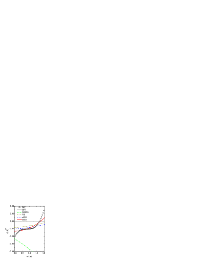
Figure 1: (Color online). Plot of the difference of contact values $g_{w}-g_{w}^{\text{SPT}}$ as a function of $\sigma$ for a polydisperse mixture with a top-hat distribution (30) with $c=0.2$ at a packing fraction $\eta=0.2$. The symbols are MC simulations.Ignacio The lines are SPT ($\cdots$), BGHLL (– $\cdot$ – $\cdot$), VS (– $\cdot\cdot$ – $\cdot\cdot$), eCS2 (– – –), and eCS3 (—).

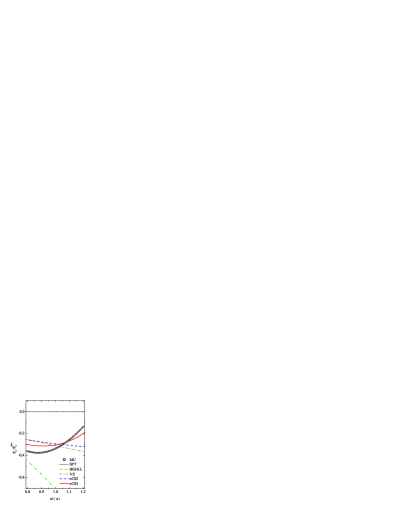
Figure 2: (Color online). Plot of the difference of contact values $g_{w}-g_{w}^{\text{SPT}}$ as a function of $\sigma$ for a polydisperse mixture with a top-hat distribution (30) with $c=0.2$ at a packing fraction $\eta=0.4$. The symbols are MC simulations.Ignacio The lines are SPT ($\cdots$), BGHLL (– $\cdot$ – $\cdot$), VS (– $\cdot\cdot$ – $\cdot\cdot$), eCS2 (– – –), and eCS3 (—).

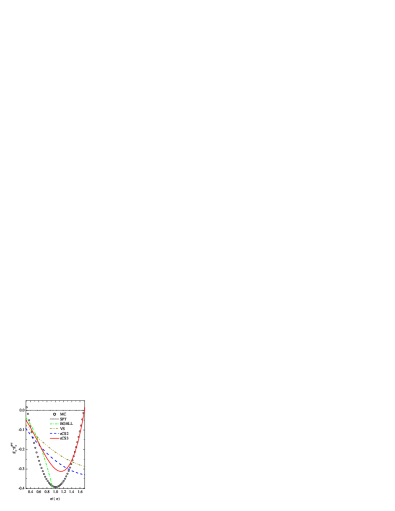
Figure 3: (Color online). Plot of the difference of contact values $g_{w}-g_{w}^{\text{SPT}}$ as a function of $\sigma$ for a polydisperse mixture with a top-hat distribution (30) with $c=0.7$ at a packing fraction $\eta=0.4$. The symbols are MC simulations.Ignacio The lines are SPT ($\cdots$), BGHLL (– $\cdot$ – $\cdot$), VS (– $\cdot\cdot$ – $\cdot\cdot$), eCS2 (– – –), and eCS3 (—).

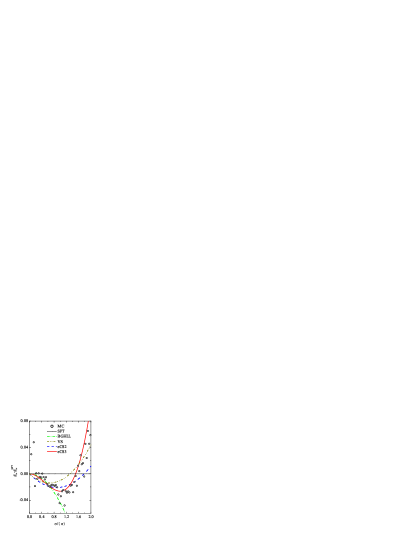
Figure 4: (Color online). Plot of the difference of contact values $g_{w}-g_{w}^{\text{SPT}}$ as a function of $\sigma$ for a polydisperse mixture with a Schulz distribution (31) with $q=5$ at a packing fraction $\eta=0.2$. The symbols are MC simulations.Ignacio The lines are SPT ($\cdots$), BGHLL (– $\cdot$ – $\cdot$), VS (– $\cdot\cdot$ – $\cdot\cdot$), eCS2 (– – –), and eCS3 (—).

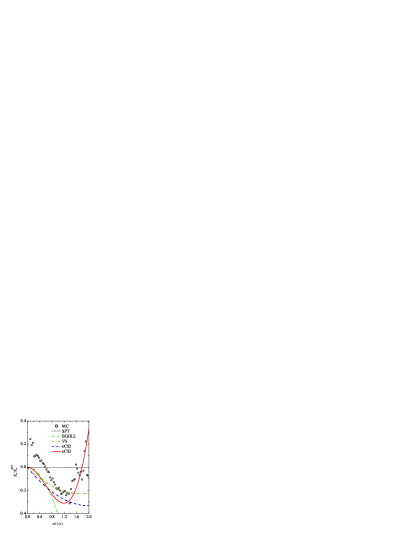
Figure 5: (Color online). Plot of the difference of contact values $g_{w}-g_{w}^{\text{SPT}}$ as a function of $\sigma$ for a polydisperse mixture with a Schulz distribution (31) with $q=5$ at a packing fraction $\eta=0.4$. The symbols are MC simulations.Ignacio The lines are SPT ($\cdots$), BGHLL (– $\cdot$ – $\cdot$), VS (– $\cdot\cdot$ – $\cdot\cdot$), eCS2 (– – –), and eCS3 (—).

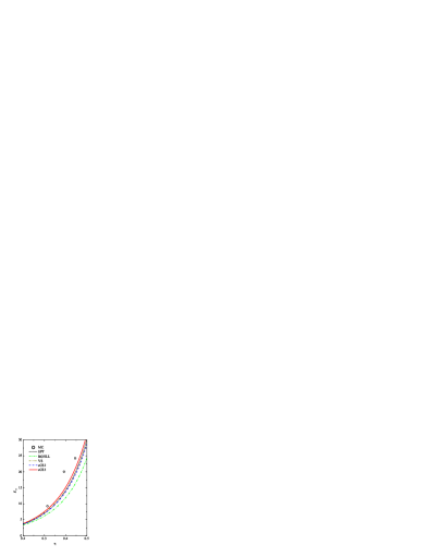
Figure 6: (Color online). Plot of the contact value $g_{11}(\sigma_{1})$ as a function of the packing fraction $\eta$ for the binary hard-sphere mixture $x_{1}=0.005$, $\sigma_{2}/\sigma_{1}=0.2$. The symbols are MC simulations.Cao et al. (2000) The lines are SPT ($\cdots$), BGHLL (– $\cdot$ – $\cdot$), VS (– $\cdot\cdot$ – $\cdot\cdot$), eCS2 (– – –), and eCS3 (—).

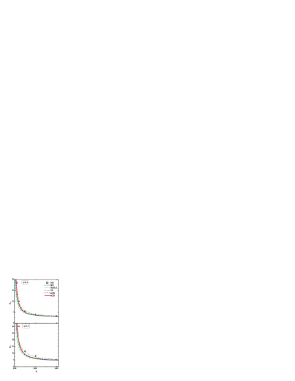
Figure 7: (Color online). Plot of the contact value $g_{11}(\sigma_{11})$ as a function of composition of the large spheres $x_{1}$ for two binary hard-sphere mixtures with $\sigma_{2}/\sigma_{1}=0.1$ and packing fractions $\eta=0.3$ (top panel) and $\eta=0.4$ (bottom panel), respectively. The symbols are molecular dynamics (MD) simulations.LW99 ; HTWC05 The lines are SPT ($\cdots$), BGHLL (– $\cdot$ – $\cdot$), VS (– $\cdot\cdot$ – $\cdot\cdot$), eCS2 (– – –), and eCS3 (—).

From Table 1 we observe that, among the approximations with $G_{3}=0$, only the SPT approximation yields a consistent EOS through the virial and the hard-wall routes, for any density and any degree of polydispersity. On the other hand, this internal consistency is at the expense of the rather poor quality of the SPT contact value $g_{\text{p}}^{\text{SPT}}$ in the one-component case. The PY, BGHLL, e1 and VS approximations are not consistent with $Z=Z_{w}$, even in the one-component limit (in which case $\mu_{n}\to\mu_{1}^{n}$). In the case of the e2 approximation, the inconsistency decreases with the degree of dispersity and disappears in the one-component limit.

It must be noted that the e1 approximation embodies the PY approximation as a particular case, i.e., the choice $g_{\text{p}}=g_{\text{p}}^{\text{PY}}$ yields $G^{\text{ePY1}}=G^{\text{PY}}$. Analogously, the SPT approximation can be recovered from e2 and e3: $g_{\text{p}}=g_{\text{p}}^{\text{SPT}}\Rightarrow G^{\text{eSPT2}}=G^{\text{eSPT3}}=G^{\text{SPT}}$.

Another comment is in order at this stage. From Eq. (12) we can observe that, for the class of approximations (11), the compressibility factor $Z$ does not depend on the individual values of the coefficients $G_{2}$ and $G_{3}$, but only on their sum. As a consequence, two different approximations of the form (11) sharing the same density dependence of $G_{1}$ and $G_{2}+G_{3}$ also share the same virial EOS. For instance, if one makes the choice $g_{\text{p}}=g_{\text{p}}^{\text{PY}}$, then $G^{\text{ePY3}}_{2}+G^{\text{ePY3}}_{3}=0$, see Eq. (22), and so $Z^{\text{ePY3}}=Z^{\text{PY}}$, even though $G^{\text{ePY3}}(z)\neq G^{\text{PY}}(z)$. Furthermore, if one makes the more sensible choice $g_{\text{p}}=g_{\text{p}}^{\text{CS}}$, then $G_{2}^{\text{eCS3}}+G_{3}^{\text{eCS3}}=G_{2}^{\text{BGHLL}}$, so that $Z^{\text{eCS3}}=Z^{\text{BMCSL}}$, but again $G^{\text{eCS3}}(z)\neq G^{\text{BGHLL}}(z)$.

III Comparison with Monte Carlo simulations

Buzzacchi et al.Ignacio have recently computed by Monte Carlo (MC) simulations the wall-particle contact value $g_{w}(\sigma)$ and the compressibility factor $Z$ for polydisperse hard spheres of packing fractions $\eta=0.2$ and $\eta=0.4$ with either a top-hat distribution of sizes given by

$$f(\sigma)=\begin{cases}1/2c,&\mu_{1}(1-c)\leq\sigma\leq\mu_{1}(1+c)\\ 0,&\text{otherwise}\end{cases}$$ (30)

or with a Schulz distribution of the form

$$f(\sigma)=\frac{q+1}{q!\mu_{1}}\left(\frac{q+1}{\mu_{1}}\sigma\right)^{q}\exp\left(-\frac{q+1}{\mu_{1}}\sigma\right).$$ (31)

In Table 2 we present the values of the parameters corresponding to the examined mixtures.

Table 3 compares the MC data of $Z$ for mixtures 1–5 with values obtained from different theoretical proposals by using both the virial and the wall routes. Here and it what follows, we have made the choice $g_{\text{p}}=g_{\text{p}}^{\text{CS}}$ in the approximations e1, e2, and e3. As indicated above, $Z^{\text{eCS3}}=Z_{w}^{\text{eCS3}}=Z^{\text{BMCSL}}$ and $Z^{\text{SPT}}=Z_{w}^{\text{SPT}}$. Note that $Z^{\text{BGHLL}}=Z^{\text{BMCSL}}$, but $Z_{w}^{\text{BGHLL}}\neq Z^{\text{BMCSL}}$. It can be observed from Table 3 that (apart from the SPT and the eCS3) the eCS2 and VS expressions for the contact values provide the least internal inconsistency between $Z$ and $Z_{w}$. We can also observe that $Z^{\text{BMCSL}}$, $Z^{\text{eCS1}}$, $Z^{\text{eCS2}}\simeq Z_{w}^{\text{eCS2}}$, and $Z^{\text{VS}}\simeq Z_{w}^{\text{VS}}$ are the most accurate EOS for the top-hat mixtures 1–3. On the other hand, the most accurate EOS for the Schulz cases 4 and 5 is $Z^{\text{SPT}}$.

Now we turn to the main topic of this paper, namely the contact values of the rdf. For the same polydisperse systems considered in Table 2, in Figs. 1–5 we show the comparison between the simulation resultsIgnacio for the wall-particle correlation function $g_{w}(\sigma)$ and those of different theories. Since all theories yield contact values which are increasing functions of $\sigma$, in order to emphasize features that would otherwise be difficult to ascertain, we have decided to represent the difference $g_{w}-g_{w}^{\text{SPT}}$ rather than $g_{w}$. The choice of $g_{w}^{\text{SPT}}$ as reference was motivated by the fact that it is the only previous theory consistent with the two ways of computing the pressure of the system. It is clear that the best overall performance in the comparison with the simulation data is given by $g_{w}^{\text{eCS3}}$, not only qualitatively but also quantitatively. Interestingly enough, $g_{w}^{\text{eCS2}}$ and $g_{w}^{\text{VS}}$ also do a good job in the cases of mixtures 1 (Fig. 1) and 4 (Fig. 4). In general, one can see that the SPT overestimates the contact values, except for high values of $\sigma$, and that the BGHLL prescription underestimates them. Also, although not included in the figure to avoid overcrowding, there is a very poor agreement of both $g_{w}^{\text{eCS1}}$ and $g_{w}^{\text{PY}}$ (which are linear in $z$) with the simulation data, both being underestimations.

While the main interest of our present formulation was geared towards the polydisperse system near a hard wall, Eq. (25), it should be clear that our new proposal for the contact values of the rdf also applies to the bulk fluid, Eq. (24). In particular, if the diameter distribution is discrete, the replacements $\sigma\to\sigma_{i}$ and $\sigma^{\prime}\to\sigma_{j}$ in Eq. (24) yield the contact values $g_{ij}(\sigma_{ij})$, where $i$ and $j$ denote the $i$-th and $j$-th species, respectively, and $\sigma_{ij}\equiv\left(\sigma_{i}+\sigma_{j}\right)/2$, with $\sigma_{k}$ denoting the diameter of a sphere of species $k$. Just to illustrate the kind of results our proposal produces, we consider two examples of binary hard-sphere mixtures. In the first case, we show in Fig. 6 a plot of the different theoretical predictions of $g_{11}(\sigma_{1})$ as a function of the packing fraction $\eta$, for a mixture having a mole fraction of the large spheres $x_{1}=0.005$, and a size ratio $\sigma_{2}/\sigma_{1}=0.2$, together with the simulation results of Cao et al.Cao et al. (2000) On the other hand, in Fig. 7 and for a binary mixture with $\sigma_{2}/\sigma_{1}=0.1$ and two values of the packing fraction ($\eta=0.3$ and $\eta=0.4$), we display the behavior of $g_{11}(\sigma_{1})$ as a function of the mole fraction of species $1$ derived from the various theories and the results of simulation by Lue and WoodcockLW99 and Henderson et al.HTWC05 It is again clear from Fig. 6 that $g_{11}^{\text{eCS3}}(\sigma_{1})$ gives the best performance for this mixture. As far as the behavior with respect to the mole fraction of the large spheres is concerned, as already noted by Henderson et al.,HTWC05 the approximation of Viduna and SmithVS02a does a very good job, especially for $\eta=0.4$, but it goes wrong for small values of $x_{1}$. Figure 7 also indicates that our proposal is certainly the best for $\eta=0.3$ and that it also accounts correctly for the sharp rise observed at the smallest values of the mole fraction of species $1$ for both packing fractions.

IV Concluding remarks

In this paper we have provided a new proposal for the contact values of the particle-particle correlation function, $g(\sigma,\sigma^{\prime})$, and of the wall-particle correlation function, $g_{w}(\sigma)$, of a hard-sphere fluid mixture with an arbitrary size distribution. The proposal relies on a kind of universality assumption by which, once the packing fraction is fixed, for all pairs of like and unlike spheres the dependence of the contact values on the diameters and on the composition is only through a single dimensionless parameter and holds for an arbitrary number of components. It also makes use of the point particle and the equal size limits and of the internal consistency between the usual virial route and the hard-wall limit route to derive the pressure of the system. As a consequence, the contact value $g_{\text{p}}$ of the rdf of a one-component fluid is required as the only input, thus making the formulation to be both simple and rather flexible.

The merits of this proposal have been assessed by comparing the contact values themselves and the corresponding compressibility factors with other theoretical developments and with recent MC simulation results both for polydisperse hard-sphere fluids at a hard wall and for binary hard-sphere mixtures (discrete size distribution). It is fair to say that the new proposal with the CS expression for $g_{\text{p}}$ gives the best overall performance. Also it is clear that (i) two different approximations $g(\sigma,\sigma^{\prime})$ for the contact values can yield the same compressibility factor $Z$ and (ii) a fortunate cancelation of errors can make a poor approximation for $g(\sigma,\sigma^{\prime})$ to lead to a reliable $Z$. Examples of the first effect are provided by the approximations PY and ePY3, which differ at the level of the contact values but share the same EOS, and, similarly, by the approximations BGHLL and eCS3. An example of the second effect is represented by the eCS1 approximation, which yields a very accurate EOS,Santos et al. (1999) even though the associated contact values are only qualitatively correct.

In previous work of ours we have attempted to provide expressions for the contact values of the rdf and the compressibility factors that are valid for any dimensionality $d$.Santos et al. (1999, 2002) The present proposal does not fulfill such a condition. It will also work for $d=1$ and $d=2$, but it is not directly generalizable to arbitrary $d$.LS04

Apart from the EOS, contact values of the rdf may also be useful in other contexts. For instance, they are required as input in the rational function approximation approach to the structural properties of hard-sphere mixtures.YSH98 We plan to use them in connection with this problem in the near future.

- (1) For a proof on the equivalence between the energy and virial routes to the equation of state of hard-sphere fluids, see A. Santos, J. Chem. Phys. 123, 104102 (2005).
- Lebowitz (1964) J. L. Lebowitz, Phys. Rev. A 133, 895 (1964).
- Boublík (1970) T. Boublík, J. Chem. Phys. 53, 471 (1970).
- Mansoori et al. (1971) G. A. Mansoori, N. F. Carnahan, K. E. Starling, and J. T. W. Leland, J. Chem. Phys. 54, 1523 (1971).
- Grundke and Henderson (1972) E. W. Grundke and D. Henderson, Mol. Phys. 24, 269 (1972).
- Lee and Levesque (1973) L. L. Lee and D. Levesque, Mol. Phys. 26, 1351 (1973).
- Lebowitz et al. (1965) J. L. Lebowitz, E. Helfand, and E. Praestgaard, J. Chem. Phys. 43, 774 (1965).
- Rosenfeld (1988) Y. Rosenfeld, J. Chem. Phys. 89, 4272 (1988).
- (9) D. Henderson, A. Malijevský, S. Labík, and K.-Y. Chan, Mol. Phys. 87, 273 (1996); D. H. L. Yau, K.-Y. Chan, and D. Henderson, ibid. 88, 1237 (1996); 91, 1813 (1997); D. Henderson and K.-Y. Chan, J. Chem. Phys. 108, 9946 (1998); Mol. Phys. 94, 253 (1998); D. Matyushov, D. Henderson, and K.-Y. Chan, ibid. 96, 1813 (1999); D. Henderson and K.-Y. Chan, ibid. 98, 1005 (2000).
- (10) D. V. Matyushov and B. M. Ladanyi, J. Chem. Phys. 107, 5815 (1997)
- Barrio and Solana (2000) C. Barrio and J. R. Solana, J. Chem. Phys. 113, 10180 (2000).
- Santos et al. (1999) A. Santos, S. B. Yuste, and M. López de Haro, Mol. Phys. 96, 1 (1999).
- Santos et al. (2002) A. Santos, S. B. Yuste, and M. López de Haro, J. Chem. Phys. 117, 5785 (2002).
- (14) A. Vrij, J. Chem. Phys. 69, 1742 (1978); L. Blum and G. Stell, ibid. 71, 3714 (1979); J. A. Gualtieri, J. M. Kincaid, and G. Morrison, ibid. 77, 521 (1982); J. J. Salacuse and G. Stell, ibid. 77, 3714 (1982); W. L. Griffith, R. Triolo, and A. L. Compere, Phys. Rev. A 33, 2197 (1986); D. A. Kofke and E. Glandt, J. Chem. Phys. 87, 4881 (1987); 90, 439 (1989); J. M. Kincaid, R. A. McDonald, and G. Morrison, ibid. 87, 5425 (1987); J. M. Kincaid, M. López de Haro, and E. G. D. Cohen, Int. J. Thermophys. 9, 1031 (1988).
- (15) See, for instance, P. Sollich and M. E. Cates, Phys. Rev. Lett. 80, 1365 (1998); C. Tutschka and G. Kahl, J. Chem. Phys. 108, 9498 (1998); J. Zhang, R. Blaak, E. Trizac, J. A. Cuesta, and D. Frenkel, ibid. 110, 5318 (1999); P. Bryk, A. Patrykiejew, J. Reszko-Zygmunt, and S. Sokolowski, ibid. 111, 6047 (1999); P. Bartlett, Mol. Phys. 97, 685 (1999); J. A. Cuesta, Europhys. Lett. 47, 197 (1999); D. A. Kofke and P. G. Bolhuis, Phys. Rev. E 59, 618 (1999); M. Ginoza and M. Yasutomi, ibid. 59, 2060 (1999); 59, 3270 (1999); R. P. Sear, Phys. Rev. Lett. 82, 4244 (1999); I. Pagonabarraga, M. E. Cates, and G. J. Ackland, ibid. 84, 911 (2000); R. Blaak, J. Chem. Phys. 112, 9041 (2000); R. P. Sear, ibid. 113, 4732 (2000); D. Gazzillo and A. Giacometti, ibid. 113, 9837 (2000); R. Blaak and J. A. Cuesta, ibid. 115, 963 (2001); P. Sollich, P. B. Warren, and M. E. Cates, Adv. Chem. Phys. 116, 265 (2001); P. Sollich, J. Phys.: Condens. Matter 14, R79 (2002); N. B. Wilding and P. Sollich, J. Chem. Phys., 116, 7116 (2002); M. Fasolo and P. Sollich, Phys. Rev. Lett. 91, 068301 (2003); C. C. Huang and H. Xu, Mol. Phys. 102, 967 (2004); Y.-X. Yu, J. Wu, Y.-X. Xin, and G.-H. Gao, J. Chem. Phys. 121, 1535 (2004); S. Leroch, D. Gottwald, and G. Kahl, Condensed Matter Physics 7, 301 (2004).
- (16) M. Buzzacchi, I. Pagonabarraga, and N. B. Wilding, J. Chem. Phys. 121, 11362 (2004).
- (17) F. Lado, Phys. Rev. E 54, 4411 (1996).
- (18) R. Evans, in Liquids and Interfaces, edited by J. Charvolin, J. F. Joanny, and J. Zinn-Justin (North-Holland, Amsterdam, 1990).
- Carnahan and Starling (1969) N. F. Carnahan and K. E. Starling, J. Chem. Phys. 51, 635 (1969).
- (20) D. Viduna and W. R. Smith, Mol. Phys. 100, 2903 (2002).
- Cao et al. (2000) D. Cao, K.-Y. Chan, D. Henderson, and W. Wang, Mol. Phys. 98, 619 (2000).
- (22) L. Lue and L. V. Woodcock, Mol. Phys. 96, 1435 (1999).
- (23) D. Henderson, A. Trokhymchuk, L. V. Woodcock, and K.-Y. Chan, Mol. Phys. 103, 667 (2005).
- (24) For , the approximations e1, e2, and e3 reduce to the exact result . For , the approximations e3 and e2 become identical because the latter already fulfills the condition , as shown by S. Luding and A. Santos, J. Chem. Phys. 121, 8458 (2004). It is tempting to speculate that a polynomial form for of degree could be found to be consistent with the condition for . However, a more detailed analysis shows that this is not the case since the number of conditions exceeds the number of unknowns, unless the universality assumption is partially relaxed.
- (25) S. B. Yuste, A. Santos, and M. López de Haro, J. Chem. Phys. 108, 3683 (1998).