The Smeagol method for spin- and molecular-electronics

Abstract

Ab initio computational methods for electronic transport in nanoscaled systems are an invaluable tool for the design of quantum devices. We have developed a flexible and efficient algorithm for evaluating $I$-$V$ characteristics of atomic junctions, which integrates the non-equilibrium Green’s function method with density functional theory. This is currently implemented in the package Smeagol. The heart of Smeagol is our novel scheme for constructing the surface Green’s functions describing the current/voltage probes. It consists of a direct summation of both open and closed scattering channels together with a regularization procedure of the Hamiltonian, and provides great improvements over standard recursive methods. In particular it allows us to tackle material systems with complicated electronic structures, such as magnetic transition metals. Here we present a detailed description of Smeagol together with an extensive range of applications relevant for the two burgeoning fields of spin and molecular-electronics.

I Introduction

The study of electronic transport through devices comprising only a handful of atoms is becoming one of the most fascinating branch of modern solid state physics. The field was initiated with the advent of the scanning tunnelling microscope (STM) STM and at present comprises a multitude of applications which span over several disciplines and encompass different technologies, from building blocks for revolutionary computer architectures, to disposable electronics, to diagnostic tools for genetically driven medicine. Clearly many of these devices will soon change and enhance the quality of our daily life.

Fully functional molecular memories memory and logic gates gates1 ; gates2 have been already demonstrated suggesting a possible roadmap to the post-silicon era. These should produce future generations of computers, together with magnetic data storage devices exceeding the Terabit/in² storage limit. The readout of such high-density data storage media will be achieved using nanoscale devices with magnetic atomic point contacts PC1 ; PC2 .

At the same time hybrid molecular devices are becoming increasingly popular in multifunctional sensor design, demonstrating a sensitivity orders of magnitude superior to that achievable with conventional methods. These molecular devices include for example carbon nanotubes detectors for NO₂ NO2 and nerve agents nerve , nanowire-based virus detectors virus and chemical sensors chem . The near future should see the development of on-chip nanolabs able to sense a particular signature of gene or protein expression and therefore be able to diagnose various diseases. These will be formidable tools for the study of biological systems and in the field of preventive medicine med .

In addition to this large experimental activity an equally large effort has been devoted to the development of efficient computational methods for evaluating $I$-$V$ characteristics of nanoscale devices. This is quite a remarkable theoretical challenge since advanced quantum transport algorithms must be combined with state of the art electronic structure methods. Ideally these tools should be able to include strong correlation as well as inelastic effects, and they should be suitable for describing large systems (easily scalable methods). Furthermore in order to compare directly to experiments the detailed knowledge of the atomic configuration is needed.

Modern theory of quantum transport has developed a range of methods for calculating transport in nanoscale conductors. Broadly speaking these can be divided into two main classes: 1) steady state algorithms, and 2) time dependent schemes. The first are based upon the assumption that, regardless of the details of a possible transient, a steady state is always achieved. The current through the entire device is calculated as a balance of currents entering and leaving a given scattering region, either using scattering theory GF1 ; GF2 ; GF3 ; GF4 ; WF1 ; WF2 ; WF3 , or by solving a master equation ME1 ; ME2 ; ME3 . A multitude of variations over this generic scheme are available StefRev , depending on the underlying assumption leading to the steady state, the details of the electronic structure method employed, and the way in which the external potential is introduced in the calculation. Interestingly most of the methods can be demonstrated to be applicable to cases of non-interacting electrons stef1 , although their equivalence is not demonstrated for the interacting case. Among these algorithms a particular place is occupied by implementations of the non-equilibrium Green function (NEGF) GF1 ; GF2 ; GF3 ; GF4 method within density functional theory (DFT) DFT ; KohnSham . This approach, which is based on equilibrium DFT to describe the electronic structures, has the advantage of being conceptually simple, and computationally easy and versatile to implement NEGF1 ; NEGF2 ; NEGF3 ; NEGF4 ; NEGF5 .

Time dependent methods are at an earlier stage of development. These investigate the time-evolution of the electronic charge density of a system, brought out of equilibrium by a time-dependent perturbing potential. To the best of our knowledge two fundamentally different methods have been proposed to date. The first considers infinite non-periodic systems, with an external potential introduced as a time dependent perturbation stef1 ; cini . The time-evolution of the density matrix is studied with time-dependent density functional theory (TDDFT) Gross ; TDDFT . An alternative approach consists of placing the system of interest in a large capacitor. Such a capacitor is charged at $t$=0 and the time-dependent de-charging process is investigated Tchav ; Max1 . Generally speaking these methods are computationally intensive, since the need to perform the time evolution adds to the computational overheads of standard static schemes. However they should be able to address transport limits such as Coulomb blockade or resonant tunnelling, which are otherwise difficult to describe. Interestingly, important information can be extracted from the static limit of the time-dependent problem Max2 ; Kieron1 , and this can help in designing more accurate static methods and in understanding their limitations.

Here we present in details our recently developed quantum transport code Smeagol Smeagol1 . Smeagol is a DFT implementation of the non-equilibrium Green’s function method, which has been specifically designed for magnetic materials. The main core of Smeagol is our original technique for constructing the leads self-energies rgf , which avoids the standard problems of recursive methods GF1 and allows us to describe devices having current/voltage probes with a complicated electronic structure. In addition Smeagol has been constructed to be a modular and scalable code, with particular emphasis on heavy parallelization, to facilitate large scale simulations. In its present form Smeagol is parallel over $k$-space, real space and energy and furthermore it can deal with spin-polarised systems, including spin non-collinearity. A partial description of the code has already been provided Smeagol2 , which should be incorporated with this more detailed description.

The paper is organized as follows. In the next section we introduce our method and its main technical implementations. In particular we set the problem, explain how to construct the leads self-energies, and describe the strategy used for calculating the electrostatic potential. Then we present a series of calculations for systems relevant to either spin- or molecular-electronics. These address specific aspects of Smeagol such as the electrostatics, the spin polarization and the spin non-collinearity. Finally in the appendices we describe in more details the self-energy algorithm, we recall the theoretical foundations of the NEGF formalism, and we establish a connection with TDDFT.

II Non-equilibrium transport method

In this section we describe in details our computational technique. The underlying assumption used throughout this work is that all the quantities associated to the electronic structure (Hamiltonian, density matrix, Green’s functions, etc.) can be written over a localized atomic orbital (LAO) basis set of some kind $\psi_{i\>\mu}=\psi_{\mu}(\vec{r}-\vec{R}_{i})$, where $\vec{R}_{i}$ is the position of the $i$-th nucleus and $\mu=n,l,m$ is a collective index spanning, the angular momentum ($l,m$) and the orbital $n$. Note that in general the index $n$ can run over different radial functions corresponding to the same angular momentum, according to the multiple-zetas scheme MZ . In this way a generic operator $\hat{O}$ is represented by a finite $N\times N$ matrix ($N$ is the total number of degrees of freedom in the system) whose matrix elements are simply $O_{i\>\mu,\leavevmode\nobreak\ j\nu}$. Note also that the functions $\psi_{i\>\mu}$ are generally non-orthogonal and the overlap matrix $S$ is defined as $S_{i\>\mu,\leavevmode\nobreak\ j\nu}=\int\psi_{\mu}^{*}(\vec{r}-\vec{R}_{i})\psi_{\nu}(\vec{r}-\vec{R}_{j})\>\mathrm{d}^{3}\vec{r}$.

II.1 Problem setup

Smeagol has been designed to describe two-terminal conductance experiments, where two current/voltage electrodes of macroscopic size sandwich a nanometer-sized device (a molecule, an atomic point contact, a tunneling barrier…). Let us present the problem from three different perspectives: the thermodynamics, the Hamiltonian and the electrostatics (see figure 1).

Figure 1: Schematic two terminal device. (a) Thermodynamical aspect: two leads are kept respectively at the chemical potentials $\mu_{\mathrm{L}}$ and $\mu_{\mathrm{R}}$ and are able to exchange electrons with the central region (extended molecule EM). (b) Hamiltonian description: two block diagonal infinite matrices describe the semi-infinite current/voltage probes, and a finite matrix $H_{\mathrm{M}}$ describes the extended molecule. $H_{0}$ is a finite Hamiltonian matrix describing one principal layer, while $H_{1}$ describes the interaction between two adjacent principal layers. (c) Electrostatics: the two current/voltage leads have a constant average potential $\mu_{\mathrm{L/R}}=E_{\mathrm{F}}\pm V/2$, and the potential drop occurs within the extended molecule.

From a thermodynamic point of view the system is modelled two bulk leads and a central region. The latter includes the actual device and, for reasons that will be clear later, part of the leads. Therefore we call such a central region an “extended molecule” (EM). The two current/voltage leads are kept at two different chemical potentials respectively $\mu_{\mathrm{L}}$ and $\mu_{\mathrm{R}}$ and are able to exchange electrons with the EM. Note that when the applied bias is zero ($\mu_{\mathrm{L}}=\mu_{\mathrm{R}}$), this system of interacting electrons is in thermodynamic equilibrium and may be regarded as a grand canonical ensemble. When the bias is applied however $\mu_{\mathrm{L}}\neq\mu_{\mathrm{R}}$ and the current will flow. Then the prescription for establishing the steady state is that of adiabatically switching on the coupling between the leads and the EM GF3 ; KEL1 ; KEL2 .

At the Hamiltonian level the system under investigation is described by an infinite hermitian matrix ${\cal H}$. This however has a rather regular structure. First notice that the two semi-infinite current/voltage probes are defect-free crystalline metals. These have a regular periodic structure and a unit cell along which the direction of the transport can be defined. At this point it is important to notice that because of the LAO basis set this matrix will be rather sparse. It is convenient to introduce the concept of principal layer (PL). A principal layer is the smallest cell that repeats periodically in the direction of the transport constructed in such a way to interact only with the nearest neighbour PLs. This means that all the matrix elements between atoms belonging to two non-adjacent PLs vanish. For example take a linear chain of hydrogen atoms described by a nearest neighbour tight-binding model then one atom forms the unit cell. However if nearest and next nearest neighbour elements are included then the PL will contain two atoms etc (for examples see appendix A).

We then define $H_{0}$ as the $N\times N$ matrix describing all interactions within a PL, where $N$ is the total number of degrees of freedom (basis functions) in the PL (note that we use calligraphic symbols - ${\cal H}$ - for infinitely-dimensional matrices and capitalized letters - $H$ - for finite matrices). Similarly $H_{1}$ is the $N\times N$ matrix describing the interaction between two PLs. Finally $H_{\mathrm{M}}$ is the $M\times M$ matrix describing the extended molecule and $H_{\mathrm{LM}}$ ($H_{\mathrm{RM}}$) is the $N\times M$ matrix containing the interaction between the last PL of the left-hand side (right-hand side) lead and the extended molecule. The final form of ${\cal H}$ is

$${\cal H}=\left(\begin{array}[]{ccccccccccc}.&.&.&.&.&.&.&.&.&.&\\ .&0&H_{-1}&H_{0}&{H}_{1}&0&.&.&.&.&.\\ .&.&0&H_{-1}&H_{0}&{H}_{\mathrm{LM}}&0&.&.&.&.\\ .&.&.&0&H_{\mathrm{ML}}&H_{\mathrm{M}}&H_{\mathrm{MR}}&0&.&.&.\\ .&.&.&.&0&H_{\mathrm{RM}}&H_{0}&H_{1}&0&.&.\\ .&.&.&.&.&0&H_{-1}&H_{0}&H_{1}&0&.\\ .&.&.&.&.&.&.&.&.&.&.\\ \end{array}\right)\;.$$ (1)

For a system which preserves time-reversal symmetry $H_{-1}=H_{1}^{\dagger}$, $H_{\mathrm{ML}}=H_{\mathrm{LM}}^{\dagger}$ and $H_{\mathrm{MR}}=H_{\mathrm{RM}}^{\dagger}$. In this form ${\cal H}$ has the same structure as the Hamiltonian of a one-dimensional system as shown in figure 1b. However this is not the most general situation and does not apply if a magnetic field is present for example.

Note that the overlap matrix ${\cal S}$ has exactly the same structure of ${\cal H}$. Therefore we adopt the notation $S_{0}$, $S_{1}$, $S_{\mathrm{LM}}$, $S_{\mathrm{RM}}$ and $S_{\mathrm{M}}$ for the various blocks of ${\cal S}$, in complete analogy with their Hamiltonian counterparts. Here the principal layer, defined by ${\cal H}$ is used for both the ${\cal S}$ and the ${\cal H}$ matrix, even though the range of ${\cal S}$ can be considerably shorter than that of ${\cal H}$.

Let us now discuss the electrostatics of the problem (figure 1c). The main consideration here is that the current/voltage probes are made from good metals and therefore preserve local charge neutrality. For this reason the effect of an external bias voltage on the leads will produce a rigid shift of the whole spectrum, i.e. of all the on-site energies. In contrast a non-trivial potential profile will develop over the extended molecule, which needs to be calculated self-consistently. Importantly the resulting self-consistent electrostatic potential must match that of the leads at the boundaries of the EM. If this does not happen, the potential profile will develop a discontinuity with the generation of spurious scattering. Therefore, in order to achieve a good match of the electrostatic potential, several layers of the leads are usually included in the extended molecule. Their number ultimately depends upon the screening length of the leads, but in most situations a few (between two and four) atomic planes are sufficient.

Even in the case of extremely short screening length, it is however good practice to include a few planes of the leads in the extended molecule because the electrodes generally have reconstructed surfaces, which might undergo additional geometrical reconstructions when bonding to the nanoscale device (e.g. molecules attached to metallic surfaces through corrosive chemical groups).

We conclude this section with some comments about the application of periodic boundary conditions in the transverse direction perpendicular to that of the transport. The setup of a typical experiment is that of two very large current voltage probes sandwiching a tiny region which is responsible for most of the resistance. The ideal description would be that of two infinite leads (with infinite cross sections) and a finite scattering region. Unfortunately this problem is intractable since both $H_{0}$ and $H_{1}$ become infinitely-dimensional. Therefore one has to consider some approximations.

The first option is to use leads with finite cross section. In this case, no periodic boundary conditions are required and the whole system is quasi-one-dimensional. However special care must be taken when choosing the cross section of the leads in order to avoid quantum confinement effects. It is also worth noting that leads with very small cross section make the use of the Landauer formula for transport LBYP questionable. As a rule of thumb the linear dimension of the cross section should be several times the Fermi wavelength of the material forming the leads and there should be several open scattering channels.

The second option is to use periodic boundary conditions. In this case the system is repeated periodically in the transverse direction, meaning that the extended molecule is also repeated periodically. Clearly quantum confinement effects are eliminated, but one should be particularly careful in order to eliminate the spurious interaction between the mirror images of the extended molecule. Therefore large unit cells must be employed even when periodic boundary conditions are used. However from a formal point of view the use of periodic boundary conditions does not change the problem setup. All the matrices ($H_{0}$, $H_{1}$ etc.) now depend on the transverse $k$-vector used, and the infinite problem transforms in a collection of $k$-dependent quasi one-dimensional problems. This dependence is implicitly assumed whenever necessary throughout the rest of the paper.

II.2 Green’s functions for an open system

We are dealing with an infinite-dimensional hermitian problem, which is intractable, because the wave-functions deep inside the leads have a plane-wave form. These can be calculated by computing the band-structure of an infinite chain of PL’s. The main computational effort is therefore focussed upon the problem of describing the scattering of plane-waves from one lead to the other across the EM. The problem is solved by computing the retarded Green’s function ${\cal G}^{\mathrm{R}}$ for the whole system by solving the Green’s function equation

$$[\epsilon^{+}{\cal S}-{\cal H}]\>{\cal G}^{\mathrm{R}}(E)={\cal I}\>,$$ (2)

where ${\cal I}$ is an infinitely-dimensional identity matrix, $\epsilon^{+}=\lim_{\delta\rightarrow 0^{+}}E+i\delta$ and $E$ is the energy. The same equation explicitly using the block-diagonal structure of both the Hamiltonian and the overlap matrix (we drop the symbol “R” indicating the retarded quantities) is of the form

$$\left(\begin{array}[]{ccc}\epsilon^{+}{\cal S}_{\mathrm{L}}-{\cal H}_{\mathrm{L}}&\epsilon^{+}{\cal S}_{\mathrm{LM}}-{\cal H}_{\mathrm{LM}}&0\\ \epsilon^{+}{\cal S}_{\mathrm{ML}}-{\cal H}_{\mathrm{ML}}&\epsilon^{+}S_{\mathrm{M}}-H_{\mathrm{M}}&\epsilon^{+}{\cal S}_{\mathrm{MR}}-{\cal H}_{\mathrm{MR}}\\ 0&\epsilon^{+}{\cal S}_{\mathrm{RM}}-{\cal H}_{\mathrm{RM}}&\epsilon^{+}{\cal S}_{\mathrm{R}}-{\cal H}_{\mathrm{R}}\\ \end{array}\right)\left(\begin{array}[]{ccc}{\cal G}_{\mathrm{L}}&{\cal G}_{\mathrm{LM}}&{\cal G}_{\mathrm{LR}}\\ {\cal G}_{\mathrm{ML}}&G_{\mathrm{M}}&{\cal G}_{\mathrm{MR}}\\ {\cal G}_{\mathrm{RL}}&{\cal G}_{\mathrm{RM}}&{\cal G}_{\mathrm{R}}\\ \end{array}\right)=\left(\begin{array}[]{ccc}{\cal I}&0&0\\ 0&I_{\mathrm{M}}&0\\ 0&0&{\cal I}\\ \end{array}\right)\;,$$ (3)

where we have partitioned the Green’s functions ${\cal G}$ into the infinite blocks describing the left- and right-hand side leads ${\cal G}_{\mathrm{L}}$ and ${\cal G}_{\mathrm{R}}$, those describing the interaction between the leads and extended molecule ${\cal G}_{\mathrm{LM}}$, ${\cal G}_{\mathrm{RM}}$, the direct scattering between the leads ${\cal G}_{\mathrm{LR}}$, and the finite block describing the extended molecule $G_{\mathrm{M}}$. We have also introduced the matrices ${\cal H}_{\mathrm{L}}$, ${\cal H}_{\mathrm{R}}$, ${\cal H}_{\mathrm{LM}}$, ${\cal H}_{\mathrm{RM}}$ and their corresponding overlap matrix blocks, indicating respectively the left- and right-hand side leads Hamiltonian and the coupling matrix between the leads and the extended molecule. $H_{\mathrm{M}}$ is an $M\times M$ matrix and $I_{\mathrm{M}}$ is the $M\times M$ unit matrix. The infinite matrices, ${\cal H}_{\mathrm{L}}$ and ${\cal H}_{\mathrm{R}}$ describe the leads and have the following block-diagonal form

$${\cal H}_{\mathrm{L}}=\left(\begin{array}[]{ccccc}\ddots&\ddots&\ddots&\ddots&\vdots\\ 0&H_{-1}&H_{0}&H_{1}&0\\ \dots&0&H_{-1}&H_{0}&H_{1}\\ \dots&\dots&0&H_{-1}&H_{0}\\ \end{array}\right)\>,$$ (4)

with similar expressions for ${\cal H}_{\mathrm{R}}$ and the overlap ${\cal S}$ matrix counterparts. In contrast the coupling matrices between the leads and the extended molecule are infinite dimensional matrices whose elements are all zero except for a rectangular block coupling the last PL of the leads and the extended molecule. For example we have

$${\cal H}_{\mathrm{LM}}=\left(\begin{array}[]{c}\vdots\\ 0\\ H_{\mathrm{LM}}\\ \end{array}\right)\>.$$ (5)

The crucial step in solving equation (3) is to write down the corresponding equation for the Green’s function involving the EM and surface PL’s of the left and right leads and then evaluate the retarded Green’s function for the extended molecule $G_{\mathrm{M}}^{\mathrm{R}}$. This has the form

$$G_{\mathrm{M}}^{\mathrm{R}}(E)=\left[\epsilon^{+}S_{\mathrm{M}}-H_{\mathrm{M}}-\Sigma_{\mathrm{L}}^{\mathrm{R}}(E)-\Sigma_{\mathrm{R}}^{\mathrm{R}}(E)\right]^{-1}\>,$$ (6)

where we have introduced the retarded self-energies for the left- and right-hand side lead

$$\Sigma_{\mathrm{L}}^{\mathrm{R}}(E)=(\epsilon^{+}S_{\mathrm{ML}}-H_{\mathrm{ML}})G_{\mathrm{L}}^{0\mathrm{R}}(E)\>(\epsilon^{+}S_{\mathrm{LM}}-H_{\mathrm{LM}})\>$$ (7)

and

$$\Sigma_{\mathrm{R}}^{\mathrm{R}}(E)=(\epsilon^{+}S_{\mathrm{MR}}-H_{\mathrm{MR}})G_{\mathrm{R}}^{0\mathrm{R}}(E)\>(\epsilon^{+}S_{\mathrm{RM}}-H_{\mathrm{RM}})\>.$$ (8)

Here $G_{\mathrm{L}}^{0\mathrm{R}}$ and $G_{\mathrm{R}}^{0\mathrm{R}}$ are the retarded surface Green’s function of the leads, i.e. the leads retarded Green’s functions evaluated at the PL neighboring the extended molecule. Formally $G_{\mathrm{L}}^{0\mathrm{R}}$ ($G_{\mathrm{R}}^{0\mathrm{R}}$) corresponds to the right lower (left higher) block of the retarded Green’s function for the whole left-hand side (right-hand side) lead. These are simply

$${\cal G}_{\mathrm{L}}^{0\mathrm{R}}(E)=[\epsilon^{+}{\cal S}_{\mathrm{L}}-{\cal H}_{\mathrm{L}}]^{-1}\>$$ (9)

and

$${\cal G}_{\mathrm{R}}^{0\mathrm{R}}(E)=[\epsilon^{+}{\cal S}_{\mathrm{R}}-{\cal H}_{\mathrm{R}}]^{-1}\>.$$ (10)

Note that ${\cal G}_{\mathrm{L}}^{0\mathrm{R}}$ (${\cal G}_{\mathrm{R}}^{0\mathrm{R}}$) is not the same as ${\cal G}_{\mathrm{L}}^{\mathrm{R}}$ (${\cal G}_{\mathrm{R}}^{\mathrm{R}}$) defined in equation (3). In fact the former are the Green’s functions for the semi-infinite leads in isolation, while the latter are the same quantities for the leads attached to the scattering region. Importantly one does not need to solve the equations (9) and (10) for calculating the leads surface Green’s functions and a closed form avoiding the inversion of infinite matrices can be provided rgf . This will be discussed in what follows and in appendix A.

Let us conclude this section with a few comments on the results obtained. The retarded Green’s function $G_{\mathrm{M}}^{\mathrm{R}}$ contains all the information about the electronic structure of the extended molecule attached to the leads. In its close form given by the equation (6) it is simply the retarded Green’s function associated to the effective Hamiltonian matrix $H_{\mathrm{eff}}$

$$H_{\mathrm{eff}}=H_{\mathrm{M}}+\Sigma_{\mathrm{L}}^{\mathrm{R}}(E)+\Sigma_{\mathrm{R}}^{\mathrm{R}}(E)\>.$$ (11)

Note that $H_{\mathrm{eff}}$ is not hermitian since the self-energies are not hermitian matrices. This means the the number of particles in the extended molecule is not conserved, as expected by the presence of the leads. Moreover, since $G_{\mathrm{M}}^{\mathrm{R}}$ contains all the information about the electronic structure of the extended molecule in equilibrium with the leads, it can be directly used for extracting the zero-bias conductance $G$ of the system. In fact one can simply apply the Fisher-Lee GF1 ; fisherlee relation and obtain

$$G=\frac{2e^{2}}{h}\mathrm{Tr}[\Gamma_{\mathrm{L}}\>G^{\mathrm{R\dagger}}_{\mathrm{M}}\>\Gamma_{\mathrm{R}}\>G^{\mathrm{R}}_{\mathrm{M}}]\>,$$ (12)

where

$$\Gamma_{\alpha}(E)=i[\Sigma^{\mathrm{R}}_{\alpha}(E)-\Sigma^{\mathrm{R}}_{\alpha}(E)^{\dagger}]\>.$$ (13)

In equation (12) all the quantities are evaluated at the Fermi energy $E_{\mathrm{F}}$. Clearly $\mathrm{Tr}[\Gamma_{\mathrm{L}}\>G^{\mathrm{R\dagger}}_{\mathrm{M}}\>\Gamma_{\mathrm{R}}\>G^{\mathrm{R}}_{\mathrm{M}}](E)$ is simply the energy dependent total transmission coefficient $T(E)$ of standard scattering theory LBYP .

Finally note that what we have elaborated so far is an alternative way of solving a scattering problem. In standard scattering theory one first computes the asymptotic current carrying states deep into the leads (scattering channels) and then evaluate the quantum mechanical probabilities for these channels to be reflected and transmitted through the extended molecule LBYP . In this case the details of the scattering region are often reduced to a matrix describing the effective coupling between the two surface PLs of the leads rgf . In contrast the use of (12) describes an alternative though equivalent approach, in which the leads are projected out to yield a reduced matrix describing an effective EM. The current through surface PL’s perpendicular to the transport direction are the same TCH1 , the two approaches are equivalent and there is no clear advantage in using either one or the other. However, when the Hamiltonian matrix of the scattering region $H_{\mathrm{M}}$ is not known a priori, then the NEGF method offers a simple way of setting up a self-consistent procedure.

II.3 Steady-state and self-consistent procedure

Consider now the case in which the matrix elements of the Hamiltonian of the system are not known explicitly, but only their functional dependence upon the charge density $\rho$, ${\cal H}={\cal H}[\rho]$, is known. This is the most common case in standard mean field electronic structure theory, such as DFT. If no external bias is applied to the device (linear response limit) the Hamiltonian of the system can be simply obtained from a standard equilibrium DFT calculation and the procedure described in the previous section can be applied without any modification. However, when an external bias $V$ is applied, the charge distribution of the extended molecule will differ from that at equilibrium since both the net charge and the electrical polarization are affected by the bias. This will determine a new electrostatic potential profile with different scattering properties.

These modifications will affect only the extended molecule, since our leads are required to preserve local charge neutrality. This means that the charge density and therefore the Hamiltonian of the leads are not modified by the external bias applied. As discussed at the beginning the only effect of the external bias over the current/voltage electrodes is that of a rigid shift of the on-site energies. The Hamiltonian then takes the form

$${\cal H}=\left(\begin{array}[]{ccc}{\cal H}_{\mathrm{L}}+{\cal I}\>eV/2&{\cal H}_{\mathrm{LM}}&0\\ {\cal H}_{\mathrm{ML}}&H_{\mathrm{M}}&{\cal H}_{\mathrm{MR}}\\ 0&{\cal H}_{\mathrm{RM}}&{\cal H}_{\mathrm{R}}-{\cal I}\>eV/2\\ \end{array}\right)\>,$$ (14)

Note that the coupling matrices between the leads and the extended molecule are also not modified by the external bias, since by construction the charge density in the surface planes of the extended molecule matches exactly that of the leads.

The Hamiltonian of the extended molecule

$$H_{\mathrm{M}}=H_{\mathrm{M}}[\rho]$$ (15)

depends on the density matrix, which is calculated using the lesser Green’s function $G^{<}_{\mathrm{M}}$ GF1 ; GF2 ; GF3 ; GF4 ; KEL1 ; KEL2

$$\rho=\frac{1}{2\pi i}\int\mathrm{d}E\,G^{<}_{\mathrm{M}}(E)\;,$$ (16)

so a procedure must be devised to compute this quantity.

In equilibrium, $G^{<}(E)=-2i\mathrm{Im}\,\left[G^{\mathrm{R}}(E)\right]f(E-\mu)$, so it is only necessary to consider the retarded Green’s function, given by equation (6). Alternatively, $G^{\mathrm{R}}$ may be obtained from the eigenvectors of $\cal H$.

Out of equilibrium, however, the presence of the leads establishes a non-equilibrium population in the extended molecule and $G^{<}$ is no longer equal to $-2i\,\mathrm{Im}\,\left[G^{\mathrm{R}}\right]f(E-\mu)$. The non-equilibrium Green’s function formalism GF1 ; GF2 ; GF3 ; GF4 ; KEL1 ; KEL2 provides the correct expression (see appendix B):

$$G^{<}_{\mathrm{M}}(E)=iG_{\mathrm{M}}^{\mathrm{R}}(E)[\Gamma_{\mathrm{L}}f(E-\mu_{\mathrm{L}})+\Gamma_{\mathrm{R}}f(E-\mu_{\mathrm{R}})]G_{\mathrm{M}}^{\mathrm{R}{\dagger}}(E)$$ (17)

where $\mu_{\mathrm{L/R}}=\mu\pm eV/2$, $f(x)$ is the Fermi function for a given temperature $T$,

$$\Gamma_{\mathrm{L/R}}=\Gamma_{\mathrm{L/R}}(E\pm eV/2)$$ (18)

and $G_{\mathrm{M}}^{\mathrm{R}}(E)$ is given again by the equation (6) where now we replace $\Sigma_{\mathrm{L/R}}(E)$ with $\Sigma_{\mathrm{L/R}}=\Sigma_{\mathrm{L/R}}(E\pm eV/2)$.

Finally the self consistent procedure is as follows. First a trial charge density $\rho^{0}$ is used to compute $H_{\mathrm{M}}$ from equation (15). Then $\Gamma_{\mathrm{L}}$, $\Gamma_{\mathrm{R}}$ and $G_{\mathrm{M}}^{\mathrm{R}}$ are calculated from equations (18), and (6). These quantities are used to compute the $G^{<}_{\mathrm{M}}$ of equation (17), which is fed back in equation (16) to find a new density $\rho^{1}$. This process is iterated until a self-consistent solution is achieved, which is when $||\rho^{j}-\rho^{j+1}||\ll 1$. At this point the problem is identical to that solved in the previous section (since the whole ${\cal H}$ is now determined) and the current $I$ can be calculated using meir

$$I=\frac{e}{h}\int\mathrm{d}E\ \mathrm{Tr}[\Gamma_{\mathrm{L}}\>G^{\mathrm{R\dagger}}_{\mathrm{M}}\>\Gamma_{\mathrm{R}}\>G^{\mathrm{R}}_{\mathrm{M}}]\left[f\left(E-\mu_{\mathrm{L}}\right)-f\left(E-\mu_{\mathrm{R}}\right)\right]\>.$$ (19)

Note that now the transmission coefficient depends on both the energy $E$ and the bias $V$.

Let us conclude this section with a note on how to perform the integrals of equations (16) and (19). The one for the current is trivial since the two Fermi functions effectively cut the integration to give a narrow energy window between the chemical potentials of the leads. In addition the transmission coefficient, with the exception of some tunneling situations, is usually a smooth function of the energy.

In contrast the integration leading to the density matrix (16) is more difficult, since the integral is unbound and the Green’s function has poles over the real energy axis. This however can be drastically simplified by adding and subtracting the term $G_{\mathrm{M}}^{\mathrm{R}}\Gamma_{\mathrm{R}}G_{\mathrm{M}}^{\mathrm{R\dagger}}f\left(E-\mu_{\mathrm{L}}\right)$ and by re-writing the integral (16) as the sum of two contributions $\rho=\rho_{\mathrm{eq}}+\rho_{V}$

$$\rho_{\mathrm{eq}}=-\frac{1}{\pi}\int\mathrm{d}E\ \mathrm{Im}\left[G_{\mathrm{M}}^{\mathrm{R}}\right]f\left(E-\mu_{\mathrm{L}}\right),$$ (20)

and

$$\rho_{V}=\frac{1}{2\pi}\int\mathrm{d}E\ G_{\mathrm{M}}^{\mathrm{R}}{\Gamma}_{\mathrm{R}}G_{\mathrm{M}}^{\mathrm{R\dagger}}\left[f\left(E-\mu_{\mathrm{R}}\right)-f\left(E-\mu_{\mathrm{L}}\right)\right].$$ (21)

$\rho_{\mathrm{eq}}$ can be interpreted as the density matrix at equilibrium, i.e. the one obtained when both the reservoirs have the same chemical potential $\mu_{\mathrm{L}}$, while $\rho_{V}$ contains all the corrections due to the non-equilibrium conditions. Computationally $\rho_{V}$ is bound by the two Fermi functions of the leads, as for the current $I$, and therefore one needs to perform the integration only in the energy range between the two chemical potentials. In contrast $\rho_{\mathrm{eq}}$ is unbound, but the integral can be performed in the complex plane using a standard contour integral technique lang , since $G_{\mathrm{M}}^{\mathrm{R}}$ is both analytical and smooth.

II.4 Surface Green’s functions

Let us now return to the question of how to calculate the self-energies for the leads. From the equations (7) and (8) it is clear that the problem is reduced to that of computing the retarded surface Green functions for the left- ($G_{\mathrm{L}}^{\mathrm{0R}}$) and right-hand side ($G_{\mathrm{R}}^{\mathrm{0R}}$) lead respectively. This does not require any self-consistent procedure since the Hamiltonian is known and it is equal to that of the bulk leads plus a rigid shift of the on-site energies. However the calculation should be repeated several times since the $\Sigma$’s depend both on the energy and the $k$-vector. Therefore it is crucial to have a stable algorithm.

There are a number of techniques in the literature to calculate the surface Green’s functions of a semi-infinite system. These range from recursive methods GF1 ; nardelli to semi-analytical constructions rgf . In Smeagol we have generalized the scheme introduced by Sanvito et. al. rgf to non-orthogonal basis sets. This method gives us a prescription for calculating the retarded surface Green’s function exactly. The main idea is to construct the Green’s function for an infinite system as a summation of Bloch states with both real and imaginary wave-vectors, and then to apply the appropriate boundary conditions to obtain the Green’s function for a semi-infinite lead.

Figure 2: Infinite periodic system used as current/voltage probe and schematic diagram of the Hamiltonian. $H_{0}$ and $S_{0}$ are the matrices describing the Hamiltonian and the overlap within a PL, while $H_{1}$ and $S_{1}$ are the same quantities calculated between two adjacent PLs. The arrow indicates the direction of transport.

As explained above the Hamiltonian and the overlap matrices are arranged in a tridiagonal block form, having respectively $H_{0}$ and $S_{0}$ on the diagonal, and $H_{1}$ and $S_{1}$ as the first off diagonal blocks (see figure 2). Since we are dealing with an infinite periodic quasi one-dimensional system, the Schrödinger equation can be solved for Bloch states

$$\psi_{z}=n_{k}^{1/2}e^{ikz}\phi_{k}$$ (22)

and reads

$$\left[K_{0}+K_{1}e^{ik}+K_{-1}e^{-ik}\right]\phi_{k}=0\;,$$ (23)

where $z=a_{0}j$ with $j$ integer and $a_{0}$ the separation between principal layers, $k$ is the wave-vector along the direction of transport (in units of $\pi/a_{0}$), $\phi_{k}$ is a $N$-dimensional column vector and $n_{k}$ a normalization factor. Here we introduce the $N\times N$ matrices

$$K_{0}=H_{0}-ES_{0}\>,$$ (24)

$$K_{1}=H_{1}-ES_{1}\>,$$ (25)

$$K_{-1}=H_{-1}-ES_{-1}\>.$$ (26)

Since the Green’s functions are constructed at a given energy our task is to compute $k(E)$ (both real and complex) instead of $E(k)$ as conventionally done in band theory. A numerically efficient method to solve the “inverse” secular equation $k=k(E)$ is to map it onto an equivalent eigenvalue problem. It is simple to demonstrate rgf that the eigenvalues of the following $2N\times 2N$ matrix

$$\left(\begin{array}[]{cc}-{K_{1}}^{-1}{K_{0}}&-{K_{1}}^{-1}K_{-1}\\ I_{\mathrm{N}}&0\end{array}\right)$$ (27)

are $e^{ik}$ and that the upper $N$ component of the eigenvectors are the vectors $\phi_{k}$. Clearly for the solution of this eigenvalue problem one needs to invert $K_{1}$. However, since $K_{1}$ is determined by the details of the physical system, the choice of basis set and of principal layer may be singular or severely ill-conditioned. This problem often originates from the fact that a few states within a PL do not couple to states in the nearest-neighbouring PLs, but it can also be due to the symmetry of the problem. For example in the case of ab initio derived matrices this becomes unavoidable when one considers transition metals, where the strongly localized $d$ shells coexist with rather delocalised $s$ electrons. A possible solution to this problem is to consider an equivalent generalized eigenvalue problem, which does not require matrix inversion. However this solution is not satisfactory for two reasons. First the matrices still remain ill-conditioned and the general algorithm is rather unstable. Secondly for extreme cases we have discovered that the generalized eigenvalue solver cannot return meaningful eigenvalues (divisions by zero are encountered). We therefore decide to use an alternative approach constructing a regularization procedure for eliminating the singularities of $K_{1}$. This must be performed before starting the actual calculation of the Green’s functions. We will return on this aspect in appendix A. For the moment we assume that $K_{1}$ has been regularized and it is neither singular nor ill-conditioned.

When using orthogonal basis sets the knowledge of $k$ and $\{\phi_{k}\}$ is sufficient to construct the retarded Green’s function for the doubly-infinite system, which has the form rgf

$$G_{zz^{\prime}}=\left\{\begin{array}[]{cc}\sum^{N}_{l}\phi_{k_{l}}e^{ik_{l}\left(z-z^{\prime}\right)}\tilde{\phi}_{k_{l}}^{\dagger}{V}^{-1}&z\geq z^{\prime}\\ \sum^{N}_{l}\phi_{\bar{k}_{l}}e^{i\bar{k}_{l}\left(z-z^{\prime}\right)}\tilde{\phi}_{\bar{k}_{l}}^{\dagger}{V}^{-1}&z\leq z^{\prime}\end{array}\right.\;,$$ (28)

where the summation runs over both real and imaginary $k_{l}$. In equation (28) $k_{l}$ ($\bar{k}_{l}$) are chosen to be the right-moving or right-decaying (left-moving or left-decaying) Bloch states, i.e. those with either positive group velocity or having $k$-vector with positive imaginary part (negative group velocity or negative imaginary part). $\{\phi_{k_{l}}\}$ are the corresponding vectors, and ${V}$ is defined in reference [rgf, ]. Finally $\{\tilde{\phi}_{k_{l}}\}$ is just the dual of $\{\phi_{k_{l}}\}$ obtained from

$$\tilde{\phi}_{k_{l}}^{\dagger}\phi_{k_{m}}=\delta_{lm}$$ (29)

$$\tilde{\phi}_{\bar{k}_{l}}^{\dagger}\phi_{\bar{k}_{m}}=\delta_{lm}$$ (30)

In the case of a non-orthogonal basis set the same expression is still valid if ${V}$ is now defined as follows

$${V}=\sum^{N}_{l}\left(H^{\dagger}_{1}-ES^{\dagger}_{1}\right)\left[\phi_{k_{l}}e^{-ik_{l}}\phi_{k_{l}}^{\dagger}-\phi_{\bar{k}_{l}}e^{-i\bar{k}_{l}}\phi_{\bar{k}_{l}}^{\dagger}\right].$$ (32)

Finally the surface Green’s functions for a semi-infinite system can be obtained from those of the doubly-infinite one by an appropriate choice of boundary conditions. For instance if we subtract the term

$$\Delta_{z}\left(z^{\prime}-z_{0}\right)=\sum^{N}_{l,h}\phi_{\bar{k}_{h}}e^{i\bar{k}_{h}\left(z-z_{0}\right)}\phi_{\bar{k}_{h}}^{\dagger}\phi_{k_{l}}e^{ik_{l}\left(z_{0}-z^{\prime}\right)}\phi_{k_{l}}^{\dagger}{V}^{-1}\;,$$ (33)

from $G_{zz^{\prime}}$ of equation (28) we obtain a new retarded Green’s function vanishing at $z=z_{0}$. Note that $\Delta_{z}\left(z^{\prime}-z_{0}\right)$ is a linear combination of eigenvectors and therefore does not alter the causality of $G$.

In this way we obtain the final expression for the retarded surface Green’s functions of both the left- and right-hand side lead

$${G}_{\mathrm{L}}^{0\mathrm{R}} = \left[I_{\mathrm{N}}-\sum_{l,h}\phi_{\bar{k}_{h}}e^{-i\bar{k}_{h}}\phi_{\bar{k}_{h}}^{\dagger}\phi_{k_{l}}e^{ik_{l}}\phi_{k_{l}}^{\dagger}\right]{V}^{-1},$$ (34)

$${G}_{\mathrm{R}}^{0\mathrm{R}} = \left[I_{\mathrm{N}}-\sum_{l,h}\phi_{k_{h}}e^{ik_{h}}\phi_{k_{h}}^{\dagger}\phi_{\bar{k}_{l}}e^{-i\bar{k}_{l}}\phi_{\bar{k}_{l}}^{\dagger}\right]{V}^{-1}.$$ (35)

These need to be computed at the beginning of the calculation only.

II.5 DFT implementation and electrostatics

The formalism presented in sections II.1 through II.4 is rather general and is not specific of a particular functional dependence of the Hamiltonian upon the charge density. Therefore one can use on the same footing Hamiltonian theories ranging from parameterized self-consistent tight-binding methods Alex to density functional theory DFT ; KohnSham . Smeagol uses DFT as its main electronic structure method.

At this point it is important to observe that Smeagol, and indeed any other NEGF DFT-based scheme, simply uses the Kohn-Sham Hamiltonian KohnSham as a single particle Hamiltonian. This means that the non-equilibrium charge density obtained through the NEGF method (equations (20) and (21)) is not by any mean associated with any variational principle and certainly does not minimise the density functional, nor makes it stationary. The only exception is for zero bias, where the method presented here is just a clever alternative for solving an equilibrium problem for an infinite non-periodic system. Although it is common practice, it is therefore misleading and incorrect to refer to our method as DFT-based NEGF, since the Hohenberg-Kohn theorem cannot be applied DFT . Some additional discussion over this issue can be found in reference [smeagolsic, ].

Although Smeagol is constructed in a simple and modular way and can be readily interfaced with any DFT package based on a LAO basis set, for the present implementation we have used the existing code Siesta siesta . Siesta is a mature numerical implementation of DFT, which has been specifically designed for tackling problems involving a large number of atoms. It uses norm conserving pseudopotentials in the separate Kleinman-Bylander form KB , and most importantly a very efficient LAO basis set MZ ; SIESTAbasis1 ; SIESTAbasis2 .

One important aspect that deserves a mention is the way in which we calculate the Hartree (electrostatic) potential for the extended molecule under bias. Clearly the easier and more transparent way would be that of solving the Poisson’s equation in real space with appropriate boundary conditions. However this usually is numerically less efficient then solving it in $k$-space using the fast Fourier transform algorithm. Siesta uses this second strategy and so does Smeagol. In Smeagol the electrostatic potential is then calculated for the infinite system obtained by repeating periodically the extended molecule along the transport direction (see figure 3). However, before solving the Poisson’s equation for such a system we add to the Hartree potential a saw-like term, whose drop is identical to the bias applied. For convergence reasons we often add at both edges of the scattering region two buffer layers, in which the external potential is only a constant and the density matrix is that of the leads and is not evaluated self-consistently.

Figure 3: Schematic representation of the electrostatic problem. The real system (a) of an extended molecule sandwiched between two leads is mapped onto a fictitious periodic system (b), obtained by repeating the extended molecule in the direction of the transport. The crucial point is that the potential profile in the unit cell of the periodic system is identical to that of the actual structure.

In summary a typical Smeagol calculation proceeds as follows. First one computes the leads self-energies over a range of energies $E$ as large as the bandwidth of the materials forming the leads. These are then stored either in memory or on disk depending on the size of the leads. Then the proper Smeagol calculation is performed following the prescription described in the previous sections.

III Test cases

We now present several test cases demonstrating the capabilities of Smeagol. They address key aspects of the code such as the electrostatics, the calculation of the transmission coefficients, the calculation of the $I$-$V$ characteristic, the spin-polarization and the spin non-collinearity.

III.1 Electrostatics: parallel plate capacitor

As first simple test we present the case of a parallel plate capacitor, constructed from two infinite fcc gold surfaces separated by a vacuum region 12.3 Å long. Clearly we do not expect transport across this device (with the exception of a tiny tunneling current), but it is a good benchmark of the Smeagol ability to describe the electrostatics of a device.

The two gold surfaces are oriented along the (100) direction and the unit cell has only one atom in the cross section. The extended molecule comprises seven atomic planes in the direction of the transport, which is enough for achieving a good convergence of the Hartree potential (the Thomas-Fermi screening length in gold is $\sim$0.6ÅPettifor ). For the calculation we use 100 $k$-points in the full Brillouin zone in the transverse direction, a single zeta basis set for the $s$, $p$ and $d$ orbitals and standard local density approximation (LDA) of the exchange and correlation potential.

In figure 4 we present the planar average of the Hartree (electrostatic) potential $V_{\mathrm{H}}$, the difference between the planar average of Hartree potential at finite bias and that at zero bias $\Delta V$, and the difference $\Delta\rho$ between of the planar average of the charge density along the direction of the transport for a given bias and that at zero bias.

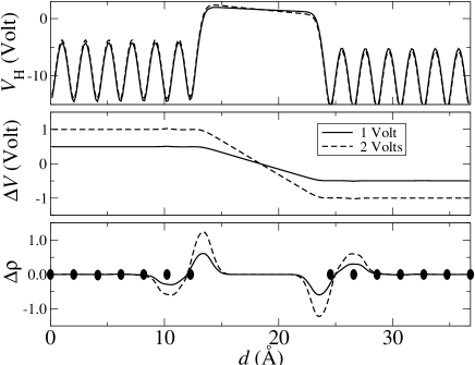
Figure 4: a) Planar average of the Hartree potential $V_{\mathrm{H}}$ for an infinite parallel-plate capacitor. b) Difference between the planar average of the Hartree potential at a given bias and that at zero bias $\Delta V$. c) Difference $\Delta\rho$ between of the planar average of the charge density along the direction of the transport for a given bias and that at zero bias. The dots indicates the position of gold planes.

The quantities shown in the picture are those expected from the classical physics of a parallel plate capacitor. In the leads the electrostatic potential shows oscillations with a period corresponding to that of the separation between the gold planes, but with a constant average. In contrast in the vacuum region the potential is much higher, since there are no contributions from the nuclei, but it is uniform. If we eliminate the oscillations, by subtracting the zero bias potential from that obtained at finite bias (figure 4b), we obtain a constant potential profile in the leads and a linear drop in the vacuum region. Finally the macroscopic average of the charge density shows charge accumulation on the surfaces of the capacitor and local charge neutrality in the leads region as expected from a capacitor.

III.2 Gold nanowires

Metallic quantum point contacts (PCs) present conductance quantization at room temperature ruitenbeek a property that has been predicted theoretically for many yearsGF4 . Recently, Rodrigues et al. have shown that in a point contact the crystallographic orientation of the atomic tips forming the junction plays an important rôle in determining transport properties Rodriguez . Therefore, a realistic theoretical description of the electronic transport in PCs must take into consideration the atomistic aspects of the problem.

As an example we have performed calculations for a [100]-oriented gold quantum point contact (see inset of figure 5). A single gold atom is trapped at its equilibrium position between two [100] fcc pyramids. This is the expected configuration for such a specific crystal orientation, and the configuration likely to form in breaking junction experiments for small elongation of the junction. This has been confirmed by atomic resolution TEM images taka ; ugarte . In this case we have used LDA and a single zeta basis set for $s$, $p$ and $d$ orbitals. The unit cell of the extended molecule now contains 141 atoms (seven planes of the leads are included) and we consider periodic boundary conditions with 16 $k$-points in the 2-D Brillouin zone.

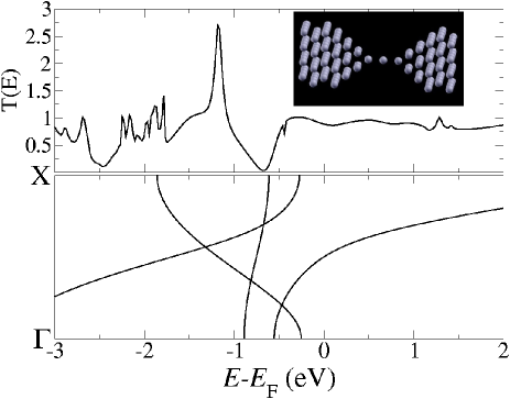
Figure 5: The transmission coefficient as a function of energy (upper panel) for a gold atomic point contact sandwiched between two gold tips oriented along the [100] direction. In the lower panel the bandstructure for a monoatomic gold chain with lattice constant equal to the Au-Au separation in bulk gold. The inset shows a ball-and-stick representation of the atomic positions of the PC (the extended molecule).

In figure 5 we present the zero-bias transmission coefficient as a function of energy. Recalling that the linear response conductance is simply $G=2e^{2}/h\>T(E_{\mathrm{F}})$ (in this case we have complete spin-degeneracy) our calculation shows one quantum conductance for this point contact. Interestingly the transmission coefficient is a rather smooth function $T\sim 1$ for a rather broad energy range around $E_{\mathrm{F}}$. This means that the $G=2e^{2}/h$ result is stable against the fluctuations of the position of the Fermi level, which may be encountered experimentally.

The large plateau at $T\sim 1$ indicates the presence of a single conductance channel for energies around and above $E_{\mathrm{F}}$. This is expected from the bandstructure of a straight monoatomic gold chain with lattice parameter equal to the Au-Au separation in bulk gold (see figure 5b), which presents only one $s$ band for such energy range. Therefore we conclude that the transport at the Fermi level is dominated by a single low-scattering $s$ channel. Notably for energies 1 eV below $E_{\mathrm{F}}$ the transmission coefficient shows values exceeding one, which are due to contributions from $d$ orbitals. In gold mono-atomic chains these are substantially closer to $E_{\mathrm{F}}$ than in bulk gold and participate to the transport. These results are in good agreement with previously reported calculations landman ; rego_rocha and experimental data ruitenbeek ; taka ; RodriguezLett . Additional examples of Smeagol’s calculations for PCs carried out by the authors can be found elsewhere in the literature vic1 ; vic2 .

III.3 Molecular spin-valves

The study of the $I$-$V$ characteristics of magnetic systems at the nanoscale is one of Smeagol’s main goals. The most typical among spin devices is the magnetic spin-valve, which is obtained by sandwiching a non-magnetic spacer between two magnetic contacts. The direction of the magnetization in the two contacts can be arbitrarily changed by applying a magnetic field. The device then switches from a low resistance state, when the magnetization vectors in the leads are parallel to each other, to a high resistance state when the alignment of the magnetizations is antiparallel. This is the giant magnetoresistance effect GMR1 ; GMR2 , which is at the foundation of modern hard-disk reading technology.

Traditional spin-valves use either metals or inorganic insulators as spacers. However a recent series of experiments have shown that organic molecules can serve the same purpose and a rather large GMR can be found bruce ; Aws1 ; Shi ; Dediu ; Ralph . These experiments could lead to integrating the functionalities of molecules with spin-systems, and therefore have the potential to merge together the fields of spin- and molecular-electronics.

The calculation of the transport properties of molecular spin-valves is a tough theoretical problem. It involves the computation of accurate electronic structures for magnetic surfaces, the charging properties of molecules, and the knowledge of the actual atomic positions. In a recent paper Smeagol2 we have demonstrated that molecules can efficiently be employed in spin-valves. Moreover we have shown that $\pi$-conjugated conducting molecules produce larger GMR then their insulating counterparts. Most of the effect is due to the orbital selectivity of the molecule/metal bonding, which in transition metals translates to a spin-selectivity. Here we further expand this concept and we demonstrate that the GMR can be tuned by molecular end-group engineering.

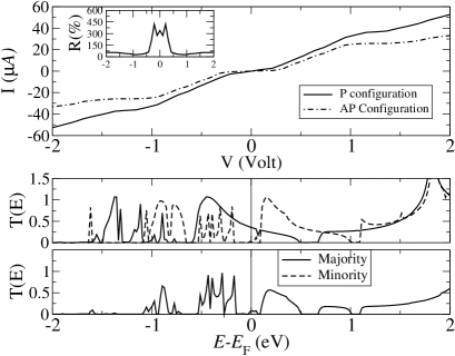
Figure 6: Transport properties for a 1,4-phenyl molecule attached to Ni (100) surfaces through a S group. The top panel shows the $I$-$V$ characteristics for both the parallel and antiparallel alignment of the leads and the inset the corresponding GMR ratio. The lower panel is the transmission coefficient at zero bias as a function of energy. Because of spin-symmetry, in the antiparallel case we plot only the majority spin.

The system under investigation is a 1,4-phenyl molecule attached to two fcc Ni surfaces oriented along the (001) direction. The molecules are attached to the Ni hollow site through a thiol-like group where we use S, Se and Te as anchoring atoms. We consider collinear spin only and investigate the $I$-$V$ characteristic assuming the magnetization vectors in the current/voltage contacts to be either parallel (P) or antiparallel (AP) to each other. The size of the GMR effect is expressed by the GMR ratio $R_{\mathrm{MR}}$, which is defined as $R_{\mathrm{MR}}=(I_{\mathrm{P}}-I_{\mathrm{AP}})/I_{\mathrm{AP}}$, with $I_{\mathrm{P}}$ ($I_{\mathrm{AP}}$) the current in the parallel (antiparallel) state. At zero bias, when all the currents vanish, we replace them with the conductances.

We construct the unit cell of the extended molecule to include four Ni atomic planes on each side, for a total of forty Ni atoms. The basis set is critical and a single zeta for all the orbitals is not sufficient. Therefore we have used single zeta for H, C and S $s$ orbitals, double zeta for Ni $s$, $p$ and $d$, and double zeta polarized for C and S $p$ orbitals. This basis gives us a Hamiltonian with over a thousand degrees of freedom. Finally the charge density is obtained by integrating the Green’s function over 50 imaginary and 600 real energies.

In figures 6, 7 and 8 we present the $I$-$V$ characteristics, the zero bias transmission coefficient as a function of energy, and the GMR ratio as a function of bias for the three anchoring situations (S, Se, Te). Clearly all the three cases show a large GMR, particularly for small biases. Interestingly the maximum GMR increases when going from S to Se to Te, and this is correlated with a general reduction of the total transmission and consequently of the current. Such a reduction is more pronounced in the case of antiparallel alignment of the leads and this gives rise to the increase in GMR. The origin of the drastic reduction of the transmission when changing the anchoring groups has to be found in the different bonding structure. Since S, Se and Te all belong to the same row of the periodic table, the orbital nature of the bonding to the Ni surface is left unchanged, and so are the generic features of the transmission coefficient. However the bond distance goes from 1.28Å to 1.48Å to 1.77Å when going from S to Se to Te. This large increase in the bond distance is responsible for the reduction in transmission.

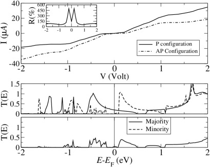
Figure 7: Transport properties for a 1,4-phenyl molecule attached to Ni (100) surfaces through a Se group. The top panel shows the $I$-$V$ characteristics for both the parallel and antiparallel alignment of the leads and the inset the corresponding GMR ratio. The lower panel is the transmission coefficient at zero bias as a function of energy. Because of spin-symmetry, in the antiparallel case we plot only the majority spin.

The most relevant features of the transmission coefficient can be understood in terms of tunneling through a single molecular state Smeagol2 . If we define $t^{\uparrow}(E)$ ($t^{\downarrow}(E)$) as the majority (minority) spin hopping integral from one of the leads to the molecular state, then the total transmission coefficient through the entire device in the parallel alignment will be simply $T=T^{\uparrow\uparrow}+T^{\downarrow\downarrow}=(t^{\uparrow})^{2}+(t^{\downarrow})^{2}$. Here the total transmission coefficient for majority (minority) spin is $T^{\uparrow\uparrow}=(t^{\uparrow})^{2}$ ($T^{\downarrow\downarrow}=(t^{\downarrow})^{2}$). Similarly in the case of antiparallel alignment of the leads we have $T=2T^{{\uparrow\downarrow}}=2T^{\downarrow\uparrow}=2t^{\uparrow}t^{\downarrow}$. In this simple description, which neglects both co-tunnelling and multiple scattering from the contacts, $T^{{\uparrow\downarrow}}(E)$ turns out to be a convolution of the transmission coefficients for the parallel case $T^{\uparrow\downarrow}\propto\sqrt{{T^{\uparrow\uparrow}}T^{\downarrow\downarrow}}$. This type of behavior can be appreciated in figures 6, 7 and 8.

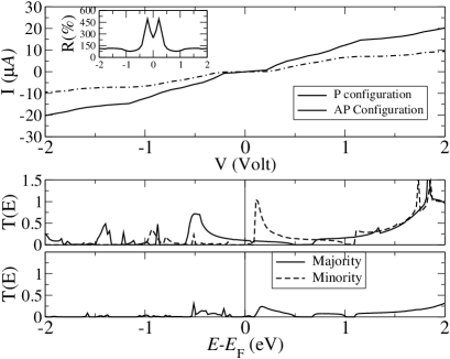
Figure 8: Transport properties for a 1,4-phenyl molecule attached to Ni (100) surfaces through a Te group. The top panel shows the $I$-$V$ characteristics for both the parallel and antiparallel alignment of the leads and the inset the corresponding GMR ratio. The lower panel is the transmission coefficient at zero bias as a function of energy. Because of spin-symmetry, in the antiparallel case we plot only the majority spin.

It is important to note that the large GMR ratio is ultimately due to the low transmission around $E_{\mathrm{F}}$ in the antiparallel case, which originates from the small transmission of the minority spins in the parallel case through the relation $T^{\uparrow\downarrow}(E_{\mathrm{F}})\propto\sqrt{{T^{\uparrow\uparrow}}(E_{\mathrm{F}})T^{\downarrow\downarrow}(E_{\mathrm{F}})}$. This is surprising since the density of states for minority spins at the Fermi level is rather large and one may expect substantial transmission. Moreover $s$-like electrons, which are weakly affected by the spin orientation, generally contribute heavily to the current regardless of the magnetic state of the device. Therefore, what does block the minority spin electrons?

A detailed analysis of the local density of states of the molecule attached to the leads Smeagol2 reveals that the bonding of the molecule to the Ni surface is through Ni $d$ and S $p$ orbitals (the same is valid for Se and Te). The transport is therefore through hybrid Ni $d$-S $p$ states, which in turns are spin-split due to the ferromagnetism of Ni. The crucial point here is that for the minority band these states end up above the Fermi level, and therefore do not contribute to the low bias transport. This is an important observation, since it demonstrates that orbital selectivity in magnetic systems can produce a spin-selectivity, and therefore magnetoresistance type of effects.

III.4 Nickel point contacts

The transport properties of magnetic transition metal point contacts have been the subject of several recent investigations. Technologically these systems are attractive since they can be used as building blocks for read heads in ultra-high density magnetic data storage devices. From a more fundamental point of view they offer the chance to investigate magnetotransport at the atomic level. Magnetic point contacts are effectively spin-valve-like devices, with the spacer now replaced by a narrow constriction where a sharp domain wall can nucleate bruno . Therefore the magnetoresistance can be associated with domain-wall scattering and the MR ratio can be defined earlier.

A simple argument based on the assumption that all the valence electrons can be transmitted with $T\sim 1$ gives an upper bound for the GMR of the order of a few percent (100% in the case of nickel). This however may be rather optimistic since one expects the $d$ electrons to undergo quite some severe scattering. Indeed small values of GMR for Ni point contacts have been measured viret1 . Surprisingly at the same time other groups have measured huge GMR for the same system PC1 ; garcia2001 ; zchopra ; oscar3 . Although mechanical effects can be behind these large values viret2 , the question on whether or not a large GMR of electronic origin can be found in point contacts remains.

Therefore we investigate the zero bias conductance of a four atom long monoatomic Ni chain sandwiched between two Ni (001) surfaces (see figure 9). This is an extreme situation rarely found in actual break junctions Bahn . However an abrupt domain wall (one atomic spacing long) in a monoatomic chain is the smallest domain wall possible, and it is expected to show the larger GMR. For this reason our calculations represent an upper bound on the GMR obtainable in Ni only devices, and they also serve also as a test of the Smeagol capability for dealing with non-collinear spin.

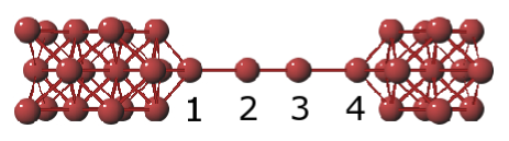
Figure 9: Schematic representation of the Ni point contact simulated. In the symmetric case the domain wall is located between the second and the third atom, while in the asymmetric it is placed between the third and the fourth. The direction of the current is from 1 to 4 for positive bias.

In this calculation we use a double zeta basis set for $s$, $p$ and $d$ orbitals and consider finite leads (no periodic boundary conditions are applied) with either four or five atoms in the cross section. We then investigate two possible situations. In the first one we place the domain wall symmetrically with respect to the leads, i.e. between the second and the third atom of the chain. In the second (asymmetric) the domain wall is positioned between the third and the fourth atom. Furthermore we perform spin-collinear and spin-non-collinear calculations for both cases. Interestingly all our non-collinear calculations always converge to a final collinear solution. This confirms expectations based on simple $s$-$d$ model Maria , suggesting that the strong exchange coupling between the conduction electrons and those responsible for the ferromagnetism, stabilize the collinear state if the magnetization vectors of the leads are collinear.

In figure 10 we present the transmission coefficient as a function of the energy for both the symmetric and asymmetric case and the parallel state. For collinear calculations the contributions from majority and minority spins are plotted separately, while we have only one transmission coefficient in the non-collinear case. Clearly in all cases the non-collinear solution agrees closely with the collinear one, i.e. $T_{\mathrm{collinear}}^{\uparrow}+T_{\mathrm{collinear}}^{\downarrow}=T_{\mathrm{non-collinear}}$. This is expected since the final magnetic arrangement of the non-collinear calculation is actually collinear, and it is a good test for our computational scheme.

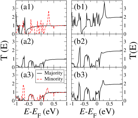
Figure 10: Transmission coefficient as a function of energy for the nickel quantum point contacts of figure 9. The right-hand side panels (a) are for collinear calculations and the left-hand-side (b) are for non-collinear; (1) parallel state, (2) antiparallel with symmetric domain wall, (3) antiparallel with asymmetric domain wall. Note that in the non-collinear case we do not distinguish between majority and minority spins. In panel (a2) majority and minority spins are degenerate.

Turning our attention to the features of the transmission coefficient it is evident that at the Fermi level $T$ in the parallel state is larger than that in the antiparallel. This difference however is not large and the GMR ratio is about 60% with little difference between the symmetric and asymmetric domain wall. This is mainly due to the much higher transmission of the un-polarized $s$ electrons compared with that of the $d$. Note that the conductance approaches $2e^{2}/h$ for energies approximately 0.5 eV above the Fermi level. For such energies in fact no $d$ electrons contribute to the density of states of both the spin sub-bands, and only $s$ electrons are left. These are then transmitted with $T\sim 1$ as in the case of Au chains investigated previously.

The crucial point is that the contribution of the $s$ electrons is also large at the Fermi level. This results in a poorly spin-polarized current at low bias and consequently in a small GMR, in agreement with other calculations mertig ; palacios . In conclusion our finding rules against the possibility of large GMR from electronic origin in Ni point contacts. However the presence of non-magnetic contamination (for example oxygen) may change this picture radically.

III.5 H₂ molecules joining platinum electrodes

The aim of this section is to show how strongly the transmission coefficients may depend on the leads cross section, whenever $d$ electrons are close to $E_{\mathrm{F}}$. As an example, we present results for the H₂ molecule sandwiched between fcc Pt(001) leads, and compare leads of different sections with extended leads. These are obtained by applying periodic boundary conditions and a sampling over the $k$-points along the direction orthogonal to that of transport.

The conductance of an H₂ molecule sandwiched between platinum electrodes has been extensively studied smit ; cuevas ; garcia-pala ; thygesen ; vic1 . Experimentally smit it has been found that the inclusion of hydrogen gas into the vacuum chamber produces a dramatic change in the conductance histograms of platinum, which change from a structure with a broad peak at 1.5 $G_{0}$ to a structure with a sharp peak at 1 $G_{0}$. This resonance has been attributed to the conductance through a single molecule, which bridges both leads lying parallel to the current flow. This explanation has been confirmed by theoretical calculations cuevas ; thygesen ; vic1 .

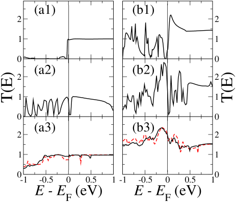
Figure 11: Transmission coefficients for an H₂ molecule sandwiched between fcc platinum leads near the equilibrium distances ($\sim$ 9.5 and 11 Å). The left hand side (a) corresponds to the configuration where the molecule lies parallel to the current flow and the right hand side (b) to the configuration where the molecule lies perpendicular. The leads are made of alternating slabs of 4-5 atoms (1) and 9-12 atoms (2) without periodic boundary conditions along the perpendicular directions ($xy$), and 9-9 atoms with periodic boundary conditions along $xy$ (3). In the last case the dashed and continuous lines have been obtained with 4 and 12 $k$ points, respectively.

In our calculations the H₂ molecules is located either parallel or perpendicular to the current flow. A detailed description of the geometric configuration and the results can also be found in reference [vic1, ]. We use a double zeta polarized basis set for platinum $s$, $p$ and $d$ orbital, a double zeta for the hydrogen $s$ electrons and the LDA functional. As a first step we employ finite cross section leads along the transversal directions, composed of alternated planes containing 4 and 5 atoms each. The resulting transmission coefficients show many peaks and gaps throughout all the energy range and particularly sharp variations around the Fermi energy, as can be seen in figures 11 (a1) and (b1). When thicker slabs composed of alternating planes of 9 and 12 atoms are employed the results do not improve and the large oscillations still remain, as shown in figures 11 (a2) and (b2). It is apparent from these figures that while $T(E)$ shows a long plateau at positive energies, it presents strong oscillations at the Fermi energy and, therefore, it is uncertain to infer the conductance of the junction from $T(E_{\mathrm{F}}$).

This is in stark contrast with the case of gold, where the $d$-levels lie below $E_{\mathrm{F}}$, and $T(E)$ is smooth regardless of the size of the leads cross section. For platinum the presence of $d$-states at the Fermi energy opens minibands and minigaps, which translate into strong oscillations in $T(E\sim E_{\mathrm{F}})$. These minibands and minigaps arise from interference effects of the $d$-states along the transverse direction. Consequently, oscillations in $T(E)$ should disappear when bulk electrodes are used. Indeed, this is what we find when slabs made of 3$\times$3 atomic planes and periodic boundary conditions are employed, as shown in figures 11 (a3) and (b3). We moreover show how $T(E)$ converges when the number of transverse $k$ points is increased from 4 to 12. Although some small variations and peaks still remain when 4 $k$ points are used, the transmission at the Fermi level is essentially converged. Note that the parallel case has $T\sim 1$ for a long range of energies around $E_{\mathrm{F}}$, which remains essentially unperturbed for small variations of the coordinates or the distance between the electrodes. This explains the sharp peak observed in the experimental conductance histograms smit .

In view of the above calculations we can therefore conclude that the use of bulk electrodes, characterized by periodic boundary conditions along the perpendicular directions and $k$ points, is mandatory in order to avoid oscillations in the transmission coefficients. Otherwise the presence of strong variations and minigaps can give unphysical solutions for systems with open $d$ shells.

IV Conclusions

We have presented a description of our newly developed non-equilibrium Green’s function code Smeagol. In the present version Smeagol uses the DFT implementation contained in Siesta as the underlying electronic structure method. However the code has been developed in a modular and general form and can be easily combined with any electronic structure scheme based on localized orbital basis set. The core of Smeagol is our new algorithm for calculating the surface Green’s functions of the leads, which combines generalized singular value decomposition with decimation. This results in an un-precedent numerical stability for a quantum transport code, and in the possibility of drastically reducing the number of degrees of freedom in the leads. In this way large current/voltage probes with complicated electronic structure can be tackled.

We have also presented a selection of results obtained with Smeagol. These range from simple tests for the electrostatics to an analysis of the GMR in molecular spin-valves, and demonstrate the Smeagol’s ability to tackle very different problems.

Appendix A Stable algorithm for the evaluation of the self-energies

A.1 The “$K_{1}$ problem”

The method presented in section II.4 to calculate the leads Green’s functions depends crucially on the fact that the coupling matrix between principal layers $K_{1}=H_{1}-ES_{1}$ is invertible and not ill-defined. However this is not necessarily the case since singularities can be present in $K_{1}$ as the result of poor coupling between PLs or because of symmetry reasons. Note also that since $K_{1}=H_{1}-ES_{1}$ the rank of $K_{1}$ may also depend on the energy $E$.

We now give a few examples illustrating how these singularities arise. Let us consider for the sake of simplicity an orthogonal nearest neighbour tight-binding model with only one $s$-like basis function per atom. In this case $K_{1}=H_{1}$ is independent from the energy. In figure 12 we present four possible cases for which $H_{1}$ is singular.

Figure 12: Four different structures for which $H_{1}$ is singular: (a) lack of bonding, (b) supercell, (c) over-bonding, (d) odd bonding. Each black dot represents an atom and each line a bond. The dashed boxes enclose a principal layer.

In the picture the dots represent the atomic position, the lines the bonds and the dashed boxes enclose a PL. All the bonds are assumed to have the same strength, thus all hopping integrals $\gamma$ are identical.

In the first case (figure 12a) the PL coincides with the primitive unit cell of the system and therefore it is the smaller principal layer that can be constructed. However since every second atom in the cell does not couple with its mirror in the two adjacent cells $H_{1}$ has the form

$$H_{1}=\left(\begin{array}[]{cc}\gamma&0\\ 0&0\\ \end{array}\right)\>$$ (36)

and therefore is singular. This is the case of “lack of bonding” between principal layers. It is the most common case and almost always present when dealing with transition metals, since localized $d$ shells coexist with delocalized $s$ orbitals.

Figure 12b presents a different possibility. Here the PL is a supercell constructed from two unit cells and every atom in the PL couples with atoms located in only one of the two adjacent PLs. In this case

$$H_{1}=\left(\begin{array}[]{cc}0&0\\ \gamma&0\\ \end{array}\right)\>,$$ (37)

which is again singular. Clearly in this specific case one can reduce the principal layer to be the primitive unit cell solving the problem ($H_{1}$ become a scalar $\gamma$). However in a multi-orbital scheme the supercell drawn may be the smallest PL possible and the problem will appear. Again this is a rather typical situation when dealing with transition metals.

The case of “overbonding” is shown in figure 12c. Again the PL coincides with the primitive unit cell, but now every atom in the PL is coupled to all the atoms in the two adjacent PLs. In this case

$$H_{1}=\left(\begin{array}[]{cc}\gamma&\gamma\\ \gamma&\gamma\\ \end{array}\right)\>,$$ (38)

which is not invertible.

Finally the “odd bonding” case is presented in figure 12d. Also in this case the PL coincides with the primitive unit cell, however the upper atom in the cell is coupled only to atoms in the right nearest neighbour principal layer. The $H_{1}$ matrix is then (we label as “1” the upper atom in the cell)

$$H_{1}=\left(\begin{array}[]{cc}0&\gamma\\ 0&\gamma\\ \end{array}\right)\>,$$ (39)

i.e. it is singular. Clearly the above categorization is basis dependent, since one can always find a unitary rotation transforming a generic $H_{1}$ in a new matrix of the form of equation (39).

A.2 Finding the singularities of $K_{1}$

We now present the first step of a scheme for regularizing $K_{1}$, and indeed the whole Hamiltonian and overlap matrix, by removing their singularities. In the cases of “lack of bonding”, “supercell” and “odd bonding” presented in the previous section the singularities of $K_{1}=H_{1}$ were well defined since an entire column was zero. However more generally, and in particular in the case of multiple zetas basis set, $K_{1}$ is singular without having such a simple structure (for instance as in the “overbonding” case). This is the most typical situation and a method for identifying the singularities is needed.

The ultimate goal is to perform a unitary transformation of both ${\cal H}$ and ${\cal S}$ in such a way that the off-diagonal blocks of the leads Hamiltonian and overlap matrix ($H_{1}$ and $S_{1}$) assume the form

$$\begin{array}[]{cc}&\scriptstyle{N-R}\ \ \scriptstyle{R}\\ \scriptstyle{N}&[\>0\>\>,\>\>A\>]\end{array}=\left(\begin{array}[]{cccccc}0&0&\cdots&A_{1,N-R+1}&\cdots&A_{1,N}\\ 0&0&\cdots&A_{2,N-R+1}&\cdots&A_{2,N}\\ 0&0&\cdots&A_{3,N-R+1}&\cdots&A_{3,N}\\ \vdots&\vdots&\vdots&\vdots&\vdots&\vdots\\ 0&0&\cdots&A_{N,N-R+1}&\cdots&A_{N,N}\\ \end{array}\right)\>,$$ (40)

i.e. they are $N\times N$ block matrices of rank $R$, whose first $N-R$ columns vanish. In this form the problem is re-conducted to the problem of “odd bonding” presented in the previous section.

This can be achieved by performing a generalized singular value decomposition (GSVD) lapack . The idea is that a pair of $N\times N$ matrices, in this case $H_{1}$ and $S_{1}$, can be written in the following form

$$H_{1}=U\Lambda_{1}\left[0,W\right]Q^{\dagger},$$ (41)

$$S_{1}=V\Lambda_{2}\left[0,W\right]Q^{\dagger},$$ (42)

with $U$, $V$ and $Q$ unitary $N\times N$ matrices and $W$ being a $R\times R$ non-singular triangular matrix where $R$ is the rank of the $2N\times N$ matrix $\left[\begin{array}[]{c}H_{1}\\ S_{1}\end{array}\right]$ ($R\leq N$). The matrices $\Lambda_{1}$ and $\Lambda_{2}$ are defined as follows:

$$\Lambda_{1}=\begin{array}[]{cc}&\scriptstyle{K}\ \ \scriptstyle{L}\\ \begin{array}[]{r}\scriptstyle{K}\\ \scriptstyle{L}\\ \scriptstyle{N-K-L}\end{array}&\left(\begin{array}[]{cc}I_{K}&0\\ 0&C\\ 0&0\end{array}\right)\end{array},$$ (43)

$$\Lambda_{2}=\begin{array}[]{cc}&\scriptstyle{K}\ \ \scriptstyle{L}\\ \begin{array}[]{r}\scriptstyle{L}\\ \scriptstyle{N-L}\end{array}&\left(\begin{array}[]{cc}0&C^{\prime}\\ 0&0\end{array}\right)\end{array}$$ (44)

where $L$ is the rank of $S_{1}$, $K+L=R$, $I_{K}$ is the $K\times K$ unit matrix and $C$ and $C^{\prime}$ are matrices to determine.

Clearly the two matrices $H_{1}$ and $S_{1}$ have the two common generators $W$ and $Q$. Then, one can perform a unitary transformation of both $H_{1}$ and $S_{1}$ by using $Q$, obtaining

$$H_{1}^{Q}=Q^{\dagger}H_{1}Q=Q^{\dagger}U\Lambda_{1}\left[0,W\right]=\begin{array}[]{rc}&\scriptstyle{N-R}\ \ \ \scriptstyle{R}\\ \scriptstyle{N}&\left[\begin{array}[]{ccc}0&,&\bar{H}_{1}\end{array}\right]\end{array}$$ (48)

$$S_{1}^{Q}=Q^{\dagger}S_{1}Q=Q^{\dagger}V\Lambda_{2}\left[0,W\right]=\begin{array}[]{cc}&\scriptstyle{N-R}\ \ \ \scriptstyle{R}\\ \scriptstyle{N}&\left[\begin{array}[]{ccc}0&,&\bar{S}_{1}\end{array}\right].\end{array}$$ (52)

Here $\bar{H}_{1}$ and $\bar{S}_{1}$ are the $N\times R$ non-vanishing blocks of the GSVD transformed matrices $H_{1}$ and $S_{1}$ respectively.

In an analogous way the same transformation for $H_{1}^{\dagger}$, $S_{1}^{\dagger}$, $H_{0}$ and $S_{0}$ leads to

$${H^{Q}_{1}}^{\dagger}=Q^{\dagger}H_{1}^{\dagger}Q=\begin{array}[]{cc}&\scriptstyle{N}\\ \begin{array}[]{c}\scriptstyle{N-R}\\ \scriptstyle{R}\end{array}&\left[\begin{array}[]{c}0\\ \bar{H}_{1}^{\dagger}\end{array}\right]\end{array}$$ (59)

$${S^{Q}_{1}}^{\dagger}=Q^{\dagger}S_{1}^{\dagger}Q=\begin{array}[]{cc}&\scriptstyle{N}\\ \begin{array}[]{c}\scriptstyle{N-R}\\ \scriptstyle{R}\end{array}&\left[\begin{array}[]{c}0\\ \bar{S}_{1}^{\dagger}\end{array}\right]\end{array}$$ (66)

$$H_{0}^{Q}=Q^{\dagger}H_{0}Q\>,$$ (67)

$$S_{0}^{Q}=Q^{\dagger}S_{0}Q\>,$$ (68)

where the transformed matrices $H_{0}^{Q}$ and $S_{0}^{Q}$ are not necessarily in the form of equation (40).

We are now in the position of writing the final unitary transformations for the total (infinite) Hamiltonian ${\cal H}$ and overlap ${\cal S}$ matrices describing the whole system (leads plus extended molecule). These are given by ${\cal Q}^{\dagger}{\cal HQ}$ and ${\cal Q}^{\dagger}{\cal SQ}$ with the infinite matrix ${\cal Q}$ defined as

$${\cal Q}=\left(\begin{array}[]{ccccccccc}\ddots&.&.&.&.&.&.&.&\\ .&0&Q&0&.&.&.&.&.\\ .&.&0&Q&0&.&.&.&.\\ .&.&.&0&I_{\mathrm{M}}&0&.&.&.\\ .&.&.&.&0&Q&0&.&.\\ .&.&.&.&.&0&Q&0&.\\ .&.&.&.&.&.&.&.&\ddots\\ \end{array}\right)\;,$$ (69)

where $I_{\mathrm{M}}$ is the $M\times M$ unit matrix. Note that this unitary transformation rotates all the $H_{1}$ matrices (the $S_{1}$ matrices in the case of ${\cal S}$), but it leaves $H_{\mathrm{M}}$ ($S_{\mathrm{M}}$) unchanged. Finally the matrices coupling the extended molecule to the leads transform as following

$$\begin{array}[]{l}H_{\mathrm{LM}}^{Q}\>\rightarrow\>Q^{\dagger}H_{\mathrm{LM}}\>,\\ H_{\mathrm{ML}}^{Q}\>\rightarrow\>H_{\mathrm{ML}}Q\>,\\ H_{\mathrm{RM}}^{Q}\>\rightarrow\>Q^{\dagger}H_{\mathrm{RM}}\>,\\ H_{\mathrm{MR}}^{Q}\>\rightarrow\>H_{\mathrm{MR}}Q\;,\\ \end{array}$$ (70)

and so do the corresponding matrices of ${\cal S}$.

A.3 Solution of the “$K^{1}$ problem”

Now that both ${\cal H}$ and ${\cal S}$ have been written in a convenient form we can efficiently renormalize them out. The key observation is that the two (infinite) blocks describing the leads have now the following structure (the ${\cal S}$ matrix has an analogous structure and it is not shown here explicitly)

$${\cal H}_{\mathrm{L/R}}^{Q}=\left(\begin{array}[]{ccccc}\ddots&\vdots&\vdots&\vdots&\\ \cdots&Q^{\dagger}{H}_{0}Q&Q^{\dagger}{H}_{1}Q&0&\cdots\\ \cdots&Q^{\dagger}{H}_{-1}Q&Q^{\dagger}{H}_{0}Q&Q^{\dagger}{H}_{1}Q&\cdots\\ \cdots&0&Q^{\dagger}{H}_{-1}Q&Q^{\dagger}{H}_{0}Q&\cdots\\ &\vdots&\vdots&\vdots&\ddots\end{array}\right)=\left(\begin{array}[]{ccccc}\ddots&\vdots&\vdots&\vdots&\\ \cdots&Q^{\dagger}{H}_{0}Q&\left[\begin{array}[]{cc}0&\bar{H}_{1}\\ \end{array}\right]&0&\cdots\\ \cdots&\left[\begin{array}[]{c}0\\ \bar{H}_{1}^{\dagger}\end{array}\right]&\left(\begin{array}[]{cc}C&B\\ B^{\dagger}&D\end{array}\right)&\left[\begin{array}[]{cc}0&\bar{H}_{1}\\ \end{array}\right]&\cdots\\ \cdots&0&\left[\begin{array}[]{c}0\\ \bar{H}_{1}^{\dagger}\end{array}\right]&\left(\begin{array}[]{cc}C&B\\ B^{\dagger}&D\end{array}\right)&\cdots\\ &\vdots&\vdots&\vdots&\ddots\end{array}\right)\>,$$ (71)

where the matrices $D$, $B$ and $C$ are respectively $R\times R$, $N\times(N-R)$ and $(N-R)\times(N-R)$.

Note that the degrees of freedom (orbitals) contained in the block $C$ of the matrix $H_{0}^{Q}=Q^{\dagger}{H}_{0}Q$ couple to those of only one of the two adjacent PLs. This situation is the generalization to a multi-orbital non-orthogonal tight-binding model of the “odd bonding” case discussed at the beginning of this appendix (figure 12d). These degrees of freedom are somehow redundant and they will be eliminated. We therefore proceed with performing Gaussian elimination rgf (also known as “decimation”) of all the degrees of freedom associated to all the blocks $C$.

The idea is that the Schrödinger equation ${\cal Q}^{\dagger}[{\cal H}-E{\cal S}]{\cal Q}\Psi=0$ can be re-arranged in such a way that a subset of degrees of freedom (in this case those associated to orbitals in a PL that couple only to one adjacent PL) do not appear explicitly. The procedure is recursive. Let us suppose we wish to eliminate the $l$-th row and column of the matrix ${\cal K}^{Q}={\cal Q}^{\dagger}[{\cal H}-E{\cal S}]{\cal Q}$. This can be done by re-arranging the remaining matrix elements according to

$${{\cal K}^{Q}}^{(1)}_{ij}={{\cal K}^{Q}}_{ij}-\frac{{{\cal K}^{Q}}_{il}{{\cal K}^{Q}}_{lj}}{{{\cal K}^{Q}}_{ll}}\>.$$ (72)

The dimension of the resulting new matrix ${{\cal K}^{Q}}^{(1)}$ (“1” indicates that one decimation has been performed) is reduced by one with respect to the original ${\cal K}^{Q}$. This procedure is then repeated and after $r$ decimations we obtain a matrix

$${{\cal K}^{Q}}^{(r)}_{ij}={{\cal K}^{Q}}^{(r)}_{ij}-\frac{{{\cal K}^{Q}}^{(r-1)}_{il}{{\cal K}^{Q}}^{(r-1)}_{lj}}{{{\cal K}^{Q}}^{(r-1)}_{ll}}\;.$$ (73)

Let us now decimate all the matrix elements contained in all the sub-matrices $C$. We obtain a new tridiagonal matrix ${{\cal K}^{Q}}^{(\infty)}$ (“$\infty$” means that an infinite number of decimations have been performed) of the form

$${{\cal K}^{Q}}^{(\infty)}=\left(\begin{array}[]{ccccccccccc}.&.&.&.&.&.&.&.&.&.&\\ 0&\Theta^{\dagger}&\Delta&\Theta&0&.&.&.&.&.&.\\ .&0&\Theta^{\dagger}&\Delta&T_{1}&0&.&.&.&.&.\\ .&.&0&T_{1}^{\dagger}&D_{1}&K_{\mathrm{LM}}^{Q}&0&.&.&.&.\\ .&.&.&0&K_{\mathrm{ML}}^{Q}&K_{\mathrm{M}}&\Theta_{\mathrm{MR}}&0&.&.&.\\ .&.&.&.&0&\Theta_{\mathrm{RM}}&D_{2}&\Theta&0&.&.\\ .&.&.&.&.&0&\Theta^{\dagger}&\Delta&\Theta&0&.\\ .&.&.&.&.&.&0&\Theta^{\dagger}&\Delta&\Theta&0\\ .&.&.&.&.&.&.&.&.&.&.\\ \end{array}\right)\;,$$ (74)

where $K_{\mathrm{LM}}^{Q}=H_{\mathrm{LM}}^{Q}-ES_{\mathrm{LM}}^{Q}$, $K_{\mathrm{ML}}^{Q}=H_{\mathrm{ML}}^{Q}-ES_{\mathrm{ML}}^{Q}$ and $K_{\mathrm{M}}=H_{\mathrm{M}}-ES_{\mathrm{M}}$. The crucial point is that the new matrix ${\cal K}^{Q(\infty)}$ is still in the desired tridiagonal form, but now the coupling matrices between principal layers $\Theta$ are not singular. These are now $R\times R$ matrices obtained from the decimation of the non-coupled degrees of freedom of the matrices $K_{1}^{Q}$ (the $C$ blocks). Moreover the elimination of degrees of freedom achieved with the decimation scheme is carried out only in the leads. The electronic structure of these is not updated during the self-consistent procedure for evaluating the Green’s function, and therefore the information regarding the decimated degrees of freedom are not necessary. In contrast the degrees of freedom of the scattering region are not affected by the decimation or the rotation. Therefore the matrix $K_{\mathrm{M}}$ is unaffected by the decimation.

In the decimated matrix ${{\cal K}^{Q}}^{(\infty)}$ new terms appear ($D_{1}$, $D_{2}$, $T_{1}$ and $\Theta_{\mathrm{MR}}$). These arise from the specific structure of the starting matrix ${\cal Q}^{\dagger}[{\cal H}-E{\cal S}]{\cal Q}$ and from the fact that the complete system (leads plus scattering region) is not periodic. In fact assuming that $j$ is the last principal layer of the left-hand side lead and $l$ is the first layer of right-hand side lead, the decimation is carried out up to $j-1$ to the left and starts from $l$ to the right of the scattering region. This allows us to preserve the tridiagonal form of ${\cal K}$ and at the same time to leave $K_{\mathrm{M}}$ unchanged. A schematic picture of the decimation strategy is illustrated in figure 13.

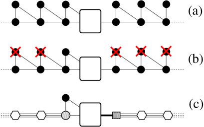
Figure 13: Schematic representation of the decimation strategy for the rotated ${\cal K}$ matrix ${\cal K}^{Q}$. Every symbol (dots, boxes ..) represents a collection of degrees of freedom (a matrix block) and every line the coupling. (a) Original structure after the rotation ${\cal Q}$. In the periodic leads the upper black dots represent the blocks $C$ of the matrix of equation (71). The large white rectangular box represents the scattering region. (b) The degrees of freedom marked with the red crosses are decimated. (c) Final structure after decimation. The new white symbols represent the leads degrees of freedom of the principal layers adjacent to the scattering region as they appear after the decimation.

In practical terms all the blocks of the infinite matrix of equation (74) can be calculated by decimating auxiliary finite matrices. In particular

1. $\Delta$, $\Theta$ and $D_{2}$ are calculated by decimating both the $C$ matrices of the following finite $2N\times 2N$ matrix

   $$\left(\begin{array}[]{cc}\left(\begin{array}[]{cc}C&B\\ B^{\dagger}&D\end{array}\right)&\left[\begin{array}[]{cc}0&\bar{K}_{1}\\ \end{array}\right]\\ \left[\begin{array}[]{c}0\\ {\bar{K}_{1}^{\dagger}}\end{array}\right]&\left(\begin{array}[]{cc}C&B\\ B^{\dagger}&D\end{array}\right)\\ \end{array}\right)\longrightarrow\left(\begin{array}[]{cc}D_{2}&\Theta\\ \Theta^{\dagger}&\Delta\end{array}\right)\>,$$ (75)

   where $\bar{K}_{1}=\bar{H}_{1}-E\bar{S}_{1}$ and

   $$\left(\begin{array}[]{cc}C&B\\ B^{\dagger}&D\end{array}\right)=H_{0}^{Q}-ES_{0}^{Q}\;.$$ (76)

2. $D_{1}$ and $T_{1}$ are calculated by decimating only the upper $C$ matrix of the same finite $2N\times 2N$ matrix

   $$\left(\begin{array}[]{cc}\left(\begin{array}[]{cc}C&B\\ B^{\dagger}&D\end{array}\right)&\left[\begin{array}[]{cc}0&\bar{K}_{1}\\ \end{array}\right]\\ \left[\begin{array}[]{c}0\\ {\bar{K}^{\dagger}_{1}}\end{array}\right]&\left(\begin{array}[]{cc}C&B\\ B^{\dagger}&D\end{array}\right)\\ \end{array}\right)\longrightarrow\left(\begin{array}[]{cc}D_{2}&T_{1}\\ T_{1}^{\dagger}&D_{1}\end{array}\right)\>,$$ (77)

   where $D_{1}$ is $N\times N$, while $T_{1}$ is $R\times N$.

3. $\Theta_{\mathrm{MR}}$ is a $M\times R$ matrix obtained by decimating the $C$ block of the following $(N+M)\times(N+M)$ matrix

   $$\left(\begin{array}[]{cc}0_{\mathrm{M}}&K_{\mathrm{MR}}^{Q}\\ K_{\mathrm{RM}}^{Q}&\left(\begin{array}[]{cc}C&B\\ B^{\dagger}&D\end{array}\right)\\ \end{array}\right)\longrightarrow\left(\begin{array}[]{cc}0_{\mathrm{M}}&\Theta_{\mathrm{MR}}\\ \Theta_{\mathrm{RM}}&D_{2}\end{array}\right)\>,$$ (78)

   where $0_{\mathrm{M}}$ is the $M$-dimensional null matrix.

Finally we are now in the position of calculating the self-energies. These are obtained from the surface Green’s functions for the rotated and decimated leads (specified by the matrices $\Delta$ and $\Theta$) and have the following form

$$\Sigma_{L}=K_{\mathrm{ML}}^{Q}\left(-D_{1}-T_{1}^{\dagger}G_{\mathrm{L}}T_{1}\right)^{-1}K_{\mathrm{LM}}^{Q}$$ (79)

and

$$\Sigma_{R}=\Theta_{\mathrm{MR}}\left[G_{\mathrm{R}}^{-1}-(D_{2}-\Delta)\right]^{-1}\Theta_{\mathrm{RM}}\>.$$ (80)

Clearly our procedure not only regularizes the algorithm for calculating the self-energies, giving it the necessary numerical stability, but also drastically reduces the degrees of freedom (orbitals) needed for solving the transport problem. These go from $N$ (the dimension of the original $H_{1}$ matrix) to $R$ (the rank of $H_{1}$). Usually $R\ll N$ and considerable computational overheads are saved.

Finally it is important to note that usually the rank $R$ of $\left[\begin{array}[]{c}H_{1}\\ S_{1}\end{array}\right]$ is not necessarily the same of that of $\left[\begin{array}[]{c}H_{1}^{\dagger}\\ S_{1}^{\dagger}\end{array}\right]$ ($R^{\prime}$). If $R^{\prime}<R$ the GSVD transformation must be performed over the matrices $H_{1}^{\dagger}$ and $S_{1}^{\dagger}$. The procedure is similar to what described before but the final structure of the matrix ${\cal K}^{Q}$ is somehow different, and so should be the decimation scheme.

Appendix B Theoretical description

B.1 Brief reminder of Keldish formalism

The electronic part of the system we consider is described in a general way by the following Hamiltonian Wag91

$$H(\vec{r}_{1},\vec{r}_{2},t)=H_{0}(\vec{r}_{1},t)\delta(\vec{r}_{1}-\vec{r_{2}})+H_{1}(\vec{r}_{1},\vec{r}_{2})$$ (81)

where $H_{1}$ accounts for the Coulomb interaction among electrons and $H_{0}$ stands for all one-particle pieces of the Hamiltonian,

$$H_{0}(\vec{r},t)=H_{\mathrm{kin}}(\vec{r})+H_{\mathrm{ei}}(\vec{r})+V_{\mathrm{ext}}(\vec{r},t)\;.$$ (82)

$H_{\mathrm{kin}}$ and $H_{\mathrm{ei}}$ are respectively the kinetic energy and the Coulomb interaction between electrons and nuclei, and $V_{\mathrm{ext}}$ is an external electrostatic potentials applied to the system at $t=0$.

The electronic system evolves according to the time-independent Hamiltonian $H(t_{0}=0^{-})$ for all negative times, and uses $t_{0}$ as the synchronization time for all pictures. Moreover we assume that before $V_{\mathrm{ext}}$ is switched on the system of interacting electrons is in thermodynamic equilibrium at a chemical potential $\mu_{0}$. We then prepare the density matrix $\rho$ at $t_{0}$ also. Therefore, expectation values of observables

$$\langle\hat{O}(t)\rangle = Tr\{\rho^{S}(t)\,\hat{O}^{S}(t)\}=Tr\{\rho^{H}(t_{0})\,\hat{O}^{H}(t)\}$$ (83)

$$= \frac{1}{Z}\,Tr\{e^{-\beta\,(H(t_{0})-\mu_{0}\,N)}\,\hat{O}^{H}(t)\}$$

are described in terms of the density matrix of an interacting electron system at equilibrium.

These expectation values may be evaluated by using perturbation theory. Wick’s theorem may be applied only to ensembles of non-interacting electrons. In order to take advantage of it, we must use a non-interacting density matrix such as

$$\rho_{0}(t_{0})=\frac{e^{-\beta\,(H_{0}(t_{0})-\mu_{0}\,N)}}{Z_{0}}$$ (84)

We then define the Hamiltonian in the Schrödinger picture in the Keldish contour of Fig. 14 of the complex $\tau$ plane as follows

$$K^{S}(\tau)=\left\{\begin{array}[]{ll}H^{S}(\tau)&\tau\,\in\,c_{H}\\ H^{S}(0)-\mu_{0}\,N&\tau\,\in\,c_{V}\end{array}\right.$$ (85)

and analogous expressions for its noninteracting and interacting pieces, $K_{0}^{S}(\tau)$ and $K_{1}^{S}(\tau)$. We notice that the time variable is doubled valued along the real axis. We must therefore distinguish whether any real time lies on the upper ($t^{+}$) or lower ($t^{-}$) branch.

Figure 14: Keldish contour $c$ in the complex $\tau$ plane. The imaginary time path is called $c_{1}$ or $c_{V}$ in the text. The segment lying below (above) the real-time axis is called $c_{2}$ ($c_{3}$). The time loop $c_{2}$+$c_{3}$ is called $c_{H}$.

We then define Heisenberg (H) and Dirac (D) pictures in the Keldish contour whereby evolution of operators is provided by

$$\hat{O}^{H}(t) = T_{c}\,\,e^{-i\,\int_{0^{+}}^{0^{-}}\,d\tau^{\prime}\,K^{S}(\tau^{\prime})}\,\hat{O}^{S}(t)=T_{c}\,U(0^{+},0^{-})\,\hat{O}^{S}(t)$$

$$\hat{O}^{D}(t) = T_{c}\,\,e^{-i\,\int_{0^{+}}^{0^{-}}\,d\tau^{\prime}\,K^{S}_{0}(\tau^{\prime})}\,\hat{O}^{S}(t)=T_{c}\,V_{0}(0^{+},0^{-})\,\hat{O}^{S}(t)$$

$$= T_{c}\,\,e^{-i\,\int_{0^{+}}^{0^{-}}\,d\tau^{\prime}\,K^{D}_{1}(\tau^{\prime})}\,\hat{O}^{H}(t)=T_{c}\,V_{1}(0^{+},0^{-})\,\hat{O}^{H}(t)$$

where $T_{c}$ is the time ordering operator on $c$. Expectation values of operators are then given by the statistical averages

$$\langle\hat{O}(t)\rangle=\frac{Z_{0}}{Z}\,Tr\{\rho_{0}\,V_{1}(-i\,\beta,0^{+})\,\hat{O}(t)\}.$$ (86)

which are evaluated in the non-interacting ensemble described by $\rho_{0}$.

The Green function of the system,

$$G(1,2)=\langle T_{c}\,\hat{\psi}(1)\,\hat{\psi}^{\dagger}(2)\rangle$$ (87)

is a tool to compute the physical response of the system. Thus the electron charge and current densities are simply

$$\langle\hat{n}(1)\rangle = -i\,e\,G(1^{+},1^{-})$$ (88)

$$\langle\hat{\vec{\j}}(1)\rangle = -\frac{e\,\hbar}{2\,m}\,\left[\vec{\nabla}_{1}-\vec{\nabla}_{2}+2\,i\,\vec{A}(1)\right]\,G(1^{+},2)|_{2=1^{-}}$$

and depend on the applied the external potential. Here, $\hat{\psi}\,,\hat{\psi}^{\dagger}$ denote creation and annihilation operators, and $(i)=(\vec{r}_{i},t_{i})$.

The Green’s function can be proven to satisfy the following Dyson equation

$$\left[\,i\,\partial_{t_{1}}-H_{0}(1)\,\right]\,G(1,2) = \delta(1,2)+(\Sigma\otimes G)\,(1,2)$$

$$\left[\,-i\,\partial_{t_{2}}-H_{0}(2)\,\right]\,G(1,2) = \delta(1,2)+(G\otimes\Sigma)\,(1,2)$$

where all time variables run through the Keldish contour $c$ and we follow the conventional shorthand

$$(A\otimes B)(1,2)=\int_{c}\,dx_{3}\,dt_{3}A(1,3)\,B(3,2)$$ (89)

B.2 Connection to TDDFT

We now define a fictitious system of non-interacting electrons described by the Hamiltonian Lee01

$$H_{s}(\vec{r},t)=H_{\mathrm{kin}}(\vec{r})+V_{s}(\vec{r},t)$$ (90)

where we assume that $H_{s}$ is constant and that the system is in thermodynamic equilibrium at chemical potential $\mu_{s}$, all for negative times. We also assume that $H_{s}$ may be exactly diagonalized. We do not split a perturbing piece from the Hamiltonian and therefore, Heisenberg and Dirac pictures coincide. We again take $t_{0}$ as the synchronization and density-matrix preparation time. The density matrix

$$\rho_{s}(t_{0})=\frac{e^{-\beta\,(H_{s}(t_{0})-\mu_{s}\,N)}}{Z_{0}}$$ (91)

and the time-evolution operator on the Keldish contour

$$U_{s}(0^{+},0^{-})=T_{c}\,\,e^{-i\,\int_{0^{+}}^{0^{-}}\,d\tau^{\prime}\,K^{S}_{s}(\tau^{\prime})}$$ (92)

completely determine the expectation value of observables of this fictitious system

$$\langle\hat{O}(t)\rangle_{s}=Tr\{\rho^{S}_{s}(t)\,\hat{O}^{S}(t)\}=Tr\{\rho^{H}_{s}(t_{0})\,\hat{O}^{H}(t)\}$$

The Green’s function $G_{s}(1,1^{\prime})$, whose time variables also lie on $c$, satisfies the equation of motion

$$\left[\,i\,\partial_{t_{1}}-H_{s}(1)\,\right]\,G_{s}(1,2) = \delta(1,2)$$

$$\left[\,-i\,\partial_{t_{2}}-H_{s}(2)\,\right]\,G_{s}(1,2) = \delta(1,2)$$ (93)

and provides the physical response of the system

$$n_{s}[V_{s}(1)] = -i\,e\,G_{s}(1^{+},1^{-})$$

$$\vec{\j}_{s}[V_{s}(1)] = -\frac{e\,\hbar}{2\,m}\,\left[\vec{\nabla}_{1}-\vec{\nabla}_{2}+2\,i\,\vec{A}(1)\right]\,G_{s}(1^{+},2)|_{2=1^{-}}$$

We define the action functionals

$$R[V(x)] = i\,\ln\mathrm{Tr}\left[\hat{U}(-i\,\beta,0)\right]$$

$$R_{s}[V_{s}(x)] = i\,\ln\mathrm{Tr}\left[\hat{U}_{s}(-i\,\beta,0)\right]$$ (94)

whose functional derivative with respect to the external potential provides an alternative way to calculate the electronic density. We adjust the potential $V_{s}$ so that the densities of the two systems be equal,

$$\frac{\delta R[V(x)]}{\delta V(x)}=\frac{\delta R[V_{s}(x)]}{\delta V_{s}(x)}=\langle n(x)\rangle$$ (95)

Notice that we do not require that the current densities of the two systems be equal.

We now perform a Legendre transform to find the new actions

$$S[n] = -R[V[n]]+\int dx\,n(x)\,V(x)$$

$$S_{s}[n] = -R_{s}[V_{s}[n]]+\int dx\,n(x)\,V_{s}(x)$$ (96)

such that

$$\frac{\delta S[n(x)]}{\delta n(x)} = V(x)$$

$$\frac{\delta S_{s}[n(x)]}{\delta n(x)} = V_{s}(x)$$ (97)

We define an exchange-correlation functional

$$S_{s}[n]=S[n]+\frac{1}{2}\int\,dx\;[V_{\mathrm{H}}(x)\,n(x)+S_{\mathrm{xc}}[n]]$$ (98)

whose functional derivative with respect to the density provides with a key relationship between the external potential of the actual and fictitious systems,

$$V_{s}(x) = V(x)+V_{\mathrm{H}}(x)+V_{\mathrm{xc}}(x)$$

$$V_{\mathrm{xc}}[n(x)] = \frac{\delta S_{\mathrm{xc}}}{\delta n(x)}$$ (99)

Comparing the equations of motion of $G$ and $G_{s}$, we find an explicit relationship between the Green’s functions

$$G=G_{s}+G_{s}\otimes(\,\Sigma-V_{\mathrm{H}}-V_{\mathrm{xc}}\,)\otimes G$$ (100)

and the Sham-Schlüter equation for the Self-energy

$$G_{s}\otimes(\,V_{\mathrm{H}}+V_{\mathrm{xc}}\,)\otimes G=G_{s}\otimes\Sigma[G]\otimes G$$ (101)

Iterating these equations once means equating both Green’s functions, $G=G_{s}$, which in turn implies approximating $\vec{\j}$ by $\vec{\j}_{s}$. The resulting integral equation for $\Sigma$ has

$$\Sigma[G](1,2)=(\,V_{\mathrm{H}}[n(1)]+V_{\mathrm{xc}}[n(1)]\,)\,\delta(1,2)$$ (102)

as a trivial solution. This simple approximation has the virtue that charge is conserved. This can be seen in two alternative ways. First, the self-energy can be written as a $\Phi[G]$-derivable function. Second, the fictitious system satisfies the continuity equation by construction. Subsequent iterations improve the physical content of $G$, but we have used in our code this lowest-order approximation.

The Green’s function at two different times $G(t,t^{\prime})$ can be viewed as the matrix element $\langle t|G|t^{\prime}\rangle$, sandwiched between two time states of the whole set $\{|t\rangle\}$ of times in the Keldish contour. We split the contour into the three pieces $c_{1},\,c_{2},\,c_{3}$ of Fig. 2, and define the corresponding three time subsets. The Green’s function can then be represented in matrix form as

$$\hat{G}_{s}(t,t^{\prime}) = \left(\begin{array}[]{ccc}G^{11}(t,t^{\prime})&G^{12}(t,t^{\prime})&G^{13}(t,t^{\prime})\\ G^{21}(t,t^{\prime})&G^{22}(t,t^{\prime})&G^{23}(t,t^{\prime})\\ G^{31}(t,t^{\prime})&G^{32}(t,t^{\prime})&G^{33}(t,t^{\prime})\end{array}\right)$$

$$= \left(\begin{array}[]{ccc}G^{c}(t,t^{\prime})&G^{<}(t,t^{\prime})&G^{13}(t,t^{\prime})\\ G^{>}(t,t^{\prime})&G^{ac}(t,t^{\prime})&G^{13}(t,t^{\prime})\\ G^{31}(t,t^{\prime})&G^{31}(t,t^{\prime})&G^{33}(t,t^{\prime})\end{array}\right)$$

The physical response of the system is therefore encapsulated in the lesser Green function,

$$n[V_{s}(1)] = -i\,G_{s}^{<}(1^{+},1^{-})$$

$$\vec{\j}[V_{s}(1)] = -\frac{\hbar}{2\,m}\,\left[\vec{\nabla}_{1}-\vec{\nabla}_{2}+2\,i\,\vec{A}(1)\right]\,G_{s}^{<}(1^{+},2)|_{2=1^{-}}$$

There are only five independent $G^{ij}$ out of the seven matrix elements displayed above. A partial reduction to six matrix elements in the Green’s function is achieved by the non-unitary transformation

$$\check{G}_{s}(t,t^{\prime})=L\,\tau_{3}\,\hat{G}_{s}(t,t^{\prime})\,L^{\dagger}=\left(\begin{array}[]{ccc}G^{\mathrm{R}}&G^{\mathrm{K}}&\sqrt{2}\,G^{13}\\ 0&G^{\mathrm{A}}&0\\ 0&\sqrt{2}\,G^{31}&G^{3}3\end{array}\right)$$

Both matrices satisfy the matrix equations of motion

$$\left[\,i\,\partial_{t_{1}}-H_{s}(1)\,\right]\,\hat{G}_{s}(1,2) = \delta(\vec{r}_{1}-\vec{r}_{2})\,\hat{\delta}(\tau_{1}-\tau_{2})$$

$$\left[\,i\,\partial_{t_{1}}-H_{s}(1)\,\right]\,\check{G}_{s}(1,2) = \delta(\vec{r}_{1}-\vec{r}_{2})\,\check{\delta}(\tau_{1}-\tau_{2})$$

where the time delta functions are defined as

$$\hat{\delta}\,,\check{\delta}=\left(\begin{array}[]{ccc}\delta(t_{1}-t_{2})&0&0\\ 0&\pm\delta(t_{1}-t_{2})&0\\ 0&0&\delta(\tau_{1}-\tau_{2})\end{array}\right)$$ (106)

with the menos (plus) sign corresponding to the hat (check) delta function. We shall drop the “$s$” subindex from now on, since all the discussion that follows is valid only for the ficticious system of non-interacting electrons.

Physical response is customarily written in terms of $G^{\mathrm{R,A}}$ and $G^{<}$. Since there is no linear transformation which allow to group them in one common matrix, one uses Langreth’s rules to find relationships among them.

B.3 Equations of motion in the localized wave function basis

The eigenstates of the system can be obtained by expanding them in the basis of non-orthogonal states, $\Psi(n,\vec{r},t)=\sum_{i,\mu}\,c_{i\>\mu}(n,t)\,\psi_{\mu}(\vec{r}-\vec{R}_{i})$, in terms of which the Schrödinger equation reads

$$\left[i\,S_{i\mu\>j\nu}\,\partial_{t_{1}}-H_{i\mu\>j\nu}(t_{1})\right]\,c_{j\>\nu}(n,t_{1})=0$$ (107)

Alternatively the equation of motion for either check or hat Green functions are

$$\left[\,i\,S_{i\mu\>k\lambda}\,\partial_{t_{1}}-H_{i\mu\>k\lambda}(t_{1})\,\right]\,G_{k\lambda\>j\nu}(t_{1},t_{2})=\delta_{ij}\,\delta_{\mu\nu}\,\hat{\delta}(t_{1}-t_{2})$$

It is advantageous to perform a change of time variables from $t_{1},t_{2}$ to $T=1/2(t_{1}+t_{2}),t=t_{1}-t_{2}$. Then the Green’s functions can be written as

$$G_{i\mu\>j\nu}(t_{1},t_{2})=G_{i\mu\>j\nu}(T,t)=\int\,\frac{dE}{2\,\pi}\,G_{i\mu\>j\nu}(T,E)\,e^{-i\,E\,t}$$

The electron charge and current densities are found from

$$n(\vec{r},T) = \sum_{i\mu\>j\nu}\,n_{i\mu\>j\nu}(\vec{r})\,\rho_{i\mu\>j\nu}(T)$$

$$\vec{\j}(\vec{r},T) = \sum_{i\mu\>j\nu}\,j_{i\mu\>j\nu}(\vec{r})\,\rho_{i\mu\>j\nu}(T)$$ (108)

where we have introduced the density matrix

$$\rho_{i\mu\>j\nu}(T)=\int\,\frac{dE}{2\,\pi\,i}\,G_{i\mu\>j\nu}^{<}(T,E)$$ (109)

and

$$n_{i\mu\>j\nu}(\vec{r}_{1},\vec{r}_{2})=e\,\psi_{\mu}(\vec{r}_{1}-\vec{R}_{i})\,\,\psi_{\nu}(\vec{r}_{2}-\vec{R}_{j})$$

$$\vec{\j}_{i\mu\>j\nu}(\vec{r})=-\frac{i\,e\,\hbar}{2\,m}\left(\vec{\nabla}_{\vec{r}_{1}}-\vec{\nabla}_{\vec{r}_{2}}+2i\,\vec{A}(\vec{r}_{1})\right)\,n_{i\mu\>j\nu}(\vec{r}_{1},\vec{r}_{2})|_{r_{2}=r_{1}}$$

The electric current through a given surface $S$ is obtained by integrating the current density over such surface

$$I = \int_{S}d\vec{S}\cdot\vec{\j}(\vec{r},t_{1})=\sum_{i\mu\>j\nu}\rho_{i\mu\>j\nu}(t_{1})\int_{S}\,d\vec{S}\cdot\vec{\j}_{i\mu\>j\nu}$$ (110)

$$= \sum_{i^{\prime}\mu^{\prime}\>j^{\prime}\nu^{\prime}}\rho_{i^{\prime}\mu^{\prime}\>j^{\prime}\nu^{\prime}}\,H_{i^{\prime}\mu^{\prime}\>j^{\prime}\nu^{\prime}}$$

where only those bonds $(i^{\prime}\mu\>j^{\prime}\nu^{\prime})$ pierced by the surface contribute to the summation.

If the system is in thermodynamic equilibrium, the population of electrons does not depend on time, and follows the Fermi-Dirac distribution function $f(\epsilon)$. Thereby the lesser Green function can be written in terms of the retarded one as

$$G^{<}_{i\mu\>j\nu}(E) = f(E)\,\left[G^{\mathrm{A}}_{i\mu\>j\nu}(E)-G^{\mathrm{R}}_{i\mu\>j\nu}(E)\right]=$$

$$= -2\,i\,f(E)\,\mathrm{Im}\,\left[G^{\mathrm{R}}_{i\mu\>j\nu}(E)\right]=$$

$$= 2\,\pi\,i\,f(E)\,\sum_{n}\,c_{i\mu}(n)\,c_{j\nu}^{*}(n)\,\delta(E-\epsilon_{n})$$

where $\epsilon_{n}$ are the eigenvalues of the Hamiltonian. Therefore, the density matrix can be obtained from the wave function coefficients by just diagonalising the Hamiltonian,

$$\rho_{i\mu\>j\nu} = -\frac{1}{\pi}\int{\mathrm{d}}E\,f(E)\,\mathrm{Im}\,\left[G^{\mathrm{R}}_{i\mu\>j\nu}(E)\right]=$$ (111)

$$= \sum_{n}\,c_{i\mu}(n)\,c_{j\nu}^{*}(n)\,f(\epsilon_{n})$$

B.4 The extended molecule setup

We now wish to partition the Green functions according to the system setup of Fig. 1, where the left and right leads remain in thermodynamic equilibrium defined by $\mu_{\mathrm{L/R}}=E_{\mathrm{F}}\pm e\,V/2$ at all times. The extended molecule is also in thermodynamic equilibrium for times $t<0$. The Hamiltonian for negative times

$${\cal H}(t<0)=h(t)=\left(\begin{array}[]{ccc}{\cal H}_{\mathrm{L}}+eV/2\,{\cal S}_{\mathrm{L}}&0&0\\ 0&H_{\mathrm{M}}&0\\ 0&0&{\cal H}_{\mathrm{R}}-eV/2\>{\cal S}_{\mathrm{R}}\\ \end{array}\right)\>,$$

serves to define the reference equilibrium hat and check Green functions, that satisfy the equations of motion

$$\left[\,i\,S_{i\mu,k\lambda}\,\partial_{t_{1}}-h_{i\mu,k\lambda}(t_{1})\,\right]\,G_{k\lambda,j\nu}(t_{1},t_{2})=\delta_{i,j}\,\delta_{\mu,\nu}\,\hat{\delta}(t_{1}-t_{2})$$

For instance, the equation of motion for the retarded Green function in frequency domain is just

$$\left(\begin{array}[]{ccc}(\epsilon^{+}-eV/2){\cal S}_{\mathrm{L}}-{\cal H}_{\mathrm{L}}&0&0\\ 0&\epsilon^{+}S_{\mathrm{M}}-H_{\mathrm{M}}&0\\ 0&0&(\epsilon^{+}+eV/2){\cal S}_{\mathrm{RM}}-{\cal H}_{\mathrm{RM}}\\ \end{array}\right)\left(\begin{array}[]{ccc}{\cal G}_{\mathrm{L}}^{0\mathrm{R}}&0&0\\ 0&G_{\mathrm{M}}^{0\mathrm{R}}&0\\ 0&0&{\cal G}_{\mathrm{R}}^{0\mathrm{R}}\\ \end{array}\right)=\left(\begin{array}[]{ccc}{\cal I}&0&0\\ 0&I_{\mathrm{M}}&0\\ 0&0&{\cal I}\\ \end{array}\right)\;,$$ (112)

while the lesser Green function is

$${\cal G}^{0<}(E)=\left(\begin{array}[]{ccc}\left({\cal G}_{\mathrm{L}}^{0\mathrm{A}}(E)-{\cal G}_{\mathrm{L}}^{0\mathrm{R}}(E)\right)\,f(E-eV/2)&0&0\\ 0&G_{M}^{0<}(E)&0\\ 0&0&\left({\cal G}_{\mathrm{R}}^{0\mathrm{A}}(E)-{\cal G}_{\mathrm{R}}^{0\mathrm{R}}(E)\right)\,f(E+eV/2)\end{array}\right)$$ (113)

The extended molecule is contacted by the electrodes at time $t=0$, through the Hamiltonian matrix elements

$$V_{ext}=\left(\begin{array}[]{ccc}0&{\cal H}_{\mathrm{LM}}&0\\ {\cal H}_{\mathrm{ML}}&0&{\cal H}_{\mathrm{MR}}\\ 0&{\cal H}_{\mathrm{RM}}&0\\ \end{array}\right)\>F(t),$$ (114)

where $F(t)$ is zero for negative times, and 1 for times larger than a certain characteristic time $\tau_{M}$. The perturbation $V_{ext}$ drives the core of the extended molecule out of equilibrium for positive times, by populating it with a distribution of electrons that does not follow Fermi-Dirac statistics. The distribution function of the non-contacted molecule $g_{M}^{<}(E)$ is completely washed out, but the density-matrix of the system can still be determined from the equations of motion of the lesser and retarded Green functions.

We seek to solve the equations of motion for times $t\gg\tau_{M}$ where all transient effects have vanished. This means, first, that $G^{1,3}=G^{3,1}=0$, so that the matrix hat and check Green functions are block-diagonal; second, that the Hamiltonian is simply ${\cal H}$; and third, that Green functions do not depend on the time variable T.

The retarded Green function is, simply,

$$\left(\begin{array}[]{ccc}(\epsilon^{+}-eV/2)\,{\cal S}_{\mathrm{L}}-{\cal H}_{\mathrm{L}}&\epsilon^{+}{\cal S}_{\mathrm{LM}}-{\cal H}_{\mathrm{LM}}&0\\ \epsilon^{+}{\cal S}_{\mathrm{ML}}-{\cal H}_{\mathrm{ML}}&\epsilon^{+}S_{\mathrm{M}}-H_{\mathrm{M}}&\epsilon^{+}{\cal S}_{\mathrm{MR}}-{\cal H}_{\mathrm{MR}}\\ 0&\epsilon^{+}{\cal S}_{\mathrm{RM}}-{\cal H}_{\mathrm{RM}}&(\epsilon^{+}+eV/2)\,{\cal S}_{\mathrm{R}}-{\cal H}_{\mathrm{R}}\\ \end{array}\right)\left(\begin{array}[]{ccc}{\cal G}_{\mathrm{L}}^{\mathrm{R}}&{\cal G}_{\mathrm{LM}}^{\mathrm{R}}&{\cal G}_{\mathrm{LR}}^{\mathrm{R}}\\ {\cal G}_{\mathrm{ML}}^{\mathrm{R}}&G_{\mathrm{M}}^{\mathrm{R}}&{\cal G}_{\mathrm{MR}}^{\mathrm{R}}\\ {\cal G}_{\mathrm{RL}}^{\mathrm{R}}&{\cal G}_{\mathrm{RM}}^{\mathrm{R}}&{\cal G}_{\mathrm{R}}^{\mathrm{R}}\\ \end{array}\right)=\left(\begin{array}[]{ccc}{\cal I}&0&0\\ 0&I_{\mathrm{M}}&0\\ 0&0&{\cal I}\\ \end{array}\right)\;,$$ (115)

The lesser Green function is better expressed in terms of the retarded and advanced, and the reference equilibrium lesser Green function, by using Langreth’s rules, as

$${\cal G}^{<}={\cal G}^{\mathrm{R}}\,({\cal G}^{0\mathrm{R}})^{-1}\,{\cal G}^{0<}\,({\cal G}^{0\mathrm{A}})^{-1}\,{\cal G}^{\mathrm{A}}$$ (116)

Straightforward matrix algebra then leads to Eqs. (16) and (19).

References

- (1) G. Binnig, H. Rohrer, Ch. Gerber and E. Weibel, Phys. Rev. Lett. 50, 120 (1983).
- (2) P.J. Kuekes, J.R. Heath, and R.S. Williams, US Patent, number 6128214 (Hewlett-Packard), October 2000.
- (3) C.P. Collier, E.W. Wong, M. Belohradsky, F.M. Raymo, J.F. Stoddart, P.J. Kuekes, R.S. Williams and J.R. Heath, Science 285, 391 (1999).
- (4) Y. Huang, X. Duan, Y. Cui, L.J. Lauhon, K.-H. Kim, C.M. Lieber, Science 294, 1313 (2001).
- (5) N. García, M. Muñoz, and Y.-W. Zhao, Phys. Rev. Lett. 82, 2923 (1999).
- (6) J.J. Versluijs, M.A. Bari, and J.M.D. Coey, Phys. Rev. Lett. 87, 026601 (2001).
- (7) P. Qi, O. Vermesh, M. Grecu, A. Javey, Q. Wang, H. Dai, S. Peng and K. Cho, Nano Lett. 3, 347 (2003).
- (8) J.P. Novak, E.S. Show, E.J. Houser, D. Park, J.L. Stepnowski, and R.A. McGill, Appl. Phys. Lett. 83, 4026 (2003).
- (9) F. Patolsky, et al., Proc. Natl. Acad. Sci. USA 101, 14017 (2004).
- (10) Y. Cui, W. Qingqiao, P. Hongkun, and C.M. Lieber, Science 293, 1289 (2001).
- (11) J.P. Heath, M.E. Phelps and L. Hood, Mol. Im. Biol. 5, 312 (2003).
- (12) S. Datta, Electronic Transport in Mesoscopic Systems, Cambridge University Press, Cambridge, UK, 1995.
- (13) H. Haug and A. P. Jauho, Quantum Kinetics in Transport and Optics of Semiconductors, Springer, Berlin, 1996.
- (14) C. Caroli, R. Combescot, P. Nozieres, and D. Saint-James, J. Phys. C: Solid State Phys. 5, 21 (1972).
- (15) J. Ferrer, A. Martín-Rodero, and F. Flores, Phys. Rev. B 38, R10113 (1988).
- (16) N. D. Lang, Phys. Rev. B 36, R8173 (1987).
- (17) N. D. Lang, Phys. Rev. B 52, 5335 (1995).
- (18) M. Di Ventra, S. T. Pantelides, and N. D. Lang, Phys. Rev. Lett. 84, 979 (2000).
- (19) C.W.J. Beenakker, Phys. Rev. B 44, 1646 (1991)
- (20) R. Gebauer and R. Car, Phys. Rev. B 70, 125324 (2004).
- (21) B. Muralidharan, A.W. Ghosh, S.K. Pati and S. Datta, cond-mat/0505375
- (22) S. Sanvito, in Handbook of Computational Nanotechnology, American Scientific Publishers (Stevenson Ranch, California, 2005), also cond-mat/0503445.
- (23) G. Stefanucci and C.-O. Almbladh, Phys. Rev. B 69, 195318 (2004).
- (24) H. Hohenberg and W. Kohn, Phys. Rev. 136, B864 (1964).
- (25) W. Kohn and L.J. Sham, Phys. Rev. 140, A1133 (1965).
- (26) J. Taylor, H. Guo, and J. Wang, Phys. Rev. B 63, 245407 (2001).
- (27) Y. Xue, S. Datta and M.A. Ratner, Chem. Phys. 281, 151 (2002).
- (28) M. Brandbyge, J.-L. Mozos, P. Ordejón, J. Taylor, and K. Stokbro, Phys. Rev. B 65, 165401 (2002).
- (29) J. J. Palacios, A. J. Pérez-Jiménez, E. Louis, E. SanFabián, and J. A. Vergés, Phys. Rev. B 66, 035322 (2002).
- (30) A. Pecchia and A. Di Carlo, Rep. Prog. Phys. 67, 1497 (2004).
- (31) M. Cini, Phys. Rev. B 22, 5887 (1980).
- (32) S. Kurth, G. Stefanucci, C.-O. Almbladh, A. Rubio, and E.K.U. Gross, Phys. Rev. B 72, 035308 (2005).
- (33) E. Runge, and E.K.U. Gross, Phys. Rev. Lett. 52, 997 (1984).
- (34) A.P. Horsfield, D.R. Bowler and A.J. Fisher, T.N. Todorov and C.G. Sanchez, J. Phys. Condens. Matter 16, 8251 (2004).
- (35) N. Bushong, N. Sai, M. di Ventra, cond-mat/0504538
- (36) N. Sai, M. Zwolak, G. Vignale and M. di Ventra, cond-mat/0411098.
- (37) K. Burke, M. Koentopp and F. Evers, cond-mat/0502385.
- (38) A.R. Rocha and V.M. García-Suárez and S.W. Bailey and C.J. Lambert and J. Ferrer and S. Sanvito, Smeagol: Spin and Molecular Electronics in Atomically Generated Orbital Landscapes. http://www.smeagol.tcd.ie/
- (39) S. Sanvito, C. J. Lambert, J. H. Jefferson, and A.M. Bratkovsky, Phys. Rev. B 59, 11936-11948 (1999).
- (40) A.R. Rocha and V.M. García-Suárez and S.W. Bailey and C.J. Lambert and J. Ferrer and S. Sanvito, Nature Materials 4, 335 (2005).
- (41) O.F. Sankey and D.J. Niklewski, Phys. Rev. B 40, 3979 (1989).
- (42) L.P. Kadanoff, and G. Baym, Quantum Statistical Mechanics, W.A. Benjamin, Menlo Park, CA, 1962.
- (43) L.V. Keldysh, Sov. Phys. JETP 20, 1018 (1965).
- (44) Y. Meir and N. S. Wingreen, Phys. Rev. Lett. 68, 2512 (1992).
- (45) M. Büttiker, Y. Imry, R. Landauer and S. Pinhas, Phys. Rev. B 31, 6207 (1985).
- (46) D.S. Fisher and P.A. Lee, Phys. Rev. B 23, R6851 (1981).
- (47) Some caution should be taken in selecting the plane for evaluating the conductance when the basis set is not complete as in the case of LAO basis sets. See for instance T. Todorov, J. Phys.: Condens. Matter 13, 10125 (2001); T. Todorov, J. Phys.: Condens. Matter 14, 3049 (2002).
- (48) A. R.Williams, P. J. Feibelman and N. D. Lang, Phys. Rev. B 26, 5433 (1982).
- (49) M.B. Nardelli, Phys. Rev. B 60, 7828 (1999).
- (50) A. R. Rocha and S. Sanvito. Phys. Rev. B 70, 094406 (2004).
- (51) C. Toher, A. Filippetti, S. Sanvito and K. Burke, to appear in Phys. Rev. Lett., also cond-mat/0506244.
- (52) J. M. Soler, E. Artacho, J. D. Gale, A. García, J. Junquera, P. Ordejón and D. Sanchez-Portal, J. Phys. Cond. Matter 14, 2745-2779 (2002).
- (53) L. Kleinman, D.M. Bylander, Phys. Rev. Lett. 48, 1425 (1982)
- (54) J. Junquera, O. Paz, D. Sánchez-Portal and E. Artacho, Phys. Rev. B 64, 235111 (2001)
- (55) E. Anglada, J. M. Soler, J. Junquera and E. Artacho, Phys. Rev. B 66, 205101 (2002)
- (56) D. Pettifor, Bonding and structure of molecules and solids, Oxford University Press, Oxford, 2002.
- (57) N. Agraït, A. Levy Yeyati and J.M. van Ruitenbeek, Phys. Rep. 377, 81 (2003).
- (58) V. Rodrigues, J. Bettini, A.R. Rocha, L.G.C. Rego and D. Ugarte, Phys. Rev. B 65, 1534024 (2002)
- (59) H. Ohnishi, Y. Kondo, K. Takayanagi, Nature (London) 395, 780 (1998).
- (60) P.Z. Coura, S.B. Legoas, A.S. Moreira, F. Sato, V. Rodrigues, S.O. Dantas, D. Ugarte, and D.S. Galvǎo, Nano Lett. 4, 1187 (2004).
- (61) U. Landman, W.D. Luedtke, B.E. Salisbury, and R.L. Whetten, Phys. Rev. Lett. 77, 1362 (1996).
- (62) L.G.C. Rego, A.R. Rocha, V. Rodrigues, and D. Ugarte, Phys. Rev. B 67, 045412 (2003).
- (63) V. Rodrigues, T. Fuhrer, and D. Ugarte, Phys. Rev. Lett. 85, 4124 (2000).
- (64) V.M. García-Suárez, A.R. Rocha, S.W. Bailey, C.J. Lambert, S. Sanvito, and J. Ferrer, Phys. Rev. B 72, 045437 (2005).
- (65) V.M. García-Suárez, A.R. Rocha, S.W. Bailey, C.J. Lambert, S. Sanvito, and J. Ferrer, cond-mat/0505487.
- (66) M.N. Baibich, J.M. Broto, A. Fert, F. Nguyen Van Dau, F. Petroff, P. Etienne, G. Creuzet, A. Friederich and J. Chazelas, Phys. Rev. Lett. 61, 2472 (1988).
- (67) G. Binasch, P. Grünberg, F. Saurenbach and W. Zinn, Phys. Rev. B 39, 4828 (1989).
- (68) K. Tsukagoshi, B. W. Alphenaar, and H. Ago, Nature (London) 401, 572-574 (1999).
- (69) M. Ouyang and D. D. Awschalom, Science 301, 1074-1078 (2003).
- (70) Z. H. Xiong, D. Wu, Z. Valy Vardeny and J. Shi, Nature (London) 427, 821-824 (2004).
- (71) V. Dediu, M. Murgia, F.C. Matacotta, C. Taliani, and S. Barbanera, Solid State Commun. 122, 181-184 (2002).
- (72) J. R. Petta, S. K. Slater and D. C. Ralph, Phys. Rev. Lett. 93, 136601 (2004).
- (73) P. Bruno, Phys. Rev. Lett. 83, 2425 (1999).
- (74) M. Viret, S. Berger, M. Gabureac, F. Ott, D. Olligs, I. Petej, J.F. Gregg, C. Fermon, G. Francinet and G. Le Goff, Phys. Rev. B 66, 220401(R) (2002).
- (75) N. García, M. Muñoz, G. G. Qian, H. Rohrer, I. G. Saveliev and Y. W. Zhao, Appl. Phys. Lett. 79, 4550 (2001).
- (76) S. Z. Hua and H. D. Chopra, Phys. Rev. B 67, 060401(R) (2003).
- (77) O. Céspedes, A. R. Rocha S. Lioret, M. Viret, C. Dennis, J. F. Gregg, S. van Dijken, S. Sanvito and J. M. D. Coey, J. Magn. Magn. Matter 272-276, 1571 (2004).
- (78) M. Gabureac, M. Viret, F. Ott and C. Fermon, Phys. Rev. B 69, 100401(R) (2004)
- (79) S.R. Bahn and K.W. Jacobsen, Phys. Rev. Lett. 87, 266101 (2001).
- (80) M. Stamenova, S. Sanvito and T. Todorov, cond-mat/0505134.
- (81) A. Bagrets, N. Papanikolaou and I. Mertig, Phys. Rev. B 70, 064410 (2004).
- (82) D. Jacob, J. Fernández-Rossier and J.J. Palacios, Phys. Rev. B 71, 220403(R) (2004).
- (83) R. H. M. Smit, Y. Noat, C. Untiedt, N. D. Lang, M. C. van Hemert, J. M. van Ruitenbeek, Nature (London) 419, 906 (2002).
- (84) J. C. Cuevas, J. Heurich, F. Pauly, W. Wenzel, and G. Schön, Nanotechnology 14, R29 (2003).
- (85) Y. García, J. J. Palacios, E. SanFabián, J. A. Vergés, A. J. Pérez-Jiménez, and E. Louis, Phys. Rev. B 69, 041402(R) (2004).
- (86) D. Djukic, K.S. Thygesen, C. Untiedt, R.H. M. Smit, K. W. Jacobsen and J. M. van Ruitenbeek, arXiv:cond-mat/0409640; K. S. Thygesen and K. W. Jacobsen, arXiv:cond-mat/0411088.
- (87) E. Anderson, Z. Bai, C. Bischof, S. Blackford, J. Demmel, J. Dongarra, J. Du Croz, A. Greenbaum, S. Hammarling, A. McKenney, and D. Sorensen, LAPACK Users’ Guide, Society for Industrial and Applied Mathematics, Philadelphia, PA (1999).
- (88) M. Wagner, Phys. Rev. B 44, 6104 (1991).
- (89) R. van Leeuwen, Int. J. Mod. Phys. B 15, 1969 (2001).