Transverse Instability of Avalanches in Granular Flows down Incline

Abstract

Avalanche experiments on an erodible substrate are treated in the framework of “partial fluidization” model of dense granular flows. The model identifies a family of propagating soliton-like avalanches with shape and velocity controlled by the inclination angle and the depth of substrate. At high inclination angles the solitons display a transverse instability, followed by coarsening and fingering similar to recent experimental observation. A primary cause for the transverse instability is directly related to the dependence of soliton velocity on the granular mass trapped in the avalanche.

Granular deposit instabilities are ubiquitous in nature; they display solid or fluid-like behavior as well as catastrophic events such as avalanches, mud flows or land slides. A somewhat similar phenomena unfold below sea level. Their occurrence is relevant for a broad variety of marine-based technologies, such as off-shore oil exploitation or deep-sea telecommunication cables, and is a matter of concern for coastal communities. The perspective of risk modelling of these unstable matter waves is hindered by the lack of conceptual clarity since the conditions triggering avalanches and the rheology of the particulate flows are poorly understood. While extensive laboratory-scale experiments on dry and submerged granular materials flowing on rough inclined plane GDR04 ; Pouliquen05 ; Daerr:1999 ; Malloggi:2005 ; Borzsonyi:2005 ; Pouliquen:1997 have brought new perspectives for the elaboration of reliable constitutive relations, many open questions still remain such as avalanches propagation on erodible substrates. It has been shown experimentally that families of localized unstable avalanche waves can be triggered in the bi-stability domain of phase diagram Daerr:1999 . Also, the shape of localized droplet-like waves was recently shown to depend strongly on the intimate nature of the granular material used Borzsonyi:2005 . All these questions are closely related to the compelling need for a reliable description of the fluid/solid transition for particulate assemblies in the vicinity of flow arrest. Recent avalanche experiments on erodible layers performed both in air and under waterMalloggi:2005 though strongly differing by spatial and time scales involved, display striking common features: solitary quasi one-dimensional waves transversally unstable at higher inclination angles. The instability further develops into a fingering pattern via a coarsening scenario. So far, this phenomenology, likely to be common to many natural erosion/deposition processes, misses a clear physical explanation. From a theoretical perspective, a model of “partially fluidized” dense granular flows was recently developed to couple a phenomenological description of a solid/fluid transition with hydrodynamic transport equations. It reproduces many features found experimentally such as metastability of a granular deposit, triangular down-hill and balloon-type up-hill avalanches and variety of shear flow instabilities at2001 ; at2005 . The model was later calibrated with molecular dynamics simulations VTA03 .

In this Letter the partial fluidization model is applied to avalanches on a thin erodible sediment layer. A set of equations describing the dynamics of fully eroding waves is derived, and a family of soliton solutions propagating downhill is obtained. The velocity and shape selection of these solitons is investigated as well as the existence of a linear transverse instability. The primary cause of the instability is identified with the dependence of soliton velocity on its trapped mass. A numerical study is conducted to follow nonlinear evolution of avalanche front. All these features are discussed in the context of the experimental findings of Malloggi et al.Malloggi:2005 . New perspectives for quantitative contact between modelling and experiments are then underlined.

According to the partial fluidization theory at2001 , the ratio of the static part of shear stress to the fluid part of the full stress tensor is controlled by an order parameter (OP) $\rho$, which is scaled in such a way that in granular solid $\rho=1$ and in the fully developed flow (granular liquid) $\rho\to 0$. At the “microscopic level” OP is defined as a fraction of the number of persistent particle contacts to the total number of contacts. Due to a strong dissipation in dense granular flows, $\rho$ is assumed to obey purely relaxational dynamics controlled by the Ginzburg-Landau equation for generic first order phase transition,

$$\tau_{\rho}\frac{D\rho}{Dt}=l_{\rho}^{2}\nabla^{2}\rho-\frac{\partial{F}(\rho,\delta)}{\partial\rho}.$$ (1)

Here $\tau_{\rho},l_{\rho}\approx d$ are the OP characteristic time and length scales, $d$ is the grain size. ${F}(\rho,\delta)$ is a free energy density which is postulated to have two local minima at $\rho=1$ (solid phase) and $\rho=0$ (fluid phase) to account for the bistability near the solid-fluid transition. The relative stability of the two phases is controlled by the parameter $\delta$ which in turn is determined by the stress tensor. The simplest assumption consistent with the Mohr-Coulomb yield criterion is to take it as a function of $\phi=\max|\sigma_{mn}/\sigma_{nn}|$, where the maximum is sought over all possible orthogonal directions $m$ and $n$.

For thin layers on inclined plane Eq. (1) can be simplified by fixing the structure of OP in $z$-direction ($z$ perpendicular to the bottom, $x$ is directed down the chute and $y$ in the vorticity direction) $\rho=1-A(x,y)\sin(\pi z/2h)$, $h$ is the local layer thickness, $A$ is slowly-varying function. This approximation valid for thin layers when there is no formation of static layer beneath the avalanche. Then one obtains equations governing the evolution $h$ and $A$, coordinates $x,y$, height $h$, and time $t$ are normalized by $l_{\rho},\tau_{\rho}$ correspondingly at2001 ; at2005 ,

$$\frac{\partial h}{\partial t} = -\alpha\frac{\partial h^{3}A}{\partial x}+\frac{\alpha}{\phi}\nabla\left(h^{3}A\nabla h\right)$$ (2)

$$\frac{\partial A}{\partial t} = \lambda_{0}A+\nabla^{2}A+\frac{8(2-\delta)}{3\pi}A^{2}-\frac{3}{4}A^{3}$$ (3)

where $\nabla^{2}=\partial_{x}^{2}+\partial_{y}^{2}$, $\lambda_{0}=\delta-1-\pi^{2}/4h^{2}$, dimensionless transport coefficient:

$$\alpha\approx\frac{2(\pi^{2}-8)}{\pi^{3}\mu}g\tau_{\rho}l_{\rho}\sin\bar{\varphi},$$ (4)

$\mu$ is the shear viscosity, $\bar{\varphi}$ is the chute inclination, $\phi=\tan\bar{\varphi}$. Control parameter $\delta$ includes a correction due to the change in the local slope $\delta=\delta_{0}+\beta h_{x}$, $\beta\approx 1.5-3$ depending on the value of $\bar{\varphi}$, see for detail at2001 ; at2005 . The last term in Eq. (2) is also due to change of local slope and is obtained from expansion $\varphi=\bar{\varphi}+h_{x}$. This term is responsible for the saturation of the slope of the avalanche front (without it the front can be arbitrary steep) at2005 .

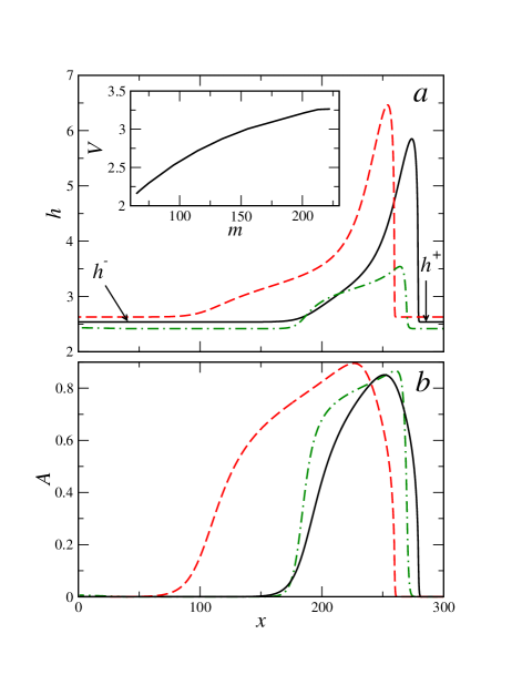
Figure 1: $h$ (a) and $A$ (b) for various values of $m$ and $\alpha$. Solid line is for $m=147.7$, $V=2.72$, dashed line is for $m=211$, $V=3.12$, for $\delta=1,\alpha=0.08,\beta=2$; point-dashed line is for $\alpha=0.025,\delta=1.15$, $m=62$, $V=0.86$. Inset: $V$ vs $m$.

In the coordinate system co-moving with the velocity $V$ Eqs. (2),(3) assume the form:

$$\frac{\partial h}{\partial t} = V\partial_{x}h-\alpha\frac{\partial h^{3}A}{\partial x}+\frac{\alpha}{\phi}\nabla\left(h^{3}A\nabla h\right)$$ (5)

$$\frac{\partial A}{\partial t} = V\partial_{x}A+\lambda_{0}A+\nabla^{2}A+\frac{8(2-\delta)}{3\pi}A^{2}-\frac{3}{4}A^{3}$$ (6)

Numerical studies revealed that the one-dimensional Eqs. (5),(6) possess a one-parametric family of localized (solitons) solutions, see Fig 1:

$$A(x,t)=A(x-Vt),h(x,t)=h(x-Vt)$$ (7)

Here the boundary conditions take a form $h\to h_{0},A\to 0$ for $x\to\pm\infty$, where $h_{0}$ is the asymptotic height. The one-dimensional steady state soliton solution (7) satisfy:

$$V(h-h_{0}) = \alpha h^{3}A\left(1-\frac{\partial_{x}h}{\phi}\right)$$ (8)

$$-V\frac{\partial A}{\partial x} = \lambda A+\partial_{x}^{2}A+\frac{8(2-\delta)}{3\pi}A^{2}-\frac{3}{4}A^{3}$$ (9)

The solutions can be parameterized by the “trapped mass” $m$ carried by the soliton, i.e. the area above $h_{0}$,

$$m=\int_{-\infty}^{\infty}(h-h_{0})dx$$ (10)

The velocity $V$ is an increasing function of $m$, see inset Fig. 1a. The structure of the solutions is sensitive to the value of $\alpha$: for large $\alpha$ the solution has a well-pronounced shock-wave shape, Fig. 1, with the height of the crest $h_{max}$ several times larger than the asymptotic depth $h_{0}$. For $\alpha\to 0$ the solution assumes more rectangular form, see Fig. 1, and $h_{max}-h_{0}\ll h_{0}$.

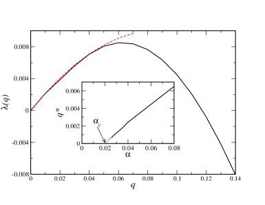
Figure 2: $\lambda(q)$ vs $q$ for $\delta=1.15$, $\alpha=0.08$ and $m=102$. Solid line: $\lambda(q)$ obtained by numerical stability analysis of one-dimensional solution Eq. (11). Dashed line is solution of Eq. (15). Inset: optimal wavenumber of $q^{*}$ vs $\alpha$ for $\delta=1.15$

To understand transverse instability we focus on the soliton solution with slowly varying position $x_{0}(y,t)$

$$A(x,t)=\bar{A}(x-x_{0}(t,y)),\;h(x,t)=\bar{h}(x-x_{0}(t,y))$$ (11)

Substituting Eq. (11) in Eq. (5) and integrating over $x$, one obtains

$$\partial_{t}m=V(m)(h^{+}-h^{-}(m))-\zeta_{1}\partial_{y}^{2}x_{0}+\zeta_{2}\partial_{y}^{2}m$$ (12)

where $\zeta_{1,2}=const$ is defined as

$$\zeta_{1}=\frac{\alpha}{\phi}\int_{-\infty}^{\infty}\left(\bar{A}\bar{h}^{3}\partial_{x}\bar{h}\right)dx,\;\zeta_{2}=\frac{\alpha}{\phi}\int_{-\infty}^{\infty}\left(\bar{A}\bar{h}^{3}\partial_{m}\bar{h}\right)dx$$

Here $h^{+}=h(x\to\infty)$ is the height of the deposit layer ahead of the front and $h^{-}=h(x\to-\infty)$ is the height behind the front, see Fig. 1a. While the value of $h^{+}$ is prescribed by the initial sediment height, the value of $h^{-}$ behind the front is determined by the velocity (or mass) of the front. For steady-state solution $h^{+}=h^{-}=h_{0}$. For the slowly-evolving solution the difference between $h^{+}$ and $h^{-}$ can be small, however it is important for the stability analysis. These terms are also necessary to describe experimentally observed initial acceleration/slowdown of the avalanches. Substituting Eqs. (11) into Eq. (3) and performing orthogonality conditions one obtains

$$\partial_{t}x_{0}=V(m)+\partial_{y}^{2}x_{0}$$ (13)

There are also higher order terms in Eq. (13) which we neglect for simplicity. To see the onset of the instability we keep only the leading terms in Eq.(12),(13), using $V(m)\approx V(m_{0})+V_{m}(m-m_{0})$, and $\tilde{m}=m-m_{0}\ll m_{0}$:

$$\partial_{t}\tilde{m} = -\tau\tilde{m}-\zeta_{1}\partial_{y}^{2}x_{0}+\zeta_{2}\partial_{y}^{2}\tilde{m}$$

$$\partial_{t}x_{0} = V_{m}\tilde{m}+\partial_{y}^{2}x_{0}$$ (14)

where $m_{0}=const$ is the steady-state mass of the soliton, and $\tau=V(m_{0})\partial_{m}h^{-}$. Seeking solution in the form $m,x_{0}\sim\exp[\lambda t+iqy]$, $q$ is the transverse modulation wavenumber, for the most unstable mode we obtain from Eq. (14) the growthrate $\lambda$

$$\lambda=\frac{-q^{2}(1+\zeta_{2})-\tau+\sqrt{(q^{2}(1-\zeta_{2})-\tau)^{2}+4V_{m}\zeta_{1}q^{2}}}{2}$$ (15)

Expanding Eq. (15) for $q\to 0$ we obtain $\lambda\approx\frac{1}{2}(2V_{m}\zeta_{1}/\tau-1)q^{2}+O(q^{4})$. The instability occurs if $V_{m}\zeta_{1}/\tau-1/2>0$. Substituting $\tau$ and using $V_{m}/h_{m}=V_{h}$, we obtain a simple instability criterion:

$$2V_{h}\zeta_{1}/V>1$$ (16)

Eq. (16) gives a value of threshold $\alpha$ since $\zeta_{1}\sim\alpha$. For $\alpha<\alpha_{c}$ no instability occurs, and the modulation wavelength diverges for $\alpha\to\alpha_{c}$. Far away from the threshold we neglect $\tau$ and then obtain for $\lambda(q)$:

$$\lambda=|q|\sqrt{\zeta_{1}V_{m}}-(1+\zeta_{2})q^{2}/2+O(q^{3})$$ (17)

The optimal wavenumber $q^{*}$ is given

$$q^{*}\sim\sqrt{\zeta_{1}V_{m}}\sim\alpha$$ (18)

Fig. 2 shows $\lambda(q)$ obtained by numerical stability analysis of linearized Eqs. (2), (3) near the one-dimensional solution Eq. (7). For comparison is shown the solution to Eq. (15), with the parameters extracted from the corresponding one-dimensional steady-state problem Eqs. (8),(9). One sees that Eq. (15) gives correct description for small $q$, however fails to predict $\lambda(q)$ in the whole range of $q$. For this purpose one needs to include higher order terms. Thus, Eq. (15) gives a correct description of the onset of instability and qualitative estimate for the selected wavenumber $q^{*}$. Inset to Fig. 2 shows the dependence of optimal wavenumber $q^{*}$ vs $\alpha$, obtained by numerical linear stability analysis of the soliton solution. It shows almost linear decrease of $q^{*}$ with $\alpha$ consistent with Eq. (18). For very small $\alpha$ the plot indicates that $q^{*}\to 0$ at $\alpha\to\alpha_{c}$, consistent with Eq. (16). From the qualitative point of view, the transverse instability of planar front is caused by the following mechanism: local increase of soliton mass results in the increase of its velocity and, consequently, the “bulging” of the front. Due to the mass conservation, the bulge depletes material in the neighboring areas and further decreases their speed.

Figure 3: Grey-coded images of $h(x,y)$ (white corresponds to larger $h$) for a) $t=170$, b) $t=300$ and c) $t=500$ units of time. Domain size is 600 units in $x$ and 450 units in $y$ direction, only part of domain in $x$ direction is shown. Parameters: $\delta=1.16$, $\alpha=0.14$, $\beta=2$ and initial height $h_{0}=2.285$.

To study the evolution of the avalanche front beyond the initial linear instability regime, a fully two-dimensional numerical analysis of Eqs. (2), (3) was performed. Integration was performed in a rectangular domain with periodic boundary conditions in $x$ and $y$ directions. The number of mesh points was up to $1200\times 600$ or higher. As an initial condition we used a flat state $h=h_{0}$ with a narrow stipe $h=h_{0}+2$ deposited along the $y$-direction. To trigger the transverse instability, small noise was added to the initial conditions. The initial conditions rapidly developed into a quasi-one-dimensional solution described by Eq. (7). Due to the periodicity in the $x$-direction, the soliton could pass through the integration domain several times. It allowed us to perform analysis in a relatively small domain in the $x$-direction. The transverse modulation of the soliton leading front was observed after about 100 units of time for the parameters of Fig. 3. We observe that modulation initially grows in amplitude, eventually coarsens and leads to the formation of large-scale finger structures.

At the qualitative level the agreement between theory and experimental results of Mallogi et al. Malloggi:2005 is impressive. (i) Existence of steady-state soliton-like avalanches propagating downhill with a shape similar to experiment. (ii) Generic zero wave number (longwave) transverse instability compatible with the experimental divergence of the selected wavelength close to the instability threshold. Far from the threshold, linear growth rate dependence with $q$ compatible with measurements. (iii) Coarsening in the later development of the instability. (iv) Fingering instability with localized droplet-like avalanches (also similar to those described in Borzsonyi:2005 ). The analysis predicts that the transverse instability ceases to exist when the rescaled transport coefficient $\alpha$ decreases (see Fig. 2). In the present form, the model does not provide an explicit relation between $\alpha$ and the chute angle $\varphi$ (since $\alpha$ depends also on $\tau_{\rho}$). Nevertheless, molecular dynamics studies indicate that the OP diffusion coefficient $D_{\rho}=l_{\rho}^{2}/\tau_{\rho}$ increases with pressure VTA03 . Since the pressure is proportional to the sediment height $h_{0}$ which increases as the angle $\varphi$ decreases, it results in the decrease of $\tau_{\rho}$. Thus, with the decrease of angle $\bar{\varphi}$ the instability should disappear, in agreement with experiment where the soliton is found stable at lower inclination angles.

An important question remains is how to bring to a more quantitative level the comparison between theory and the experimental measurements. In this perspective, a challenging question is to deeply understand the qualitative differences between smooth glass bead and rough sandy materials as far as the effective flow rules and avalanche shapes are concerned. This work calls for more systematic measurements centered on the soliton velocity dependence with the flowing mass for various materials and the possible identification of an instability threshold for glass beads. Such results would allow a more precise assessment of the model parameters and could lead the way to a reliable and predictable modelling of granular avalanches. The fingering patterns bear remarkable similarities with those existing in thin films flowing down inclined surfaces, both with clear and particle-laden fluids Troian:1989 . However, the physical mechanisms leading to this fingering are likely dissimilar: in fluid films, it is driven (and stabilized) by the surface tension, whereas in the granular flow case, the surface tension plays no role. We thank Olivier Pouliquen, Bruno Andreotti, Stephane Douady, Lev Tsimring, Tamas Börzsönyi and Robert Ecke for discussions and help. IA was supported by US DOE, Office of Science, contract W-31-109-ENG-38.

References

- (1) G.D.R. Midi, Eur. Phys. Jour. E 14, 341 (2004).
- (2) O. Pouliquen et al, Powders & Grains 2005, p. 850, ed. by R. Garcia-Rojo, H.J. Herrmann, and S. McNamaca; Balkema, Rotterdam.
- (3) A. Daerr and S. Douady, Nature (London), 399, 241 (1999) 241.
- (4) F. Malloggi, J. Lanuza, B. Andreotti, and E. Clement, Powders & Grains 2005, p. 997, ed. by R. Garcia-Rojo, H.J. Herrmann, and S. McNamaca; Balkema, Rotterdam; cond-mat/0507163, submitted to Phys. Rev. Lett. (2005)
- (5) T. Börzsönyi, T.C. Halsey, and R.E. Ecke, Phys. Rev. Lett. 94, 208001 (2005).
- (6) O. Pouliquen, J. Delour, and S.B. Savage, Nature (London) 386, 816 (1997).
- (7) I.S. Aranson and L.S. Tsimring, Phys. Rev. E64, 020301(R) (2001); Phys. Rev. E65, 061303 (2002);
- (8) I.S. Aranson and L.S. Tsimring, submitted to Rev. Mod. Phys. (2005), cond-mat/0507419
- (9) D. Volfson and L.S. Tsimring and I.S. Aranson, Phys. Rev. Lett. 90, 254301 (2003); Phys. Rev. E68, 021301 (2003); Phys. Rev. E69, 031302 (2004).
- (10) S.M. Troian, E. Herbolzheimer, S.A. Safran, and J.F. Joanny, Erophys. Lett. 10, 25 (1989); J. Zhou, B. Dupuy, A.L. Bertozzi, and A.E. Hosoi, Phys. Rev. Lett. 94, 117803 (2005).