Conduction eigenchannels of atomic-sized contacts:
$\boldsymbol{Ab\ initio}$ KKR Green’s function formalism.

Abstract

We develop a formalism for the evaluation of conduction eigenchannels of atomic-sized contacts from first-principles. The multiple scattering Korringa-Kohn-Rostoker (KKR) Green’s function method is combined with the Kubo linear response theory. Solutions of the eigenvalue problem for the transmission matrix are proven to be identical to eigenchannels introduced by Landauer and Büttiker. Applications of the method are presented by studying ballistic electron transport through Cu, Pd, Ni and Co single-atom contacts. We show in detail how the eigenchannels are classified in terms of irreducible representations of the symmetry group of the system as well as by orbital contributions when the channels wave functions are projected on the contact atom.

I Introduction

The invention of the scanning tunneling microscopeSTM in 1981 and a consequent development in the beginning of the nineties of the remarkably simple experimental technique known as mechanically controllable break junction (MCBJ)Muller ; MCBJ led to the possibility of fabrication of metallic point contacts approaching the atomic scale. The recent review article (Ref. Ruitenbeek, ) summarizes the numerous achievements in this field. In the experiments the conductance measured as a function of the elongation of the nanocontacts decreases in a stepwise fashion MCBJ ; Ohnishi ; Yanson_Nature_1 ; Cuevas_exp with steps of order of the conductance quantum $G_{0}=2e^{2}/h$. Such behavior of the conductance is attributed to atomic rearrangements that entails a discrete variation of the contact diameter. Atom_rearrang ; Brandbyge ; Todorov ; Agrait

The electron transport in metallic nanocontacts is purely ballistic and phase-coherent because their size is much smaller than all scattering lengths of the system. According to Landauer,Landauer conductance is understood as transport through nonmixing channels,

$$G=\frac{2e^{2}}{h}\sum_{n=1}^{N}T_{n},$$

where $T_{n}$’s are transmission probabilities. They are defined as eigenvalues of the transmission matrix $\mathbf{\tau\tau}^{\dagger}$. Here the matrix element $\tau_{nm}$ gives the probability amplitude for an incoming electron wave in the transverse mode (channel) $n$ on the left from the contact to be transmitted to the outgoing wave in the mode $m$ on the right. Consequently, the eigenvectors of $\mathbf{\tau\tau}^{\dagger}$ are usually called eigenchannels. It was shown in the pioneering work by Scheer et al.Scheer that a study of the current-voltage relation for the superconducting atomic-sized contacts allowed to obtain transmission probabilities $T_{n}$’s for particular atomic configurations realized in MCBJ experiments. The $T_{n}$’s are found by fitting theoretical and experimental $I-V$ curve which has a peculiar nonlinear behavior for superconducting contacts at voltages $eV$ smaller than the energy gap $2\Delta$ of a superconductorScheer . The origin of such effect is explained in terms of multiple Andreev reflections.MAR The analysis of MCBJ experiments within the tight-binding (TB) model suggested by Cuevas et al.Cuevas_TB_model ; Scheer_Nature gave a strong evidence to the relation between the number of conducting modes and the number of valence orbitals of a contact atom.

To describe the electronic and transport properties of nanocontacts, quite a big number of different methods which supplemented each other were developed during the last 15 years. Early models employed a free-electron-like approximation.Brandbyge ; FE_models ; FE_Brandbyge Further approaches based on density functional theory (DFT) used psuedopotentials to describe atomic chains suspended between jellium electrodes.Lang ; Kobayashi The TB models were applied to the problem of the conduction eigenchannelsCuevas_TB_model ; TB_models and to the study of the breaking processes of nanowires.TB_models_1 The up-to-date fully self-consistent ab initio methodsAb-initio ; Ab-initio_1 ; Rocha allowed to treat both the leads and the constriction region on the same footing and to evaluate the non-equilibrium transport properties as wellAb-initio_1 ; Rocha ; new_methods .

The scattering waves, underlying a concept of eigenchannels introduced by Landauer and Büttiker,Landauer do not form an appropriate basis for the most of ab initio methods. Instead, one considers conduction channels as eigenvectors of some hermitian transmission matrix written in terms of local, atom centered basis set.Cuevas_TB_model ; Ab-initio_1 One of the goals of the present paper is to establish a missing link between these approaches. Below we introduce a formalism for the evaluation of conduction eigenchannels, which combines an ab initio Korringa-Kohn-Rostoker (KKR) Green’s function methodSKKR for the electronic structure calculations and the Baranger and Stone formulation of the ballistic transportBarStone . In recent publications,Imp_Paper1 ; Imp_Paper2 we have successfully applied this method to the study of the electron transport through atomic contacts contaminated by impurities. In the present paper, mathematical aspects of the problem are considered, followed by some applications. In particular, we analyze the symmetry of channels and relate our approach to the orbital classification of eigenmodes introduced by Cuevas et al.Cuevas_TB_model

The paper is organized as follows. A short description of the KKR method is given in Sec. II. We proceed in Sec. III with a formal definition of eigenchannels for the case of realistic crystalline leads attached to atomic constriction. Sec. IV supplemented by Appendices A and B contains mathematical formulation of the method. Briefly, using the equivalence of the Kubo and Landauer approaches for the conductance, BarStone ; Mavropoulos we build the transmission matrix $\tau\tau^{\dagger}$ in the scattering wave representation. The angular momentum expansion of the scattering Bloch states within each cell is used further to find an equivalent, KKR representation of the transmission operator for which the eigenvalue problem can be solved. Applications of the method are presented in Sec. V. In particular, we focus on transition metal contacts (such as Ni, Co and Pd), since experimentalLudoph ; Half_int_exp ; Viret and theoretical studies PRB_MR ; TB-LMTO-Ni ; Ni_Spain ; Pt_Spain ; Ni_Smogunov of their transport properties have been attracting much attention during the last years. Experiments Huge_MR ; Huge_MR_1 ; Hua_Chopra ; Sullivan_Ni ; Chopra_Co regarding ballistic magnetoresistance (BMR) effect in ferromagnetic contacts are commented. A summary of our results is given in Sec. VI.

II Electronic structure calculation of the atomic contacts

The systems under consideration consist of two semi-infinite crystalline leads, left (L) and right (R), coupled through a cluster of atoms which models an atomic constriction. In Fig. 1 a typical configuration used in the calculations is shown — the two fcc (001) pyramids attached to the electrodes are joined via the vertex atoms. We employed the ab initio screened KKR Green’s function method to calculate the electronic structure of the systems. Since details of the approach can be found elsewhere, SKKR only a brief description is given below.

In the KKR formalism one divides the whole space into non-overlapping, space-filling cells, with the atoms (and empty spheres) positioned at the sites ${\mathbf{R}}_{n}$, so that the crystal potential $V$ is expressed in each cell as $V_{n}({\mathbf{r}})=V({\mathbf{R}}_{n}+{\mathbf{r}})$. The one-electron retarded Green’s function is expressed in terms of local functions centered at sites ${\mathbf{R}}_{n}$:

$$G^{+}({\mathbf{R}}_{n}+\ {\mathbf{r}},{\bf R}_{n^{\prime}}+\ {\mathbf{r}^{\prime}};E)$$

$$= \delta_{nn^{\prime}}\sqrt{E}\sum_{L}R_{L}^{n}({\bf r}_{<};E)H_{L}^{n}({\bf r}_{>};E)$$

$$\ +\ \sum_{LL^{\prime}}R_{L}^{n}({\bf r};E)G_{LL^{\prime}}^{nn^{\prime}}(E)R_{L^{\prime}}^{n^{\prime}}({\bf r^{\prime}};E)$$

where ${\mathbf{r}}$, ${\mathbf{r}^{\prime}}$ are restricted to the cells $n$ and $n^{\prime}$; ${\mathbf{r}}_{<}$, ${\mathbf{r}}_{>}$ denote one of the two vectors ${\mathbf{r}}$ or ${\mathbf{r}^{\prime}}$ with the smaller or the larger absolute value, and local functions $R_{L}^{n}({\bf r};E)$ and $H_{L}^{n}({\bf r};E)$ are the regular and irregular solutions of the Schrödinger equation for the single potential $V_{n}({\mathbf{r}})$. Here the index $L=(l,m)$ stands for the angular momentum quantum numbers and atomic units are used: $e=-\sqrt{2}$, $\hbar=1$, $m=1/2$. The structural Green’s function $G_{LL^{\prime}}^{nn^{\prime}}(E)$ (structure constants) in Eq. (II) is related to the known structure constants of the appropriately chosen reference system by the algebraic Dyson equation which includes the difference $\boldsymbol{\Delta t}=\delta_{nn^{\prime}}\delta_{LL^{\prime}}\Delta t^{n}_{L}$ between local $t$-matrices of the physical and a reference system. In the screened KKR methodSKKR we use a lattice of strongly repulsive, constant muffin-tin potentials (typically, $\sim 4$Ry height) as reference system that leads to structure constants which decay exponentially in real space.

Within the screened KKR method both a constriction region and the leads are treated on the same footing. This is achieved by using the hierarchy of Green’s functions connected by a Dyson equation, so that we perform the self-consistent electronic structure calculations of complicated systems in a step-like manner. First, using the concept of principal layers together with the decimation technique,2D_SKKR we calculate the structural Green’s function of the auxiliary system consisting of semi-infinite leads separated by a vacuum barrier. At the second step, the self-consistent solution of the impurity problem is found by embedding a cluster with perturbed potentials caused by the atomic contact into the auxiliary system. Due to effective screening of perturbation, the algebraic Dyson equation for the structure constants is solved in real space.SKKR

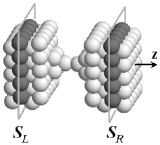
Figure 1: Geometry of an atomic constriction: two fcc (001) pyramids are attached via apex atoms. Conductance is calculated between the two planes $S_{\mathrm{L}}$ and $S_{\mathrm{R}}$ positioned in the leads.

III Definition of eigenchannels

The concept of eigenchannels is introduced in the Landauer approach to ballistic transport, where the problem of the conductance evaluation is considered from viewpoint of scattering theory. Following Landauer,Landauer we look at the system shown in Fig. 1 as consisting of two semi-infinite leads (electrodes) attached to a scattering region (atomic-sized constriction). Far away from the scattering region the propagating states are the unperturbed Bloch waves $\Psi^{\circ}_{\boldsymbol{k}}({\bf r},E)$ of the left (L, $z\to-\infty$) and right (R, $z\to+\infty$) leads, where ${\boldsymbol{k}}$ belongs to the isoenergetic surface $E=\mbox{const}$ (Fermi surface, $E=E_{F}$, in case of conductance) and a common notation $\boldsymbol{k}=(\mathbf{k},\lambda)$ is used to denote Bloch vector $\mathbf{k}$ and band index $\lambda$. For the eigenchannel problem one considers in-coming and out-going states in the L and R leads normalized to a unit flux. The in-states in L and out-states in R are ${\Phi}^{\circ}_{\boldsymbol{k}}={\Psi}^{\circ}_{\boldsymbol{k}}/\sqrt{v_{\boldsymbol{k}}}$ with positive velocity $v_{\boldsymbol{k}}\propto\mbox{v}^{z}_{\boldsymbol{k}}>0$ along $z$-axis. The conjugated states $\Phi^{\circ\,*}_{\boldsymbol{k}}=\Psi^{\circ\,*}_{\boldsymbol{k}}/\sqrt{|v_{\boldsymbol{-k}}|}$ are the out-states in L and in-states in R with negative velocity $v_{\boldsymbol{-k}}\propto\mbox{v}^{z}_{-\boldsymbol{k}}<0$. Here $\mbox{v}^{z}_{\boldsymbol{k}}$ is a $z$-component of the group velocity $\mathbf{v}_{\boldsymbol{k}}=\partial E_{\boldsymbol{k}}/\partial{\mathbf{k}}$; a proportionality factor between $v_{\boldsymbol{k}}$ and $\mathbf{v}_{\boldsymbol{k}}^{z}$ related to a particular choice of normalization of the Bloch waves is introduced further in Sec.IV.B.

The potential $\Delta V(\mathbf{r})$ describing the constriction introduces a perturbation to the perfect conductor. Let $\Phi_{\boldsymbol{k}}({\bf r},E)$ be a perturbed state which is a solution of the Lippmann-Schwinger equation for an in-coming state in L:

$$\Phi_{\boldsymbol{k}}({\bf r},E) = {\Phi}^{\circ}_{\boldsymbol{k}}({\bf r},E)$$

$$+\int d^{3}\mathbf{r^{\prime}}\ G^{+}_{0}(\mathbf{r},\mathbf{r^{\prime}},E)\Delta V(\mathbf{r^{\prime}})\Phi_{\boldsymbol{k}}(\mathbf{r^{\prime}},E)$$

where the integral goes over all space, and $G^{+}_{0}(\mathbf{r},\mathbf{r^{\prime}},E)$ is the retarded Green’s function of the perfect conductor. Asymptotic behavior of $\Phi_{\boldsymbol{k}}({\bf r},E)$ is

$$\Phi_{\boldsymbol{k}}({\bf r},E){\Bigl{.}\Bigr{|}}_{z\to-\infty} = \Phi^{\circ}_{\boldsymbol{k}}({\bf r},E)+\sum_{\boldsymbol{k^{\prime}}}\rho_{\boldsymbol{kk^{\prime}}}(E)\ {\Phi}^{\circ\,*}_{\boldsymbol{k^{\prime}}}({\bf r},E)$$

$$\Phi_{\boldsymbol{k}}({\bf r},E){\Bigl{.}\Bigr{|}}_{z\to+\infty} = \sum_{\boldsymbol{k^{\prime}}}\tau_{\boldsymbol{kk^{\prime}}}(E)\ {\Phi}^{\circ}_{\boldsymbol{\kappa^{\prime}}}({\bf r},E)$$ (3)

where $\tau_{\boldsymbol{kk^{\prime}}}(E)$ and $\rho_{\boldsymbol{kk^{\prime}}}(E)$ are transmission and reflection amplitudes, assuming elastic scattering ($E_{\boldsymbol{k}}=E=E_{\boldsymbol{k}^{\prime}}$). According to the Landauer-Büttiker formula,Landauer conductance is given by $g=g_{0}\mathrm{Tr}(\tau\tau^{\dagger})$, where trace goes over in-coming states ($\boldsymbol{k}$) in the left electrode and $E=E_{F}$. An equivalent formulation with respect to in-coming states ($-\boldsymbol{k^{\prime}}$) from the right electrode reads as $g=g_{0}\mathrm{Tr}(\tau^{\dagger}\tau)$.

Eigenchannels appear from a unitary transformation of in- and out-states. Let $\omega$ be a unitary transform of in-states in L: $\Phi^{\circ\,\mathrm{in}}_{\nu}({\bf r},E)|_{z\to-\infty}=\sum_{\boldsymbol{k}}\omega_{\nu\boldsymbol{k}}(E)\,\Phi^{\circ\,\mathrm{in}}_{\boldsymbol{k}}({\bf r},E)$. The corresponding solution $\Phi_{\nu}({\bf r})$ of Eq. (III) for an arbitrary r is

$$\Phi_{\nu}({\bf r},E)=\sum_{\boldsymbol{k}}\omega_{\nu\boldsymbol{k}}(E)\,\Phi_{\boldsymbol{k}}({\bf r},E),$$ (4)

The unitary transform $\omega$ is defined such way that the transmission matrix $T=\tau\tau^{\dagger}$ is diagonal in the basis $\nu$:

$$\omega\,(\tau\tau^{\dagger})\,\omega^{\dagger}=\mbox{diag}\{T_{\nu}\},$$ (5)

and the conductance reads as $g=g_{0}\sum_{\nu}T_{\nu}(E_{F})$, where the $T_{\nu}$’s are transmission probabilities of eigenchannels.

The matrix $\tau$, however, is not diagonal in basis $\nu$. Following Ref. Brandbyge1, one can introduce a unitary matrix $\theta$ which satisfies the equation:

$$\omega\tau\theta^{\dagger}=\theta\tau^{\dagger}\omega^{\dagger}=\mbox{diag}\{\sqrt{T_{\nu}}\},$$

where all quantities are energy dependent. The solution is $\theta=\mbox{diag}\{1/\sqrt{T_{\nu}}\}\omega\tau$. The following properties of $\theta$ can be checked: $\theta\theta^{\dagger}=\delta_{\nu\nu^{\prime}}$, $\theta^{\dagger}\theta=\delta_{\boldsymbol{kk^{\prime}}}$, thus $\theta$ is indeed the unitary matrix. It diagonalizes $\tau^{\dagger}\tau$:

$$\theta\,(\tau^{\dagger}\tau)\,\theta^{\dagger}=\mathrm{diag}\{T_{\nu}\}.$$ (6)

Matrix $\theta$ performs a unitary transform of out-states in R, so that the linear combination $\nu$ of in-coming states in L scatters into the linear combination $\nu$ of the out-states in R, $\Phi^{\circ\,\mathrm{out}}_{\nu}(\mathbf{r},E)|_{z\to+\infty}=\sum_{\boldsymbol{k}}\theta_{\nu\boldsymbol{k}}(E)\,\Phi^{\circ\,\mathrm{out}}_{\boldsymbol{k}}({\bf r},E),$ with the transmission amplitude $\sqrt{T_{\nu}(E)}$, namely: $\Phi_{\nu}(\mathbf{r},E)|_{z\to+\infty}=\sqrt{T_{\nu}(E)}\ \Phi^{\circ\,\mathrm{out}}_{\nu}(\mathbf{r},E)$.

One can showBarStone ; Mavropoulos that for the Bloch states at the same energy ($E_{\boldsymbol{k}}=E=E_{\boldsymbol{k^{\prime}}}$) in the ideal leads the following relations hold for the current matrix elements:

$$\int_{S}dS\left[\Psi^{\circ}_{\boldsymbol{k}}(\mathbf{r},E)\,i\!\stackrel{{\scriptstyle\leftrightarrow}}{{\partial_{z}}}\Psi^{\circ\,*}_{\boldsymbol{k^{\prime}}}(\mathbf{r},E)\right]\ =\ \frac{v_{\boldsymbol{k}}}{2\pi}\,\delta_{\boldsymbol{kk^{\prime}}},$$ (7)

where the Bloch waves are either left ($v_{\boldsymbol{\kappa}}\propto(\partial E_{\boldsymbol{k}}/\partial\mathbf{k})_{z}>0$) or right-travelling ($v_{\boldsymbol{\kappa}}<0$), the operator $\stackrel{{\scriptstyle\leftrightarrow}}{{\partial}}_{z}$ is defined as $f\stackrel{{\scriptstyle\leftrightarrow}}{{\partial}}_{z}g=f(\partial_{z}g)-(\partial_{z}f)g$, and the integral goes over infinite plane $S$ (cross-section of the lead) which is perpendicular to the current direction $z$.

In case of the perturbed system the orthogonality relation holds for current matrix elements in the basis of eigenchannels. Using Eqs. (3), (5) and (7) we can compute it in the asymptotic region of the right (R) lead:conjphi

$$\int\limits_{S_{R}}dS\left[\Phi_{\nu}(\mathbf{r},E)\,i\!\stackrel{{\scriptstyle\leftrightarrow}}{{\partial_{z}}}{\Phi}^{*}_{\mu}(\mathbf{r},E)\right]_{z\to+\infty}=\frac{T_{\nu}(E)}{2\pi}\,\delta_{\nu\mu}.$$ (8)

We note, that Eq. (8) holds for any position $z$ of the plane $S$. Because the wave functions of channels are solutions of the Schrödinger equation with a real potential corresponding to the same energy, the flux through arbitrary plane $S$ is conserved (a proof is similar to that of Appendix A of Ref. Mavropoulos, ).

IV Conduction eigenchannels within the KKR method

IV.1 Evaluation of conductance

To calculate the ballistic conductance, we employ the Kubo linear response theory as formulated by Baranger and Stone: BarStone

$$g = g_{0}\int_{S_{\mathrm{L}}}dS\int_{S_{\mathrm{R}}}dS\,^{\prime}$$ (9)

$$\times\ G^{+}({\bf r},{\bf r^{\prime}},E_{F})\stackrel{{\scriptstyle\leftrightarrow}}{{\partial}}_{z}\stackrel{{\scriptstyle\leftrightarrow}}{{\partial}}_{z^{\prime}}G^{-}({\bf r^{\prime}},{\bf r},E_{F}),$$

where $G^{-}$ and $G^{+}$ are retarded and advanced Green’s functions, respectively, and $g_{0}=2e^{2}/h$. The integration is performed over left ($S_{\mathrm{L}}$) and right ($S_{\mathrm{R}}$) planes which connect the leads with the scattering region (Fig. 1). The current flows in $z$ direction. The implementation of Eq. (9) within the KKR method, related convergence tests and further details were discussed in recent publication.Mavropoulos

In this paper we present a further extension of Ref. Mavropoulos, , a method for the evaluation of conduction eigenchannels. For that, we will follow closely the analysis of Refs. BarStone, ; Mavropoulos, where the equivalence of the Kubo and Landauer approaches to conductance problem was shown. We proceed in four steps: (i) we remind the KKR representation of the Bloch functions; (ii) we build up the asymptotic expansion of the Green’s function in terms of unperturbed Bloch states of the leads; (iii) we construct the transmission matrix $T=\tau\tau^{\dagger}$ in $\boldsymbol{k}$-space; (iv) finally, we find an equivalent representation of the transmission matrix within the local KKR basis. Further solution of the eigenvalue problem leads us to conduction channels. We mention here one aspect of the problem: for realistic calculations the planes $S_{\mathrm{L}}$ and $S_{\mathrm{R}}$ (see Fig. 2 for details) are usually placed in finite distance from the atomic constriction. Nevertheless, we first focus on the asymptotic limit before we discuss the realistic situation which is considered in Sec. IV.E and Appendix A.

IV.2 Atomic orbitals and Bloch functions

Let $\mathbf{r}$ be arbitrary point in the asymptotic region of the lead (Fig. 2). In the KKR method the local, energy dependent basis of atomic orbitals is defined at each unit cell $n$:

$$\phi^{n}_{L}(\mathbf{r},E) = \phi_{L}(\mathbf{r}-\mathbf{R}_{n},E)$$

$$= R_{L}(\mathbf{r}-\mathbf{R}_{n},E)\,\Theta(\mathbf{r}-\mathbf{R}_{n}),$$

where $R_{L}$’s are real regular solutions RL_functions of the Schrödinger equation for the potential $V_{n}(\mathbf{r})$ at cell $n$, and $\Theta$–function is 1 inside cell $n$ and is 0 outside it. The unperturbed Bloch function is given by expansion over atomic orbitals at all sites $n$ in the Born-von Kármán supercell:

$$\Psi^{\circ}_{\boldsymbol{k}}(\mathbf{r},E)=\sum_{nL}C_{\boldsymbol{k},nL}(E)\,\phi_{L}(\mathbf{r}-\mathbf{R}_{n},E)$$ (11)

with $C_{\boldsymbol{k},nL}(E)=e^{+i\mathbf{k}\mathbf{R}_{n}}C_{\boldsymbol{k}L}^{\,\circ}(E)$. Here the common notation $\boldsymbol{k}=(\mathbf{k},\lambda)$ for the Bloch vector $\mathbf{k}$ of the 1st Brillouin zone (BZ) and the band index $\lambda$ is used. The $C_{\boldsymbol{k}L}^{\,\circ}(E)$ are solutions of the KKR band structure equations KKR_band_str with energy $E$.

Considering a waveguide geometry, we will assume the Bloch functions to be normalized per cross section of the Born-von Kármán supercell (see Fig. 2) with open boundary conditions along $z$-axis. Thus, $C_{\boldsymbol{k},nL}(E)\propto 1/\sqrt{N_{x}N_{y}}$ with $N_{x}N_{y}$ being number of atoms per cross-section, and orthogonality condition for Bloch waves takes a form Mavropoulos :

$$\int\limits_{V}d^{3}\mathbf{r}\ \Psi^{\circ}_{\boldsymbol{k}}(\mathbf{r},E)\Psi^{\circ\,*}_{\boldsymbol{k^{\prime}}}(\mathbf{r},E^{\prime}) = \frac{V}{(N_{x}N_{y})}\delta_{\boldsymbol{k}\boldsymbol{k^{\prime}}}$$

$$= 2\pi A_{0}\,\delta(k_{z}-k^{\prime}_{z})\,\delta_{\boldsymbol{k_{\parallel}k^{\prime}_{\parallel}}}$$

$$= |{v}_{\boldsymbol{k}}|\,\delta(E-E^{\prime})\,\delta_{ss^{\prime}}\,\delta_{\boldsymbol{k_{\parallel}k^{\prime}_{\parallel}}}.$$

Here $V=L_{x}L_{y}L_{z}$ is a volume of the supercell, $A_{0}=L_{x}L_{y}/N_{x}N_{z}$ is an area of the $xy$-unit cell in the electrode, $s,s^{\prime}=\pm 1$ are signs of $k_{z}$ and $k^{\prime}_{z}$, relation $L_{z}\,\delta_{k_{z}k^{\prime}_{z}}=2\pi\,\delta(k_{z}-k^{\prime}_{z})$ has been used, and velocity $v_{\boldsymbol{k}}$ along current flow is defined as $v_{\boldsymbol{k}}=2\pi A_{0}(\partial E_{\boldsymbol{k}}/\partial\mathbf{k})_{z}$.

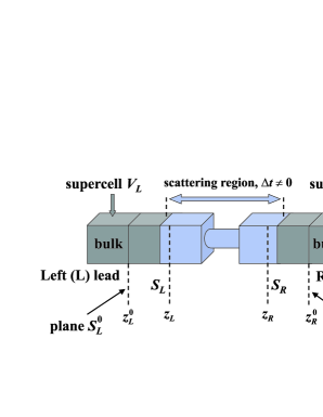
Figure 2: Sketch of the system under consideration. In a formal theory, left ($S^{0}_{\mathrm{L}}$) and right ($S^{0}_{\mathrm{R}}$) planes are placed within the leads far away from a scattering region (asymptotic limit). For all points $\mathbf{r}$ ($z<z^{0}_{\mathrm{L}}$) and $\mathbf{r^{\prime}}$ ($z^{\prime}>z^{0}_{\mathrm{R}}$) within the Born-von Kármán supercells (cubes) $V_{\mathrm{L}}$ and $V_{\mathrm{R}}$ asymptotic properties are achieved. When implementation of the method is considered, the conductance is calculated between the planes $S_{\mathrm{L}}$ and $S_{\mathrm{R}}$ positioned somewhere in the scattering region.

Since the Bloch waves form a complete set, a back transform of Eq. (11) exists:

$$\phi_{L}(\mathbf{r}-\mathbf{R}_{n},E)=\sum_{\boldsymbol{k^{\prime}}}B^{\dagger}_{nL,\boldsymbol{k^{\prime}}}(E)\,\Psi^{\circ}_{\boldsymbol{k^{\prime}}}(\mathbf{r},E_{\boldsymbol{k^{\prime}}}),$$ (12)

where $\boldsymbol{k^{\prime}}$ sum runs over all ${\mathbf{k^{\prime}}}$-points in the 1st BZ and over all bands $\lambda^{\prime}$. The $\dagger$ symbol means Hermitian conjugate. The expression for $B_{nL,\boldsymbol{k}}^{\dagger}$ can be obtained B_matrix from known matrix $C_{\boldsymbol{k},nL}$. One can prove further, that $C_{\boldsymbol{k},nL}$ and $B_{nL,\boldsymbol{k}}^{\dagger}$ obey the following orthogonality relations:

$$\sum_{nL}C_{\boldsymbol{k},nL}(E)\,B_{nL,\boldsymbol{k^{\prime}}}^{\dagger}(E) = \delta_{\boldsymbol{kk^{\prime}}},$$

$$\sum_{\boldsymbol{k}}B_{nL,\boldsymbol{k}}^{\dagger}(E)\,C_{\boldsymbol{k},n^{\prime}L^{\prime}}(E) = \delta_{nn^{\prime}}\delta_{LL^{\prime}},$$ (13)

where in the second equation a sum over $\boldsymbol{k}$ is restricted to states with $E_{\boldsymbol{k}}=E$.

IV.3 Asymptotic expansion of the Green’s function

Starting from the site angular momentum representation (II) of the retarded Green’s function within the KKR method and using Eqs. (11) and (12) we obtain the asymptotic expansion for $G^{+}(\mathbf{r},\mathbf{r^{\prime}},E)$ over the unperturbed Bloch waves: BarStone ; Mavropoulos

$$\left.G^{+}(\mathbf{r},\mathbf{r^{\prime}},E)\right|_{z,z^{\prime}\to\mp\infty}=$$

$$\qquad\qquad\sum_{\boldsymbol{kk^{\prime}}}\Psi^{\circ\,*}_{\boldsymbol{k}}(\mathbf{r},E)\,{\mathscr{A}}_{\boldsymbol{kk^{\prime}}}(E)\,\Psi^{\circ}_{\boldsymbol{k^{\prime}}}(\mathbf{r^{\prime}},E),$$

with $\mathbf{r}\in V_{\mathrm{L}}$, $\mathbf{r^{\prime}}\in V_{\mathrm{R}}$ (see Fig. 2), and

$${\mathscr{A}}_{\boldsymbol{kk^{\prime}}}(E)=$$

$$\sum_{n\in V_{\mathrm{L}}}\sum_{n^{\prime}\in V_{\mathrm{R}}}\sum_{LL^{\prime}}B_{\boldsymbol{k},nL}(E)\,G^{nn^{\prime}}_{LL^{\prime}}(E)\,B^{\dagger}_{n^{\prime}L^{\prime},\boldsymbol{k^{\prime}}}(E)$$

or in a matrix form: ${\mathscr{A}}=BGB^{\dagger}$. Formally, the $\boldsymbol{k}$-sums in Eq. (IV.3) are performed over all $\mathbf{k}$-states in the 1st BZ and over all bands $\lambda$. However, since the Green’s function for $\mathbf{r}\neq\mathbf{r^{\prime}}$ is a solution of the Schrödinger equation without a source term, only states $\boldsymbol{k,k^{\prime}}$ at the isoenergetic surface of energy $E$ contribute to the sum in the asymptotic expansion.BarStone ; Mavropoulos Therefore,

$${\mathscr{A}}_{\boldsymbol{kk^{\prime}}}(E)=\frac{1}{N_{z}^{2}}\ \overline{\delta}(E-E_{\boldsymbol{k}})\,\overline{\delta}(E-E_{\boldsymbol{k^{\prime}}})A_{\boldsymbol{kk^{\prime}}}(E),$$ (16)

where $\overline{\delta}(E-E_{\boldsymbol{k}})=\left({\Omega_{0}}/{S_{\lambda}}\right)\,|\mathbf{v}_{\boldsymbol{k}}|\,\delta(E-E_{\boldsymbol{k}})$. Here $N_{z}$ is number of atom sites in Born-von Kármán supercell along $z$ axis, $\Omega_{0}=(2\pi)^{3}/V_{0}$ is volume of the 1st BZ, $S_{\lambda}$ is the area of the isoenergetic surface corresponding to band $\lambda$, $\mathbf{v}_{\boldsymbol{k}}=\partial E_{\boldsymbol{k}}/\partial{\mathbf{k}}$. For the discrete $\boldsymbol{k}$-points, the function $(1/N_{z})\overline{\delta}(E-E_{\boldsymbol{k}})$ equals 1 if $E=E_{\boldsymbol{k}}$, and is 0 otherwise. In addition, boundary conditions for the Green’s functionBarStone constrain matrix elements $A_{\boldsymbol{kk^{\prime}}}(E)$ to be non-zeros only if $\boldsymbol{k}$ and $\boldsymbol{k^{\prime}}$-states are right-travelling waves (with positive velocity along $z$-axis) that corresponds to the in-states $\boldsymbol{k}$ in the left lead and out-states $\boldsymbol{k^{\prime}}$ in the right one.

IV.4 Transmission matrix: asymptotic limit

We proceed further, and use the asymptotic representation (IV.3) of the Green’s function to evaluate conductance according to Eq. (9). Assuming the integration planes to be placed within the leads infinitely far from the scattering region, we obtain:

$$g=g_{0}\mathrm{Tr}_{(\boldsymbol{k})}\left[V_{\mathrm{L}}\,{\mathscr{A}}(E_{F})\,V_{\mathrm{R}}\,{\mathscr{A}^{\dagger}}(E_{F})\right],$$ (17)

where the diagonal operators of velocities $V_{\mathrm{L}}$ and $V_{\mathrm{R}}$ (related to the left and right planes) acting in the $\boldsymbol{k}$-space were introduced: $\bigl{[}V_{\mathrm{L(R)}}\bigr{]}_{\boldsymbol{kk^{\prime}}}=\left({v_{\boldsymbol{k}}}/{2\pi}\right)\delta_{\boldsymbol{kk^{\prime}}}$. Formally, the trace (Tr) in Eq. (17) goes over all $\boldsymbol{k}$-states and the Fermi surface is taken into account by means of Eq. (16) where $E=E_{F}$.

The velocity operators can be decomposed into sum of two operators related to the Bloch states with positive and negative velocities along $z$: $\hat{V}=\hat{V}^{+}+\hat{V}^{-},$ where $\hat{V}^{+}$ is nonzero for right-travelling waves only, while $\hat{V}^{-}$ is nonzero for left-travelling ones. In the asymptotic limit, only in-coming and out-going $\boldsymbol{k}$-states with positive velocities contribute to the sums in Eq.(17). Using the relation between expansion coefficients $A_{\boldsymbol{kk^{\prime}}}$ and the transmission amplitudes $\tau_{\boldsymbol{kk^{\prime}}}$ derived in Refs. BarStone, ; Mavropoulos, ,

$$A_{\boldsymbol{kk^{\prime}}}(E)\ =\ -2\pi i\,\frac{\tau_{\boldsymbol{kk^{\prime}}}(E)}{\sqrt{v_{\boldsymbol{k}}v_{\boldsymbol{k^{\prime}}}}},$$ (18)

we obtain:

$$g = g_{0}\mathrm{Tr\,}_{(\boldsymbol{k})}\left[V^{+}_{\mathrm{L}}\,{\mathscr{A}}(E_{F})\,V^{+}_{\mathrm{R}}\,{\mathscr{A}}^{\dagger}(E_{F})\right]$$

$$= g_{0}\mathrm{Tr}_{(\boldsymbol{k})}\,[T(E_{F})],$$

where a representation of $T=\tau\tau^{\dagger}$ in $\boldsymbol{k}$-space is given by

$$T(E)=(V^{+}_{\mathrm{L}})^{1/2}\,{\mathscr{A}}(E)\,V^{+}_{\mathrm{R}}\,{\mathscr{A}}^{\dagger}(E)\,(V^{+}_{\mathrm{L}})^{1/2}$$ (20)

with a positive definite operator under square-roots.

The $\boldsymbol{k}$-representation is formal but not suitable for implementation. To solve the eigenvalue problem for $T=\tau\tau^{\dagger}$ the mapping on the site-angular momentum $(n,L)$-space of the KKR method should be presented. Such mapping is realized through the expansion (11) of the Bloch functions over atomic orbitals, so that velocity operators in $\boldsymbol{k}$-space take a form:

$$\bigl{[}V_{\mathrm{L(R)}}\bigr{]}_{\boldsymbol{kk^{\prime}}}=\sum_{nn^{\prime}\in S^{0}_{\mathrm{L}}}\sum_{LL^{\prime}}C_{\boldsymbol{k},nL}\,\bigl{[}D_{\mathrm{L(R)}}\bigr{]}^{nn^{\prime}}_{LL^{\prime}}\,C^{\dagger}_{n^{\prime}L^{\prime},\boldsymbol{k^{\prime}}},$$

where site-diagonal operators $D_{\mathrm{R}}$ and $D_{\mathrm{L}}$ defined on atomic orbitals are the KKR-analogue of velocities: KKR_velocity

$$\bigl{[}D_{\mathrm{L(R)}}(E)\bigr{]}^{nn^{\prime}}_{LL^{\prime}}\ =$$

$$\pm\,\delta_{nn^{\prime}}\,\int_{S^{n}_{\mathrm{L(R)}}}dS\left[R^{n}_{L}({\bf r},E)\,i\stackrel{{\scriptstyle\leftrightarrow}}{{\partial_{z}}}R^{n}_{L^{\prime}}({\bf r},E)\right]$$

here integral is restricted to the cross-section of the unit cell around site $n$. Now we can evaluate conductance according to Eq.(17). Taking into account that $B^{\dagger}C=C^{\dagger}B=\delta_{nn^{\prime}}\delta_{LL^{\prime}}$ [Eq.(13)], we obtain:

$$g=g_{0}\mathrm{Tr}_{(n,L)}\left(D_{\mathrm{L}}\,G\,D_{\mathrm{R}}\,G^{\dagger}\right),$$ (22)

here (and further) all matrices are assumed to be taken at the Fermi energy, $G=\{G_{LL^{\prime}}^{nn^{\prime}}\}$ stands for matrix notation of the structural Green’s function introduced in Eq. (II), and trace (Tr) involves sites and orbitals related to the atomic plane $S^{0}_{\mathrm{L}}$ (Fig. 2).

The operators $D_{\mathrm{L}}$, $D_{\mathrm{R}}$ are anti-symmetric and hermitian, thus their spectrum consists of pairs of positive and negative eigenvalues: $\pm\delta^{0}_{i}$. Let $U$ be the unitary transform of matrix $D$ (either $D_{\mathrm{L}}$ or $D_{\mathrm{R}}$) to a diagonal form:

$$D^{0}=U^{\dagger}DU=\mathrm{diag}\{\pm\delta^{0}_{i}\}.$$ (23)

Decomposition of operator ${D}$ into two terms, $D=D^{+}+D^{-}$, related to the right- and left-travelling waves is naturally given in the basis of eigenvectors:

$$D^{\pm}=UD^{0(\pm)}U^{\dagger}$$ (24)

with

$$D^{0(+)}\ =\ \left(\begin{array}[]{cc}\Delta^{+}&0\\ 0&0\end{array}\right),\qquad D^{0(-)}\ =\ \left(\begin{array}[]{cc}0&0\\ 0&-\Delta^{-}\end{array}\right),$$

where $\Delta^{+}$, $\Delta^{-}$ are positive (non-negative) diagonal matrices. The analogue of Eq. (IV.4) reads as

$$g|_{z,z^{\prime}\to\mp\infty}=g_{0}\mathrm{Tr}_{(n,L)}\left(D^{+}_{\mathrm{L}}\,G\,D^{+}_{\mathrm{R}}\,G^{\dagger}\right).$$ (25)

Now we are ready to build the $(n,L)$-representation for transmission matrix $T=\tau\tau^{\dagger}$. For that, one should extract a square-root from the positive definite operator $V^{+}_{\mathrm{L}}=CD^{+}_{\mathrm{L}}C^{\dagger}$ defined on $\boldsymbol{k}$-space with help of $(n,L)$-space. Namely, because the $V^{+}_{L}$ is positive definite, it can be represented in the following form: Gantmacher $V^{+}_{\mathrm{L}}=\Omega_{\mathrm{L}}\Omega^{\dagger}_{\mathrm{L}}$. Here an operator $\Omega_{\mathrm{L}}$ maps the $\boldsymbol{k}$-space on the $(n,L)$-space, $\Omega_{\mathrm{L}}:\{\boldsymbol{k}\}\to\{n,L\}$. The solution for $\Omega_{L}$ is

$$\Omega_{\mathrm{L}}=C(D^{+}_{\mathrm{L}})^{1/2}\,\cal{E},$$

where $\cal{E}$ is an arbitrary unitary matrix (${\cal{E}\cal{E}^{\dagger}}=1$) and $(D^{+}_{\mathrm{L}})^{1/2}=U_{L}[D^{0(+)}_{\mathrm{L}}]^{1/2}U^{\dagger}_{L}$ with $[D^{0(+)}_{\mathrm{L}}]^{1/2}$ being square-root of the positive definite diagonal matrix [Eq.(24)].

To find $T=\tau\tau^{\dagger}$, we start from Eq. (IV.4) and proceed as follows:

$$g = g_{0}\mathrm{Tr\,}_{(n,L)}\left(\Omega_{\mathrm{L}}\Omega^{\dagger}_{\mathrm{L}}\,{\cal{A}}\,V^{+}_{\mathrm{R}}{\cal{A}}^{\dagger}\right)$$

$$= g_{0}\mathrm{Tr\,}_{(n,L)}\left(\Omega^{\dagger}_{\mathrm{L}}\,{\cal{A}}\,V^{+}_{\mathrm{R}}{\cal{A}}^{\dagger}\Omega_{\mathrm{L}}\right)$$

$$= g_{0}\mathrm{Tr\,}_{(n,L)}\left[(D^{+}_{\mathrm{L}})^{1/2}C^{\dagger}\bigl{(}BG{B}^{\,\dagger}\bigr{)}\bigl{(}{C}D^{+}_{\mathrm{R}}{C}^{\dagger}\bigr{)}\right.$$

$$\left.\times\bigl{(}{B}G^{\,\dagger}B^{\dagger}\bigr{)}C(D^{+}_{\mathrm{L}})^{1/2}\,\right]$$

where Eq.(IV.3) was used. Because of $B^{\dagger}C=\delta_{nn^{\prime}}\delta_{LL^{\prime}}$ [Eq. (13)], we obtain:

$$g=g_{0}\mathrm{Tr\,}_{(n,L)}({\cal{T}}),$$ (26)

where, in the asymptotic limit, the transmission matrix $T=\tau\tau^{\dagger}$ in $(n,L)$-representation is given by

$${\cal{T}}=(D^{+}_{\mathrm{L}})^{1/2}G\,D^{+}_{\mathrm{R}}\,G^{\,\dagger}(D^{+}_{\mathrm{L}})^{1/2}.$$ (27)

The trace in Eq.(26) goes over all sites $n$ and orbitals $L$ of the atomic plane $S^{0}_{\mathrm{L}}$ in the left lead (Fig. 2). Equivalent formula can be written for the right lead. To conclude, one can prove that spectrum of the obtained matrix coincides with spectrum of transmission matrix $T$ [Eq. (20)] defined in $\boldsymbol{k}$-space (see Appendix B for details). Therefore, solution of the eigenvalue problem for $\cal{T}$ gives us required transmission probabilities.

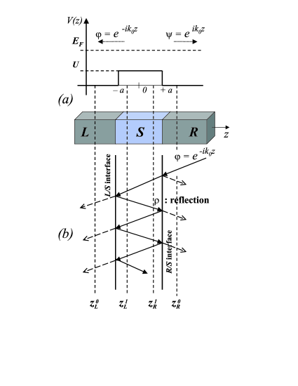
Figure 3: Top (a): A model step-like potential for the free-electron gas within the $L/S/R$ structure having two dimensional periodicity. The electrons moving with energy $E=E_{F}$ from the leads (L and R) are scattered at the potential step $U$. The $\boldsymbol{k_{\parallel}}$ momentum is conserved, while the momentum $k_{z}$ along $z$-axis is $k_{0}=\left[2mE-\boldsymbol{k}_{\parallel}^{2}\right]^{1/2}$ in the leads, and $k_{1}=\left[2m(E-U)-\boldsymbol{k}_{\parallel}^{2}\right]^{1/2}$ in the S layer. Bottom (b): A multiple reflection of the in-coming from the R lead wave $e^{-ik_{0}z}$ within the spacing layer $S$, where it is a linear combination $\phi(z)=\chi_{+}(z)+\chi_{-}(z)=\alpha\,e^{-ik_{1}z}+\beta\,e^{+ik_{1}z}$ of two functions. If $z_{L}^{1}$ is position of one of the planes taken for the conductance evaluation, transmission $T(\boldsymbol{k}_{\parallel})$ of channel $\boldsymbol{k}_{\parallel}$ is proportional to the current $j=\phi(z)\ i\!\stackrel{{\scriptstyle\leftrightarrow}}{{\partial_{z}}}\phi^{*}(z)=2k_{0}=2k_{1}|\alpha|^{2}-2k_{1}|\beta|^{2}=j_{+}-j_{-}$, which is sum of two terms (positive and negative) due to contributions from two functions, $\chi_{+}(z)$ and $\chi_{-}(z)$. The value $\rho=\beta/\alpha=(k_{1}-k_{0})/(k_{1}+k_{0})e^{+2ik_{1}a}$ has a meaning of the reflection coefficient of the S/R or S/L interface. However, if plane is chosen in the asymptotic region of the lead, at point $z_{\mathrm{L}}^{0}$, transmission $T(\boldsymbol{k}_{\parallel})\sim 2k_{0}$ contains only one positive contribution.

IV.5 General case: arbitrary positions of planes

In practical calculations of conductance with the use of the Kubo formula, the left (L) and right (R) planes are positioned somewhere in the leads (Fig. 2). Expression (22) is valid in general case and result is exactly the same as in Ref. Mavropoulos, . Operator $D_{\mathrm{L}}$ in Eq.(22) is sum of two terms: $D_{\mathrm{L}}=D^{+}_{\mathrm{L}}+D^{-}_{\mathrm{L}}$. Therefore, we can write down

$$g = g_{0}\mathrm{Tr}\left(D^{+}_{\mathrm{L}}\,G\,D_{\mathrm{R}}\,G^{\dagger}\right)+g_{0}\mathrm{Tr}\left(D^{-}_{\mathrm{L}}\,G\,D_{\mathrm{R}}\,G^{\dagger}\right)$$ (28)

$$= g^{+}+g^{-},$$

where $g^{+}$ and $g^{-}$ denote two contributions. In a formal theory, when the atomic plane $S_{\mathrm{L}}$ is placed in the asymptotic region of the left lead far from the atomic constriction the second term $g^{-}$ in Eq.(28) is equal to zero. In practice, the real space summation of current contributions includes only a finite number of sites at both atomic planes, because the current flow along $z$ direction is localized in the vicinity of the contact. Due to numerical effort we are forced to take integration planes closer to the constriction in order to obtain convergent value for the conductance with respect to number of atoms included in summation. In addition, even better convergence for matrix elements is required to solve the eigenvalue problem. A compromise can be usually achieved but positions of the atomic planes $S_{\mathrm{L}}$ and $S_{\mathrm{R}}$ do not meet the asymptotic limit criterion. However, since the electron current through the structure is conserved, any position of the planes is suitable for the calculation of conductance. If $S_{\mathrm{L}}$ is placed somewhere in the scattering region we have to sum up all multiple scattering contributions. We show in Appendix A, that all multiple scattering contributions in direction of the current cause $g^{+}$, whereas all scattering contributions in opposite direction give rise to $g^{-}$. Thus, the first term, $g^{+}$, in Eq. (28) is always positive, while the second one, $g^{-}$, is always negative. To make this statement clear, an illustration of scattering events is shown in Fig. 3 assuming a simple free-electron model. In the region of the lead where the potential is a small perturbation with respect to the bulk potential the contribution to the conductance due to $g^{-}$ is one order of magnitude smaller than $g^{+}$.

To find transmission probabilities of eigenchannels, one has to apply the procedure introduced in the previous section independently for both terms, $g^{+}$ and $g^{-}$. We refer to Appendix A for a mathematical justification. Expression for conductance takes a form:

$$g=g_{0}\mathrm{Tr\,}_{(n,L)}({\cal{T}}^{+})+g_{0}\mathrm{Tr\,}_{(n,L)}({\cal{T}}^{-}),$$ (29)

with

$${\cal{T}}^{\pm}=\pm{(\pm D^{\pm}_{\mathrm{L}})}^{1/2}\,G\,D_{\mathrm{R}}\,G^{\,\dagger}{(\pm D^{\pm}_{\mathrm{L}})}^{1/2}.$$ (30)

We show in Appendix A that all eigenvalues of ${\cal T}^{+}$ are either positive or zeros whereas all eigenvalues of ${\cal T}^{-}$ are negative or zeros. To identify transmission probabilities $T_{n}$ of channels the spectra of operators ${\cal T}^{+}$ and ${\cal T}^{-}$ have to be arranged in a proper way. Then transmission of the $n$-th channel is given by $T_{n}=\tau^{+}_{n}-\tau^{-}_{n}$, where $\pm\tau_{n}^{\pm}$ are positive and negative eigenvalues of the operators ${\cal T}^{+}$ and ${\cal T}^{-}$, respectively. The $T_{n}$ does not depend on the positions of the left ($S_{\mathrm{L}}$) and right ($S_{\mathrm{R}}$) planes, while $\tau^{\pm}_{n}$ are $z$-dependent. In the asymptotic limit $\tau^{-}_{n}|_{z_{L}\to-\infty}\to 0$ and $T_{n}=\tau^{+}_{n}|_{z_{L}\to-\infty}$, so that the Landauer picture is restored.

In general case the direct way to find the pairs of eigenvalues is not evident without a back transform to the $\boldsymbol{k}$-space. However, from the point of view of applications to the extremely small symmetric atomic contacts, as the ones we are studying in this work, the problem is easy to handle. Since the number of contributing eigenmodes is limited, the pairs of eigenvalues can be found by symmetry analysis of the eigenvectors of ${\cal T}^{+}$ and ${\cal T}^{-}$. Namely, using the symmetry properties of the structural Green’s function $G^{nn^{\prime}}_{LL^{\prime}}$ and current matrix elements $D^{nn^{\prime}}_{LL^{\prime}}$ one can show that channel’s transmission $T_{n}$ bounded between 0 and 1 is defined by eigenvalues $\tau_{n}^{+}$ and $\tau_{n}^{-}$ which belong to the same irreducible representation of the symmetry point group.

V Applications of the method

In recent papers Imp_Paper1 ; Imp_Paper2 we have verified the method described here by studying systematic changes in the conductance of metallic constrictions in the presence of defect atoms. Illustrative examples presented below focus on single-atom contacts made of pure metals such as Cu, Ni, Co and Pd.

Copper serves mainly for test purposes. It is a representative of the noble metals and has electronic properties similar to Ag and Au, for which a lot of experimental results Brandbyge ; Krans ; Exp_noble_metals ; Ludoph ; Enomoto ; Yanson_PhD as well as DFT based calculations TB_models ; Ab-initio_1 are available. In particular, a large number of experiments for alkali metals (Li, Na, K) Ludoph ; Yanson_PhD ; Yanson_Nature and noble metals (Au, Ag, Cu), Brandbyge ; Exp_noble_metals ; Ludoph ; Enomoto ; Yanson_PhD employing different techniques under room an liquid-He temperatures, show that conductance histograms have a dominant peak very close to one conductance quantum $G_{0}=2e^{2}/h$, and smaller peaks close to integer values.

However, for transition metal contacts (examples of which are Ni, Co and Pd) the situation differs significantly.Ludoph ; Enomoto Only one broad maximum centered somewhere between $1\,G_{0}$ and $3\,G_{0}$ is usually observed in conductance histograms.Ruitenbeek ; Yanson_PhD That is a signature of the nontrivial decomposition of conductance consisting of more than one perfectly transmitting channel, Cuevas_TB_model ; Scheer_Nature since for transition metal atoms $d$ states of different symmetry are available at the Fermi level. The question on half-integer conductance quantization has been addressed.Half_int_FM ; Half_int_exp However, recent experiments Untiedt do not confirm this hypothesis thus pointing to the conclusion that the electron transport through ferromagnetic contacts can never be fully spin-polarized. Another issue is a large magnetoresistance (MR) effect Huge_MR ; Huge_MR_1 ; Hua_Chopra observed for metallic point contacts made of different magnetic materials. This field is known to be full of controversy. There is still a continuing discussion on whether or not the enormous MR values found experimentally could be of electronic origin Electr_origin ; Tagirov ; Velev_Butler ; PRB_MR ; NiO_surface ; Ni_Spain ; NiO_Spain or the effect is just due to atomic rearrangements in the neck region of a contact as a response to the applied magnetic field.Magnetostriction1 ; Magnetostriction2 Extensive discussion on this topic can be found in the recent review paper by Marrows. Marrows We will comment further on the above issues.

V.1 Computational details

An atomic configuration of a constriction used in our calculations is presented in Fig. 1. The single atom contact was modeled by a small cluster attached to the semi-infinite fcc (001) leads. The cluster consists of two pyramids joined via the vertex atoms separated by a distance $a_{0}/\sqrt{2}$ . Here $a_{0}$ is the experimental lattice constant of fcc metals: 6.83 a.u. for Cu, 6.66 a.u. for Ni, 6.70 a.u. for Co, and 7.35 a.u. for Pd. The metals under consideration do not have a tendency to form chains.Chains An atomic bridge is most likely to be broken just after the single atom limit is achieved. Thus, a configuration shown in Fig. 1 resembles one of limiting configurations of point contacts which could appear in the MCBJ experiments.

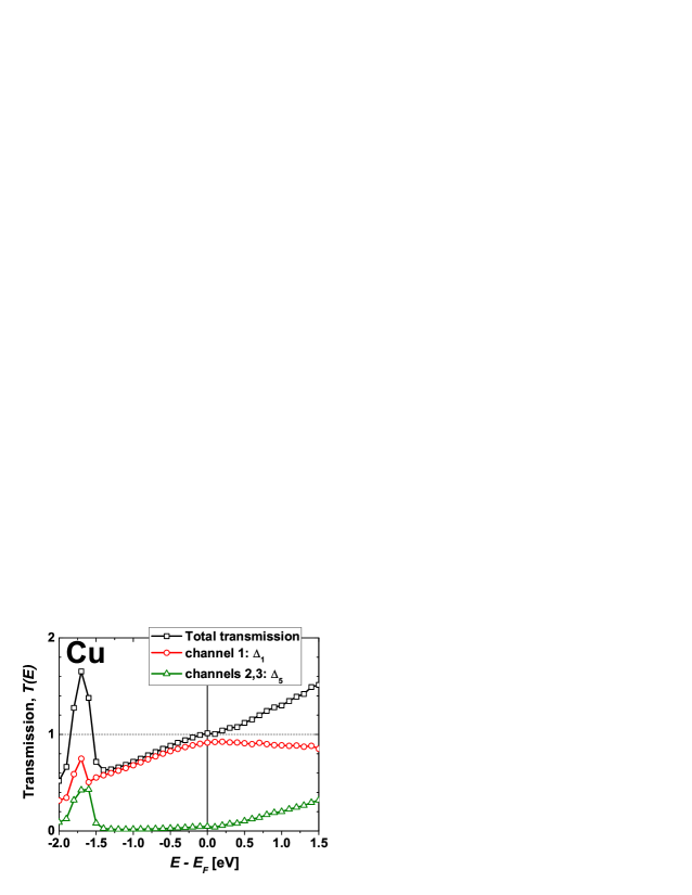
Figure 4: (Color online) Energy-dependent transmission and its decomposition to the conduction eigenchannels for the Cu single atom contact shown in Fig. 1.

Our calculations are based on DFT within the local density approximation. The parametrization of Vosko, Wilk, and Nusair Vosko_Wilk_Nusair for the exchange and correlation energy was used. The potentials were assumed to be spherically symmetric around each atom (atomic sphere approximation, ASA). However, the full charge density, rather than its spherically symmetric part, was taken into account. To achieve well converged results the angular momentum cut-off for the wave functions and the Green’s function was chosen to be $l_{\rm{max}}=3$ that imposed a natural cut-off $2l_{\rm{max}}=6$ for the charge density expansion. In case of heavy element Pd the scalar relativistic approximationSRA was employed. For the conductance calculation the surface Green’s function was computed using a small imaginary part ${\rm Im}E=0.04\,{\rm mRy}$ and about 250.000 k-points were taken in the 2D Brillouin zone. Instead of integration over planes, current matrix elements (IV.4) were averaged over atomic layers as described in detail in Ref. Mavropoulos, . A typical error in the calculation of conductance was $\sim 5\%$.

V.2 Symmetry analysis of eigenchannels

To understand the relation between the electronic structure and the transport properties of atomic contacts we consider the energy-dependent total transmission, $T(E)$, and its decomposition to the conduction eigenchannels, $T_{i}(E)$. Results are shown in Figs. 4, 6, 8, 9 for the case of Cu, Ni, Co and Pd point contacts, respectively. The investigated structure (Fig. 1) has a $C_{4v}$ symmetry. Further we denote individual channels by the indices of irreducible representations of this group using notations of Ref. Wigner, , common in band theory. In addition, each channel can be classified according to the angular momentum contributions when the channel wave function is projected on the contact atom of the constriction. This is very helpful since the channel transmission can be related to the states of the contact atom.Cuevas_TB_model For example, the identity representation $\Delta_{1}$ of the $C_{4v}$ group is compatible with the $s$, $p_{z}$ and $d_{z^{2}}$ orbitals (here the $z$ is perpendicular to the surface and passes through the contact atom), while the two-dimensional representation $\Delta_{5}$ is compatible with the $p_{x}$, $p_{y}$, $d_{xz}$, $d_{yz}$ orbitals. The basis functions of $\Delta_{2}$ and $\Delta_{2^{\prime}}$ are $d_{x^{2}-y^{2}}$ and $d_{xy}$ harmonics, respectively.

V.3 Cu contacts

The energy-dependent transmission of Cu atomic contact (shown in Fig. 1) is presented in Fig.4 together with the eigenchannel decomposition. At the Fermi energy the calculated conductance value is $G=1.01\ G_{0}$. It mainly consists of one open channel of $\Delta_{1}$ symmetry which arises locally from $s$, $p_{z}$ and $d_{z^{2}}$ orbitals when the wave function is projected on the contact atom. This result is in a good agreement with a lot of experimentsLudoph ; Yanson_PhD mentioned previously as well as with other calculations involving different approaches.TB_models ; Ab-initio_1 The additional twofold degenerate channel has $\Delta_{5}$ symmetry. Transmission of this channel increases at energies above the Fermi level ($E_{F}$) together with an increase of the $p_{x},p_{y}$ contribution to the local density of states (LDOS) at the contact atom. However, at $E<-1.5$ eV below the $E_{F}$ the $\Delta_{5}$ channel is built mainly from the $d_{xz},d_{yz}$ orbitals of the Cu atom.

We would like to point out that in case of noble metals the conductance of single-atom contact is not necessarily restricted to one channel. An example of a configuration which has more channels (but still has only one Cu atom at the central position) is presented on the top of Fig. 5. Because of the larger opening angle for incoming waves as compared with the preceding case, conductance of such system is $G=2.57\,G_{0}$ with major contribution from four channels (Fig. 5 and its caption). The value $2.57\,G_{0}$ correlates with a position of the third peak in the conductance histogram of Cu, which is shifted from $3\,G_{0}$ to smaller values.Yanson_PhD ; Ludoph As it is seen from the presented example, conductance quantization does not occur for the metallic atomic-sized contacts. In general, even for noble metals, conduction channels are only partially openLudoph in contrary to the case of quantum point contacts realized in the two-dimensional electron gas where a clear conductance quantization was observed.2DEG

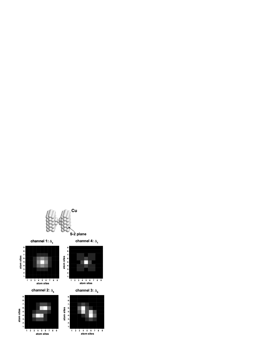
Figure 5: Wave functions $|\Psi_{i}(\mathbf{r})|^{2}$ (probability densities) of the four dominating eigenchannels for the pyramidal Cu contact shown on the top. Wave functions resolved to atoms are visualized 2 atomic planes below the surface plane (S-2). Colors from white to black correspond to consequently decreasing positive values. Transmission probabilities of channels are: $T_{1}=0.90\ (\Delta_{1})$, $T_{2}=T_{3}=0.71\ (\Delta_{5})$, $T_{4}=0.08\ (\Delta_{1})$, which are summed up to conductance $G=2.57G_{0}$. Further details are given in the text.

For illustration, we present in Fig. 5 probability amplitudes of the eigenchannles $|\Psi_{i}(\mathbf{r})|^{2}$ in real space resolved with respect to atoms of the 2nd plane (S-2) below the surface. We see that the wave functions of the 1st and the 4th channel with the highest symmetry ($\Delta_{1}$) obey all eight symmetry transformations of the $C_{4v}$ group, while two different wave functions of the double degenerate channel ($\Delta_{5}$) are transformed to each other after some symmetry operations.

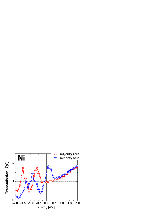
Figure 6: (Color online) Spin-dependent transmission as a function of energy for the Ni single atom contact shown in Fig. 1.

V.4 Transition metal contacts

We turn to transition metals, and consider the ferromagnetic Ni assuming a uniform magnetization of the sample. Transmission $T(E)$ split per spin of a Ni contact is shown in Fig. 6. A shift about $\sim 0.8$ eV along the energy axis between transmission curves is seen that is in agreement with exchange-splitting of the Ni $d$ states. Similar computational results regarding transmission of Ni constrictions were reported by Solanki et al.,TB-LMTO-Ni Rocha et al.Rocha  and Smogunov et al..Ni_Smogunov Exchange splitting estimated from their works varies from 0.8 eV till 1.0 eV, but fine details differ because of different atomic configurations and employed methodologies. In this regard, exchange splitting about 2.0 eV observed in transport calculations of Jacob et al.Ni_Spain  in case of Ni contact seems to be overestimated.

The shift in energy due to different spins is observed as well for the transmissions of individual channels (Fig. 7). We see from Fig. 7 and Table I that at the Fermi energy the spin-up (majority) conductance of Ni contact is mainly determined by one open $\Delta_{1}$ channel (similar to the case of Cu), while three partially open channels, of $\Delta_{1}$ and $\Delta_{5}$ symmetry, contribute to the spin-down (minority) conductance. The minority $\Delta_{5}$ channel arises locally from $d_{xz}$ and $d_{yz}$ states, rather than from $p_{x},p_{y}$ states whose contribution to the spin-down LDOS at the Fermi energy is much smaller (Fig. 7). The calculated conductance, $G=1.20\,G_{0}$, correlates with a position of the wide peak in the conductance histogram of Ni centered between $1\,G_{0}$ and $2\,G_{0}$.Yanson_PhD ; Untiedt

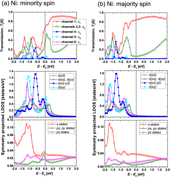
Figure 7: (Color online) Spin- and energy-dependent transmission decomposed to conduction eigenchannels for the Ni atomic-sized constriction in comparison with the symmetry projected local density of states at the contact atom (i.e. apex atoms in Fig. 1).

Table 1: Transmission probabilities of eigenchannels at the Fermi energy of Ni and Co atomic contacts shown in Fig. 1 for two different (P and AP) orientations of magnetizations in the leads. Only transmissions of the dominant channels are presented. Magnetoresistance ratio defined as $\mathrm{MR}=(G_{P}-G_{AP})/G_{AP}\times 100\%$ is given in the last line.

	Ni			Co
Channel	P		AP	P		AP
	($\downarrow$)–spin	($\uparrow$)–spin	($\uparrow$) or ($\downarrow$) spin	($\downarrow$)–spin	($\uparrow$)–spin	($\uparrow$) or ($\downarrow$) spin
$T_{1}\ (\Delta_{1})$	0.68	0.84	0.82	0.36	0.89	0.58
$T_{2}=T_{3}\ (\Delta_{5})$	0.35	0.06	0.31	0.14	0.07	0.09
$T_{4}\ (\Delta_{2})$				0.17
Transmission	1.44	0.96	1.45	0.83	1.03	0.76
MR ratio		$-17\%$			$+23\%$

Within the energy range shown in Figs. 6 and 7 ($\pm 2$ eV around $E_{F}$), we count six eigenmodes of different symmetry for both spins. At energies well above the Fermi level ($E>1.0$ eV) the spin-splitting of $sp$ Ni states is lost, and the picture is similar to what we have seen for Cu. Three channels are present: one open $\Delta_{1}$ ($sp_{z}$-like) channel with transmission around 0.9 and a partially open double degenerate $\Delta_{5}$ ($p_{x},p_{y})$ channel whose transmission increases monotonically as a function of energy. However, below the Fermi energy all eigenmodes $T_{i}(E)$ display a complicated behavior (Fig. 7, upper plots) that reflects a complex structure of the LDOS projected on orbitals of the contact atom (Fig. 7, bottom plots). Below $E_{F}$ the existing $s$, $p_{z}$ and $d_{z^{2}}$ states are strongly hybridized giving rise to two channels of $\Delta_{1}$ symmetry at energies about $E\approx-1.0$ eV and $E\approx-1.5$ eV for minority and majority spins, respectively. A clear correlation between the symmetry projected LDOS and $T_{i}(E)$ is seen for the pure $d$-channels, $\Delta_{2}$ ($d_{x^{2}-y^{2}}$) and $\Delta_{2^{\prime}}$ ($d_{xy}$). For example, the minority spin $d_{x^{2}-y^{2}}$ resonance centered around $E=-0.7$ eV and majority spin $d_{x^{2}-y^{2}}$ resonance at $E=-1.3$ eV reflect themselves as peaks in the transmission of the minority and majority $\Delta_{2}$ channels. The same is valid for the $d_{xy}$ states at $E=-1.1$ eV (spin down) and $E=-1.7$ eV (spin up) which cause the increase of transmission of the $\Delta_{2^{\prime}}$ channel at the same energies. However, even at the resonances, the $\Delta_{2}$ and $\Delta_{2^{\prime}}$ channels are only partially open because the $d_{x^{2}-y^{2}}$ and $d_{xy}$ orbitals are spread perpendicular to wire ($z$-) axis that prevents effective coupling with the neighboring atoms.

Our results for Co constriction are presented in Fig. 8. As compared with Ni, the shift between the spin-up and the spin-down $T(E)$ curves becomes larger ($\sim 1.7$ eV), because of the stronger exchange field of cobalt. At the Fermi energy majority spin conductance is still dominated by one highly transmitted $\Delta_{1}$ channel (Table I), while for the minority spin the $d_{x^{2}-y^{2}}$ resonance is pinned to the Fermi level and results in the additional (as compared with Ni) channel of $\Delta_{2}$ symmetry. Thus four channels with moderate transmission probabilities contribute to the minority spin conductance (Table I).

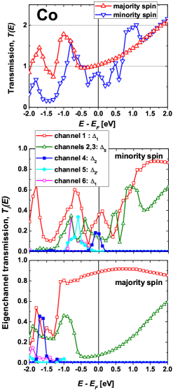
Figure 8: (Color online) Spin- and energy-dependent transmission decomposed to conduction eigenchannels for the Co single atom contact shown in Fig. 1.

Fig. 9 shows results for Pd. According to recent theoretical predictions Pd_wires monatomic Pd wires might exhibit magnetic properties. However, in this work we considered nonmagnetic solution, since a coordination number even for the contact atom was already big enough (Fig. 1) to suppress magnetism.Pd_wires Pd is isovalent to Ni. The Fermi level crosses the partially filled $d$ band. Therefore, the eigenchannel decomposition resembles the minority spin channels of Ni. However, due to a larger occupation number, transmission curves are shifted $\sim 0.5$ eV downwards in energy as compared with spin-down Ni modes. The conductance $G=1.41\,G_{0}$ is a sum of three channels. This value is in agreement with the conductance histogram of PdPd_hist which shows a broad maximum around $\simeq 1.7\,G_{0}$.

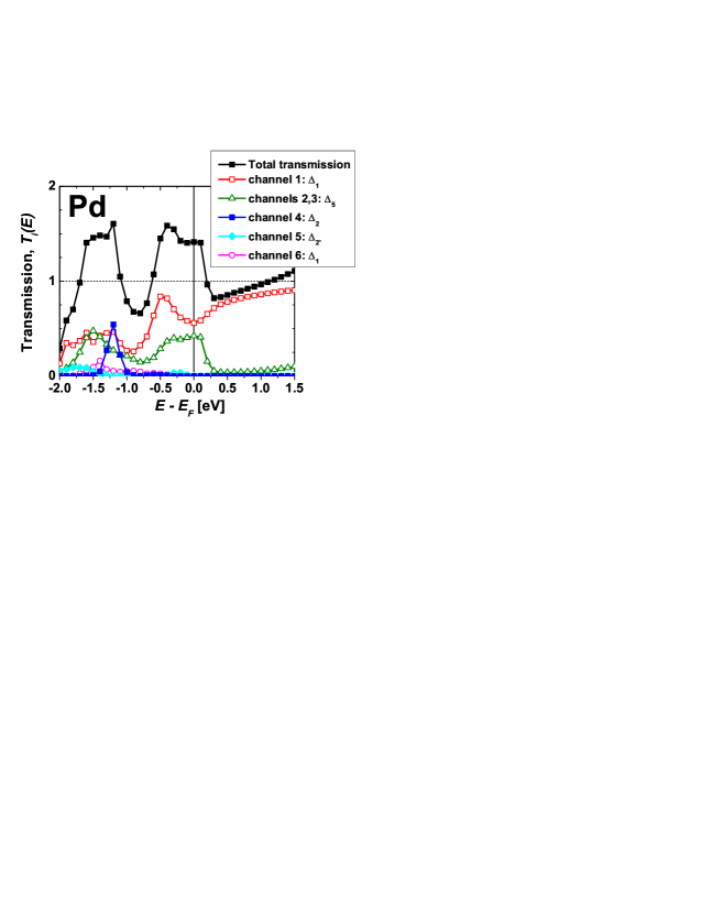
Figure 9: (Color online) Eigenchannel decomposition of the transmission for the Pd contact shown in Fig. 1.

We turn back to Ni and Co contacts and consider a situation when a relative orientation of magnetizations in the leads is antiparallel (AP), so that an abrupt atomic-scale domain wall is formed as shown in Table II. We see from Table I that, both for Ni and Co, the AP conductance reflects the structure of the minority spin channels and consists of a $\Delta_{1}$ and a $\Delta_{5}$ channel. For the atomic configuration shown in Fig. 1, we obtained ”optimistic” MR values: $-17\%$ in case of Ni, and $+23\%$ in case of Co, which are quite small in accordance with our previous study.PRB_MR However, the precise MR values as well as transmission curves for Co, differ from the results reported in our earlier work because of the different geometrical configurations of atomic contacts. The reason is that the transmission of $d$-like channels is quite sensitive to the exact geometry. PRB_MR We mention here, that a more accurate full-potential approach and an improved description of the electron correlations for localized $d$-electrons can somewhat affect presented results. That is also valid for the effects of atomic relaxations which were neglected. In particular, the exact values for the transmission probabilities and MR at the Fermi level reported in this study for different systems could be slightly changed. However, more precise calculations obviously will not affect the physical results of the present work.

Evident conclusions follow from presented examples. First, in contrast to earlier studies,Half_int_FM ; Half_int_exp the ferromagnetic Ni and Co contacts do not show any tendency to close one spin channel. On the contrary, both spin channels contribute to the conductance that gives only moderate magnetoresistance values. Independent of the geometry of the atomic contact the minority spin channel will include a sum of fractional contributions from many modes because the $d$ states are always present at the Fermi level. That agrees with later experiments by Untiedt et al.,Untiedt where the absence of conductance quantization for ferromagnetic Fe, Co and Ni contacts was clearly confirmed.

Second, an abrupt, atomic-scale domain wall pinned to the constriction does not show an impressive MR effect. For a fixed atomic configuration, the P and AP conductances are of the same order. Most likely, that more sophisticated calculations, involving relaxation effects and noncollinear magnetic moments in the domain wall, will not be able to change this statement.Tsymbal_PRL ; comment A recent researchCzerner towards transport in nanocontacts with noncollinear moments shows that energetically preferable noncollinear magnetic order results in a larger domain wall width as compared to the abrupt, collinear wall considered in the present paper. That leads to weakened scattering of electrons and a further reduction of the MR values.

Table 2: Spin magnetic moments (in $\mu_{B}$) at atoms forming Ni and Co contacts shown in Fig. 1 for the parallel (P) and the antiparallel (AP) orientation of magnetizations in the leads. Bulk magnetic moments are $0.62~{}\mu_{B}$ for Ni, and $1.62~{}\mu_{B}$ for Co.

	Ni		Co
Atom	P	AP	P	AP
Surface	$\phantom{+}0.66$	$\phantom{+}0.66$	$\phantom{+}1.78$	$\phantom{+}1.78$
Contact$-1$	$\phantom{+}0.70$	$\phantom{+}0.69$	$\phantom{+}1.83$	$\phantom{+}1.83$
1st contact	$\phantom{+}0.68$	$\phantom{+}0.54$	$\phantom{+}1.76$	$\phantom{+}1.64$
2nd contact	$\phantom{+}0.68$	$-0.54$	$\phantom{+}1.76$	$-1.64$
Contact$+1$	$\phantom{+}0.70$	$-0.69$	$\phantom{+}1.83$	$-1.83$
Surface	$\phantom{+}0.66$	$-0.66$	$\phantom{+}1.78$	$-1.78$

Coming to the experimental situation on ballistic magnetoresistance (BMR) effect in ferromagnetic contacts, we point out that large MR values Huge_MR_1 ; Hua_Chopra were usually measured for much thicker constrictions (as compared with atomic-sized contacts) with resistance in the range of hundreds of Ohms. It is believed,Magnetostriction1 ; Magnetostriction2 that such experiments suffer from many unavoidable artifacts induced by magnetomechanical effects that mimics the real MR signal which would come from the spin-polarized transport alone. However, recent studies by Sullivan et al.Sullivan_Ni and Chopra et al.Chopra_Co on Ni and Co atomic-sized contacts report BMR values in the range of $200\div 2000\%$ with discussion on the electronic origin of the effect due to domain wall scattering. Nevertheless attempts to minimize magnetostrictive effects were undertaken, we just can repeatMagnetostriction1 that a natural explanation of theseSullivan_Ni ; Chopra_Co and similar experiments Huge_MR ; Viret is that, due to magnetization reversal processes, unstable in time atomic constriction changes its contact area when magnetic field is applied. Characteristic steps and jumps in the measured field-dependent conductance (Fig. 4 of Ref. Sullivan_Ni, ) or resistance (Fig. 3a of Ref. Chopra_Co, , Fig. 3 of Ref. Viret, ) are distinct evidence of atomic reconstructions and fractional changes of the contact cross section. For example, just eliminating one contact atom from the configuration shown in Fig. 1 changes conductance of a Ni constriction from $1.2~{}G_{0}$ (chain of two atoms, see Table I) up to $\sim 2.8~{}G_{0}$ (one contact atom only, see Ref. Imp_Paper2, ), thus producing $\sim 130$% MR. Further increase of a contact area can give arbitrary high MR values, that supports hypothesis on mechanical nature of the effect.

VI Conclusions

To summarize, we have presented a formalism for the evaluation of conduction eigenchannels of metallic atomic-sized contacts from first-principles. We have combined the ab initio KKR Green’s function approach with the Kubo linear response theory. Starting from the scattering wave formulation of the conductance problem, we have built a special representation of the transmission matrix in terms of local, energy and angular momentum dependent basis inherent to the KKR method. We have proven that solutions of the eigenvalue problem for the obtained matrix are identical to conduction eigenchannels introduced by Landauer and Büttiker. Applications of the method have been presented by studying ballistic electron transport through Cu, Pd, Ni and Co single-atom contacts. The symmetry analysis of eigenchannels and its connection to the orbital classification known from the tight-binding approach were discussed in detail. Experiments on the electron transport through magnetic contacts were commented.

VII Acknowledgement

We acknowledge a financial support through the Deutsche Forschungsgemeinschaft (DFG), Priority Programme 1165: ”Nanowires and Nanotubes”.

Appendix A

We consider a practical implementation of the Kubo formula (9): positions $z=z_{\mathrm{L}}$ and $z^{\prime}=z_{\mathrm{R}}$ of the $S_{L}$ and $S_{R}$ planes are chosen within the semi-infinite electrodes, where $\Delta t$-matrix describing a scattering region is sufficiently small (for details, see Fig. 2). A sketch as how to find the conduction eigenchannels in this case has been given in Sec. IV.E. Below we complete that discussion by presenting a mathematical justification of the method.

We proceed in three steps: (i) since a position of $S_{L}$ and $S_{R}$ planes in Eq. (9) does not meet an asymptotic limit criterion, we expand the Green’s function in terms of scattering Bloch states in contrary to expansion (IV.3) involving unperturbed states; (ii) we use the Kubo formula (9) and express conductance as a trace of the appropriately defined current operator in $\boldsymbol{k}$-space; the obtained operator is identified with transmission matrix $\tau^{\dagger}\tau$; (iii) finally, we build up the equivalent site-angular momentum representation of the transmission matrix, that leads us to the required formulae [Eqs. (29), (30) of Sec. IV.E].

A.1 Expansion of the Green’s function.

To begin the proof, we note that the asymptotic representation (IV.3) of the Green’s function can be rewritten as

$$G^{+}(\mathbf{r},\mathbf{r^{\prime}},E)|_{z,z^{\prime}\to\mp\infty}$$

$$= -2\pi i\sum_{\boldsymbol{kk^{\prime}}}\overline{\Phi}_{\boldsymbol{k}}(\mathbf{r},E)\,{\left[\tau^{-1}(E)\right]_{\boldsymbol{kk^{\prime}}}}\ \Phi_{\boldsymbol{k^{\prime}}}(\mathbf{r^{\prime}},E)$$

where an expansion is performed over perturbed Bloch waves $\Phi_{\boldsymbol{k}}(\mathbf{r},E)=\Psi_{\boldsymbol{k}}(\mathbf{r},E)/\sqrt{v_{\boldsymbol{k}}}$ and $\overline{\Phi}_{\boldsymbol{k}}(\mathbf{r},E)=\overline{\Psi}_{\boldsymbol{\kappa}}(\mathbf{r},E)/\sqrt{v_{\boldsymbol{k}}}$ which were introduced in Sec. III. We remind, that function $\Phi_{\boldsymbol{k}}(\mathbf{r},E)$ is the solution of the Lippmann-Schwinger equation (III) associated with the in-coming unperturbed Bloch wave $\Psi^{\circ}_{\boldsymbol{k}}(\mathbf{r},E)/\sqrt{v_{\boldsymbol{k}}}$ in the left lead propagating towards atomic constriction ($v_{\boldsymbol{k}}\propto\mathrm{v}^{z}_{\boldsymbol{k}}>0$), while the second function, $\overline{\Phi}_{\boldsymbol{k}}(\mathbf{r},E)$, is the solution of the equation associated with the in-coming unperturbed Bloch wave $\Psi^{\circ\,*}_{\boldsymbol{k}}(\mathbf{r},E)/\sqrt{v_{\boldsymbol{-k}}}$ in the right lead ($v_{\boldsymbol{-k}}\propto\mathrm{v}^{z}_{\boldsymbol{-k}}<0$).

Consider now a general case, when $z=z_{\mathrm{L}}$ and $z^{\prime}=z_{\mathrm{R}}$ points related to planes $S_{L}$ and $S_{R}$ (see Fig. 2) are not taken infinitely far from atomic constriction. We note, that for the conductance evaluation one needs only the back-scattering term $\delta G^{+}(\mathbf{r},\mathbf{r^{\prime}},E)$ in Eq. (II), which is the solution of the Schrödinger equation without a source term. Therefore, we can expand $\delta G^{+}(\mathbf{r},\mathbf{r^{\prime}},E)$ over the eigenfunctions of the whole system corresponding to energy $E$. These are the propagating perturbed Bloch states,

$$\Psi_{\boldsymbol{k}}(\mathbf{r},E)=\sum_{nL}{\mathscr{C}}_{\boldsymbol{k},nL}(E)\,\phi_{L}(\mathbf{r}-\mathbf{R}_{n},E),$$ (32)

and the evanescent states,

$${\cal{X}}_{\alpha}(\mathbf{r},E)=\sum_{nL}{\Gamma}_{\alpha,nL}(E)\,\phi_{L}(\mathbf{r}-\mathbf{R}_{n},E),$$ (33)

where, in turn, both type of functions are expanded over atomic orbitals, and ${\mathscr{C}}_{\boldsymbol{k},nL}$ and ${\Gamma}_{\alpha,nL}$ are expansion coefficients.

In particular, matrix ${\mathscr{C}}_{\boldsymbol{\kappa},nL}$ is related to the matrix ${C}_{\boldsymbol{\kappa},nL}$ corresponding to the unperturbed Bloch waves (for details, see Ref. pert_BW, ):

$${\mathscr{C}}_{\boldsymbol{k},nL}(E)=\sum_{n^{\prime}L^{\prime}}\left[\bigl{\{}1-G_{0}(E)\,\Delta t(E)\bigr{\}}^{-1}\right]^{nn^{\prime}}_{LL^{\prime}}{C}_{\boldsymbol{k},n^{\prime}L^{\prime}}(E)$$

where the $\Delta t$-matrix describes the whole scattering region (a vacuum barrier plus an atomic constriction) and $G_{0}$ is the structural Green’s function of the three-dimensional periodic bulk crystal.

The evanescent states can be, for example, the surface states which are perturbed by an atomic constriction, as well as the states localized around impurities.

Both equations (32) and (33) can be joined to one matrix equation:

$$\left(\begin{array}[]{c}\Psi(\mathbf{r},E)\\ {\cal{X}}(\mathbf{r},E)\end{array}\right)=\left[\begin{array}[]{c}\mathscr{C}(E)\\ \Gamma(E)\end{array}\right]\phi(\mathbf{r},E),$$

where (…) stands for a column-vector, while […] denotes a matrix. We also expand the conjugated states as

$$\left(\begin{array}[]{c}\overline{\Psi}(\mathbf{r},E)\\ {\cal{X}}^{*}(\mathbf{r},E)\end{array}\right)=\left[\begin{array}[]{c}\widetilde{\mathscr{C}}(E)\\ \widetilde{\Gamma}(E)\end{array}\right]\phi(\mathbf{r},E).$$

We expand the back-scattering term $\delta G^{+}(\mathbf{r},\mathbf{r^{\prime}},E)$ over eigenfunctions $\Psi_{\boldsymbol{k}}(\mathbf{r},E)$ and ${\cal{X}}_{\alpha}(\mathbf{r},E)$ with energy $E$:

$$\delta G^{+}(\mathbf{r},\mathbf{r^{\prime}},E)\Bigl{|}_{\mathbf{r,r^{\prime}}\in S_{L,R}}$$

$$= \sum_{n\in S_{L},n^{\prime}\in S_{R}}\sum_{LL^{\prime}}\phi^{n}_{L}(\mathbf{r},E)\ G^{nn^{\prime}}_{LL^{\prime}}(E)\ \phi^{n^{\prime}}_{L^{\prime}}(\mathbf{r^{\prime}},E)$$

$$= \left(\begin{array}[]{c}\overline{\Psi}(\mathbf{r},E)\\ {\cal{X}}^{*}(\mathbf{r},E)\end{array}\right)^{T}\left[\begin{array}[]{cc}F^{00}(E)&F^{01}(E)\\ F^{10}(E)&F^{11}(E)\end{array}\right]\left(\begin{array}[]{c}\Psi(\mathbf{r^{\prime}},E)\\ {\cal{X}}(\mathbf{r^{\prime}},E)\end{array}\right)$$

$$= \phantom{+\ }\sum_{\boldsymbol{kk^{\prime}}}\overline{\Psi}_{\boldsymbol{k}}(\mathbf{r},E)\,F^{00}_{\boldsymbol{kk^{\prime}}}(E)\,\Psi_{\boldsymbol{k^{\prime}}}(\mathbf{r^{\prime}},E)$$

$$+\ \sum_{\boldsymbol{k}\beta}\overline{\Psi}_{\boldsymbol{k}}(\mathbf{r},E)\,F^{01}_{\boldsymbol{k}\beta}(E)\,{\cal{X}}_{\beta}(\mathbf{r^{\prime}},E)$$

$$+\ \sum_{\alpha\boldsymbol{k^{\prime}}}{\cal{X}}^{*}_{\alpha}(\mathbf{r},E)\,F^{10}_{\alpha\boldsymbol{k^{\prime}}}(E)\,\Psi_{\boldsymbol{k^{\prime}}}(\mathbf{r^{\prime}},E)$$

$$+\ \sum_{\alpha\beta}{\cal{X}}^{*}_{\alpha}(\mathbf{r},E)\,F^{11}_{\alpha\beta}(E)\,{\cal{X}}_{\beta}(\mathbf{r},E)$$

$$= \delta G_{+}^{(1)}(\mathbf{r},\mathbf{r^{\prime}},E)+\delta G_{+}^{(2)}(\mathbf{r},\mathbf{r^{\prime}},E).$$ (41)

Only the first term

$$\delta G_{+}^{(1)}(\mathbf{r},\mathbf{r^{\prime}},E)=\sum_{\boldsymbol{kk^{\prime}}}\overline{\Psi}_{\boldsymbol{k}}(\mathbf{r},E)\,F^{00}_{\boldsymbol{kk^{\prime}}}(E)\,\Psi_{\boldsymbol{k^{\prime}}}(\mathbf{r^{\prime}},E)$$ (42)

exists in the asymptotic case, while other three terms, denoted as $\delta G_{+}^{(2)}(\mathbf{r},\mathbf{r^{\prime}},E)$, contain contributions of the evanescent states which decay within the leads.

The unknown matrix $F=\{F^{ij}\}$ in Eq. (41) satisfies the equation (below we will skip for simplicity the obvious energy dependence):

$$\left[\widetilde{\mathscr{C}}^{T}\ \widetilde{\Gamma}^{T}\right]\times\left[\begin{array}[]{cc}F^{00}&F^{01}\\ F^{10}&F^{11}\end{array}\right]\times\left[\begin{array}[]{c}{\mathscr{C}}\\ \Gamma\end{array}\right]=G_{\mathrm{LR}},$$

where symbol $T$ denotes transpose, and matrix $G_{\mathrm{LR}}$ is introduced which contains selected matrix elements of the structural Green’s function $G_{LL^{\prime}}^{nn^{\prime}}$ with $n\in S_{\mathrm{L}}$ and $n^{\prime}\in S_{\mathrm{R}}$.

To find matrices $F^{ij}$, we introduce the block-matrix $\left[{\cal{B}}^{\dagger}\ \Delta^{\dagger}\right]$ which is a solution of the following equation (here symbol $\dagger$ denotes Hermitian conjugate):

$$\left[\begin{array}[]{c}{\mathscr{C}}\\ \Gamma\end{array}\right]\times\left[{\cal{B}}^{\dagger}\ \Delta^{\dagger}\right]=\left[\begin{array}[]{cc}{\mathscr{C}}{\cal{B}}^{\dagger}&{\mathscr{C}}\Delta^{\dagger}\\ \Gamma{\cal{B}}^{\dagger}&\Gamma\Delta^{\dagger}\end{array}\right]=\left[\begin{array}[]{cc}1&0\\ 0&1\end{array}\right].$$ (43)

This means, that matrix $\left[{\cal{B}}^{\dagger}\ \Delta^{\dagger}\right]$ is the inverse or (in general case) the pseudoinverse Gantmacher matrix to the matrix with ${\mathscr{C}}$- and $\Gamma$-blocks.BD_matrix .

The equation similar to Eq. (43) exists for other matrices:

$$\left[\begin{array}[]{c}\widetilde{\cal{B}}^{*}\\ \widetilde{\Delta}^{*}\end{array}\right]\times\left[\widetilde{\mathscr{C}}^{T}\ \widetilde{\Gamma}^{T}\right]=\left[\begin{array}[]{cc}\widetilde{\cal{B}}^{*}\,\widetilde{\mathscr{C}}^{T}&\widetilde{\cal{B}}^{*}\,\widetilde{\Gamma}^{T}\\ \widetilde{\Delta}^{*}\,\widetilde{\mathscr{C}}^{T}&\widetilde{\Delta}^{*}\,\widetilde{\Gamma}^{T}\end{array}\right]=\left[\begin{array}[]{cc}1&0\\ 0&1\end{array}\right],$$ (44)

where symbol $*$ denotes complex conjugate of the matrix elements only.

With the use of Eqs. (43), (44) we find solution for $F=\{F^{ij}\}$:

$$\left[\begin{array}[]{cc}F^{00}&F^{01}\\ F^{10}&F^{11}\end{array}\right]=\left[\begin{array}[]{cc}\widetilde{\cal{B}}^{*}G_{\mathrm{LR}}{\cal{B}}^{\dagger}&\widetilde{\cal{B}}^{*}G_{\mathrm{LR}}{\Delta}^{\dagger}\\ \widetilde{\Delta}^{*}G_{\mathrm{LR}}{\cal{B}}^{\dagger}&\widetilde{\Delta}^{*}G_{\mathrm{LR}}{\Delta}^{\dagger}\end{array}\right],$$

Then expansion coefficients of the $\delta G^{(1)}_{+}$ term read as

$$F^{00}_{\boldsymbol{kk^{\prime}}}(E)$$

$$= \sum_{n\in S_{\mathrm{L}},n^{\prime}\in S_{\mathrm{R}}}\sum_{LL^{\prime}}\widetilde{\cal{B}}^{*}_{\boldsymbol{k},nL}(E)\bigl{[}G_{\mathrm{LR}}(E)\bigr{]}^{nn^{\prime}}_{LL^{\prime}}{\cal{B}}^{\dagger}_{n^{\prime}L^{\prime},\boldsymbol{k^{\prime}}}(E).$$

With help of matrix $\tau^{-1}_{\mathrm{LR}}(E)$,

$$\left[\tau^{-1}_{\mathrm{\,LR}}(E)\right]_{\boldsymbol{kk^{\prime}}}=-\sqrt{v_{\boldsymbol{\kappa}}}\ \frac{F^{00}_{\boldsymbol{kk^{\prime}}}(E)}{2\pi i}\ \sqrt{v_{\boldsymbol{\kappa^{\prime}}}}$$ (45)

(with positive velocities under square-roots) we write down Eq. (42) as

$$\delta G_{+}^{(1)}(\mathbf{r},\mathbf{r^{\prime}},E)\Bigl{|}_{\mathbf{r,r^{\prime}}\in S_{L,R}}$$

$$= -2\pi i\sum_{\boldsymbol{kk^{\prime}}}\overline{\Phi}_{\boldsymbol{k}}(\mathbf{r},E)\,\left[\tau^{-1}_{\mathrm{\,LR}}(E)\right]_{\boldsymbol{kk^{\prime}}}\Phi_{\boldsymbol{k^{\prime}}}(\mathbf{r^{\prime}},E).$$

Comparing obtained equation with one for the asymptotic limit [Eq. (A.1)] and taking into account that in fact $\tau^{-1}_{\mathrm{LR}}(E)$ is independent on the positions of the L and R planes, we obtain:

$$\left[\tau^{-1}_{\mathrm{LR}}(E)\right]_{\boldsymbol{kk^{\prime}}}=\left[\tau^{-1}(E)\right]_{\boldsymbol{kk^{\prime}}}.$$ (47)

A.2 Evaluation of conductance

When conductance is evaluated, only $\delta G^{(1)}_{+}(\mathbf{r},\mathbf{r}^{\prime},E)$ term in expansion (41) contributes. Other term, $\delta G^{(2)}_{+}(\mathbf{r},\mathbf{r^{\prime}},E)$, contains the evanescent states which decay within the leads and, therefore, have zero velocities along the current flow. When Eq. (A.1) is inserted into the Kubo formula (9) we obtain:

$$g=g_{0}\sum_{\boldsymbol{kk^{\prime}}}\sum_{\boldsymbol{k_{1}k^{\prime}_{1}}}{\cal{J}}^{\mathrm{L}}_{\boldsymbol{k_{1}k}}\left[\frac{1}{\tau_{\mathrm{LR}}}\right]_{\boldsymbol{kk^{\prime}}}{\cal{J}}^{\mathrm{R}}_{\boldsymbol{k^{\prime}k^{\prime}_{1}}}\left[\frac{1}{\tau^{\dagger}_{\mathrm{RL}}}\right]_{\boldsymbol{k^{\prime}_{1}k_{1}}},$$ (48)

where all matrices are evaluated at the Fermi energy ($E_{F}=E_{\boldsymbol{k}}=E_{\boldsymbol{k^{\prime}}}=\dots$). Here we have introduced the current operators related to the left (L) lead,

$${\cal{J}}^{\mathrm{L}}_{\boldsymbol{kk^{\prime}}}(E)$$

$$= 2\pi\int\limits_{S_{\mathrm{L}}}dS\left[\overline{\Phi}^{\,*}_{\boldsymbol{k}}(\mathbf{r},E)\,i\!\stackrel{{\scriptstyle\leftrightarrow}}{{\partial_{z}}}\overline{\Phi}_{\boldsymbol{k^{\prime}}}(\mathbf{r},E)\right]\ =\ \bigl{[}\tau^{\dagger}\tau\bigr{]}_{\boldsymbol{kk^{\prime}}},$$

and to the right (R) one:

$${\cal{J}}^{\mathrm{R}}_{\boldsymbol{kk^{\prime}}}(E)$$

$$= 2\pi\int\limits_{S_{\mathrm{R}}}dS\left[\Phi_{\boldsymbol{k}}(\mathbf{r},E)\,i\!\stackrel{{\scriptstyle\leftrightarrow}}{{\partial_{z}}}\Phi^{\,*}_{\boldsymbol{k^{\prime}}}(\mathbf{r},E)\right]\ =\ \bigl{[}\tau\tau^{\dagger}\bigr{]}_{\boldsymbol{kk^{\prime}}},$$

where basis $\nu$ of eigenchannels (see Sec. III) was used to evaluate the matrix elements. With help of (A.2) and (A.2), equation (48) for conductance $g$ takes a form:

$$g = g_{0}\mathrm{Tr}_{\boldsymbol{k}}\left(\tau^{\dagger}\tau\,{\cal{O}}^{\mathrm{\,LR}}\right)$$

$$= g_{0}\mathrm{Tr}_{\boldsymbol{k}}\left(\tau^{\dagger}\tau\right)\ =\ g_{0}\mathrm{Tr}_{\boldsymbol{k}}\left({\cal{J}}^{\mathrm{L}}\right),$$

where ${\cal{O}}^{\mathrm{\,LR}}_{\boldsymbol{kk^{\prime}}}=\delta_{\boldsymbol{kk^{\prime}}}$ is the unitary operator in the $\boldsymbol{k}$-space:

$${\cal{O}}^{\mathrm{\,LR}} = \tau^{-1}_{\mathrm{LR}}\,{\cal{J}}^{\mathrm{R}}\,\bigl{(}\tau^{\dagger}_{\mathrm{RL}}\bigr{)}^{-1}$$

$$= \tau^{-1}_{\mathrm{LR}}\bigl{(}\tau\tau^{\dagger}\bigr{)}\bigl{(}\tau^{\dagger}_{\mathrm{RL}}\bigr{)}^{-1}=1,$$

and Eqs. (47) and (A.2) were used.

When the perturbed Bloch waves are expanded over atomic orbitals,

$$\Phi_{\boldsymbol{\kappa}}(\mathbf{r},E) = \frac{1}{\sqrt{v_{\boldsymbol{k}}}}\ \Psi_{\boldsymbol{k}}(\mathbf{r},E)$$

$$= \frac{1}{\sqrt{2\pi}}\sum_{n\in S_{R}}\sum_{L}{X}_{\boldsymbol{k},nL}(E)\,\phi^{n}_{L}(\mathbf{r},E),$$

$$\overline{\Phi}_{\boldsymbol{k}}(\mathbf{r},E) = \frac{1}{\sqrt{v_{\boldsymbol{k}}}}\ \overline{\Psi}_{\boldsymbol{k}}(\mathbf{r},E)$$

$$= \frac{1}{\sqrt{2\pi}}\sum_{n\in S_{L}}\sum_{L}\widetilde{X}_{\boldsymbol{k},nL}(E)\,\phi^{n}_{L}(\mathbf{r},E),$$

current operators ${\cal{J}}^{\mathrm{L}}$ and ${\cal{J}}^{\mathrm{R}}$ take a form (energy dependence is skipped):

$${\cal{J}}^{\mathrm{L}}_{\boldsymbol{kk^{\prime}}} = \sum_{nn^{\prime}\in S_{L}}\sum_{LL^{\prime}}\widetilde{X}^{*}_{\boldsymbol{k},nL}\left[D_{\mathrm{L}}\right]^{nn^{\prime}}_{LL^{\prime}}\widetilde{X}^{*\dagger}_{n^{\prime}L^{\prime},\boldsymbol{k^{\prime}}},$$ (53)

$${\cal{J}}^{\mathrm{R}}_{\boldsymbol{kk^{\prime}}} = \sum_{nn^{\prime}\in S_{R}}\sum_{LL^{\prime}}{X}_{\boldsymbol{k},nL}\left[D_{\mathrm{R}}\right]^{nn^{\prime}}_{LL^{\prime}}{X}^{\dagger}_{n^{\prime}L^{\prime},\boldsymbol{k^{\prime}}},$$

where operators $X$ and $\widetilde{X}$ are defined as

$${X}_{\boldsymbol{k},nL}(E) = \left(\frac{2\pi}{v_{\boldsymbol{k}}}\right)^{1/2}{\mathscr{C}}_{\boldsymbol{k},nL}(E),$$ (54)

$$\widetilde{X}_{\boldsymbol{k},nL}(E) = \left(\frac{2\pi}{v_{\boldsymbol{k}}}\right)^{1/2}\widetilde{\mathscr{C}}_{\boldsymbol{k},nL}(E),$$

and operators $D_{\mathrm{L}}$ and $D_{\mathrm{R}}$ were introduced in Eq. (IV.4).

A.3 Decomposition of current operator

According to Eq. (A.2) conductance is determined by operator $\cal{J}^{\mathrm{L}}=\tau^{\dagger}\tau$. The formal representation (53) of the current operator $\cal{J}^{\mathrm{L}}$ in $\boldsymbol{k}$-space is not suitable for practical implementation. It can be used, however, to find an equivalent representation in $(n,L)$-space. Using (53) together with representation of operator $D_{\mathrm{L}}$ [Eqs. (23), (24)] we can decompose $\cal{J}^{\mathrm{L}}$ in two terms:

$${\cal{J}}^{\mathrm{L}}={\cal{J}}^{(+)}_{\mathrm{L}}+{\cal{J}}^{(-)}_{\mathrm{L}},$$ (55)

where

$${\cal{J}}^{(+)}_{\mathrm{L}}=+\widetilde{X}^{*}\,U_{\mathrm{L}}\left(\begin{array}[]{cc}\Delta^{+}_{\mathrm{L}}&0\\ 0&0\end{array}\right)U_{\mathrm{L}}^{\dagger}\,\bigl{[}\widetilde{X}^{*}\bigr{]}^{\dagger}$$ (56)

has only positive (non-negative) eigenvalues, while

$${\cal{J}}^{(-)}_{\mathrm{L}}=-\widetilde{X}^{*}\,U_{\mathrm{L}}\left(\begin{array}[]{cc}0&0\\ 0&\Delta^{-}_{\mathrm{L}}\end{array}\right)U_{\mathrm{L}}^{\dagger}\,\bigl{[}\widetilde{X}^{*}\bigr{]}^{\dagger}$$ (57)

has only negative (or zero-) eigenvalues, and $\Delta_{\mathrm{L}}^{\pm}$ are diagonal matrices with nonnegative elements [Eqs. (23), (24)]. The advantage of operators $\cal{J}^{(\pm)}_{\mathrm{L}}$ over operator $\cal{J}_{\mathrm{L}}$ is that matrices $\Delta^{\pm}_{\mathrm{L}}$ are positive definite, while anti-symmetric matrix $D_{\mathrm{L}}$ is not. As we show below in Appendix B, that makes possible to find for operators ${\cal{J}}^{(\pm)}_{\mathrm{L}}$ an equivalent, site-angular momentum $(n,L)$ representation, while it is not the case for full operator ${\cal{J}}_{\mathrm{L}}$. We mention also, that in the asymptotic limit the contribution due to ${\cal{J}}^{(-)}_{\mathrm{L}}$ vanishes. However, in general case, spectra of both operators should be found.

To clarify these ideas, let us elucidate a physical meaning of Eq. (55). Consider new basis functions in $(n,L)$-space which are constructed with help of unitary matrix $U_{\mathrm{L}}$,

$$\chi_{\alpha}(\mathbf{r},E)=\sum_{n\in S_{L}}\sum_{L}\phi^{n}_{L}(\mathbf{r},E)\,\bigl{[}U_{\mathrm{L}}(E)\bigr{]}_{nL,\alpha},$$

so that the velocity operator $D_{\mathrm{L}}=U_{L}D^{0}_{\mathrm{L}}U^{\dagger}_{L}$ in $(n,L)$-space introduced in Eq. (21) is diagonal in the new basis:

$$\bigl{[}D_{\mathrm{L}}^{0}(E)\bigr{]}_{\alpha\beta}$$

$$= \int_{S_{\mathrm{L}}}dS\left[\chi^{*}_{\alpha}(\mathbf{r},E)\,i\!\stackrel{{\scriptstyle\leftrightarrow}}{{\partial_{z}}}\chi_{\beta}(\mathbf{r},E)\right]\ =\ \delta^{\circ}_{\alpha}(E)\,\delta_{\alpha\beta}.$$

Let us examine further the wave function $\overline{\Phi}_{\boldsymbol{k}}(\mathbf{r},E)$ which defines the current operator ${\cal{J}}^{\mathrm{L}}$ [Eq. (A.2)]. This function is the solution of the Lippmann-Schwinger equation associated with the in-coming unperturbed Bloch wave $\Phi^{\circ\,*}_{\boldsymbol{\kappa}}(\mathbf{r},E)$ (initial channel) propagating from the right (R) lead towards the nanocontact and being scattered on it. Within the left (L) lead ($\mathbf{r}\in S_{\mathrm{L}}$) we have:

$$\overline{\Phi}_{\boldsymbol{k}}(\mathbf{r},E)\ =\ \overline{\Phi}^{\,(+)}_{\boldsymbol{k}}(\mathbf{r},E)\ +\ \overline{\Phi}^{\,(-)}_{\boldsymbol{k}}(\mathbf{r},E),$$

where

$$\overline{\Phi}^{\,(\pm)}_{\boldsymbol{k}}(\mathbf{r},E)=\frac{1}{\sqrt{2\pi}}\sum_{\alpha^{\pm}}\chi_{\alpha}(\mathbf{r},E)\,\bigl{(}\widetilde{X}^{*}U_{\mathrm{L}}\bigr{)}^{\dagger}_{\alpha\boldsymbol{k}},$$ (59)

here the ($\alpha^{\pm}$)-sums run over the half of the indices of the basis functions $\chi_{\alpha}(\mathbf{r},E)$, corresponding either to the ”positive” or to the ”negative” window of the spectrum. Thus, the wave function $\overline{\Phi}_{\boldsymbol{k}}(\mathbf{r},E)$ in the L lead is a linear combination of two functions. The first one, $\overline{\Phi}^{(+)}_{\boldsymbol{k}}(\mathbf{r},E)$ carries the flux in the initial direction of the in-coming wave with momentum $\boldsymbol{-k}$, from the L electrode to the R one. The second function, $\overline{\Phi}^{(-)}_{\boldsymbol{k}}(\mathbf{r},E)$, carries the flux in the direction being opposite to the propagation direction of the in-coming wave. An example illustrating this idea for free electrons is shown in Fig. 3.

One can check, that operator ${\cal{J}}_{\mathrm{L}}^{(+)}$ is defined on functions $\overline{\Phi}^{(+)}_{\boldsymbol{k}}(\mathbf{r},E)$ only, while ${\cal{J}}_{\mathrm{L}}^{(-)}$ is defined on $\overline{\Phi}^{(-)}_{\boldsymbol{\kappa}}(\mathbf{r},E)$:

$$\bigl{[}{\cal{J}}_{\mathrm{L}}^{(\pm)}(E)\bigr{]}_{\boldsymbol{kk^{\prime}}}=2\pi\int\limits_{S_{L}}dS\left[\overline{\Phi}^{(\pm)\,*}_{\boldsymbol{k}}(\mathbf{r},E)\,i\!\stackrel{{\scriptstyle\leftrightarrow}}{{\partial_{z}}}\overline{\Phi}^{(\pm)}_{\boldsymbol{k^{\prime}}}(\mathbf{r},E)\right],$$

because, according to Eqs. (A.3) and (59), the cross-terms involving both functions, $\overline{\Phi}^{(+)}_{\boldsymbol{k}}(\mathrm{r},E)$ and $\overline{\Phi}^{(-)}_{\boldsymbol{k}}(\mathrm{r},E)$, vanish.

Obviously, that if the $S_{\mathrm{L}}$ plane is chosen way behind the scattering region, the $\overline{\Phi}^{(-)}_{\boldsymbol{k}}(\mathbf{r},E)$ turns to zero and the contribution due to $\cal{J}_{\mathrm{L}}^{(-)}$ vanishes. In general case, both operators, $\cal{J}^{(+)}_{\mathrm{L}}$ and $\cal{J}^{(-)}_{\mathrm{L}}$, should be considered.

A.4 Spectrum of current operators.

In this section we show that transmission probability of the conduction eigenchannel $\nu$ is given by $T_{\nu}=\tau_{\nu}^{+}-\tau_{\nu}^{-}$, where $\tau_{\nu}^{+}$ and $(-\tau_{\nu}^{-})$ are positive and negative eigenvalues of operators ${\cal{J}}^{(+)}_{\mathrm{L}}$ and ${\cal{J}}^{(-)}_{\mathrm{L}}$, respectively.

Assume, that we know matrix $\theta$ (introduced in Sec.III) which is the unitary transform to the basis of eigenchannels. According to Ref. conjphi, we have:

$$\overline{\Phi}_{\nu}(\mathbf{r},E) = \sum_{\boldsymbol{k}}\overline{\Phi}_{\boldsymbol{k}}(\mathbf{r},E)\,\theta^{\dagger}_{\boldsymbol{k}\nu}(E)$$

$$= \overline{\Phi}_{\nu}^{(+)}(\mathbf{r},E)+\overline{\Phi}_{\nu}^{(-)}(\mathbf{r},E).$$

Thus, we have decomposed the wave function of each eigenchannel in two terms: $\overline{\Phi}_{\nu}^{(\pm)}=\sum_{\boldsymbol{k}}\overline{\Phi}^{\,(\pm)}_{\boldsymbol{k}}\,\theta^{\dagger}_{\boldsymbol{k}\nu}$.

Consider further the transmission matrix $T$ in the basis of eigenchannels:

$$T_{\nu\mu} = T_{\nu}\delta_{\nu\mu}\ =\ \left[\theta(\tau^{\dagger}\tau)\theta^{\dagger}\right]_{\nu\mu}$$

$$= 2\pi\int_{S_{\mathrm{L}}}dS\ \left[\overline{\Phi}_{\nu}^{\,*}(\mathbf{r},E)\ i\!\stackrel{{\scriptstyle\leftrightarrow}}{{\partial_{z}}}\overline{\Phi}_{\mu}(\mathbf{r},E)\right]$$

$$= T^{(+)}_{\nu\mu}+T^{(-)}_{\nu\mu},$$

with

$$T^{(\pm)}_{\nu\mu}=2\pi\int_{S_{\mathrm{L}}}dS\ \left[\overline{\Phi}_{\nu}^{(\pm)\,*}(\mathbf{r},E)\,i\!\stackrel{{\scriptstyle\leftrightarrow}}{{\partial_{z}}}\overline{\Phi}^{(\pm)}_{\mu}(\mathbf{r},E)\right].$$

Operators $T^{(\pm)}$ are related to current operators ${\cal{J}}^{(\pm)}_{\mathrm{L}}$ via the unitary transform $\theta$: $T^{(\pm)}=\theta{\cal{J}}_{\mathrm{L}}^{(\pm)}\theta^{\dagger}$.

The unitary transform $\theta$ diagonalizes the full operator ${\cal{J}}^{\mathrm{L}}={\cal{J}}^{(+)}_{\mathrm{L}}+{\cal{J}}^{(-)}_{\mathrm{L}}$. Using the representation (53) of operators ${\cal{J}}^{(\pm)}_{\mathrm{L}}$ we can check, that ${\cal{J}}^{(+)}_{\mathrm{L}}$ and ${\cal{J}}^{(-)}_{\mathrm{L}}$ do not commutate. Thus, the $T^{(\pm)}$ operators do not have a diagonal form in the basis of eigenchannels. Therefore, we represent each of these operators as sum of diagonal and off-diagonal terms:

$$T^{(-)}_{\nu\mu} = \stackrel{{\scriptstyle\circ}}{{T}}^{(-)}_{\nu\mu}\ +\ \delta T^{(-)}_{\nu\mu},$$ (60)

$$T^{(+)}_{\nu\mu} = \stackrel{{\scriptstyle\circ}}{{T}}^{(+)}_{\nu\mu}\ -\ \delta T^{(-)}_{\nu\mu},$$

here $\delta T^{(-)}_{\nu\nu}=0$, and off-diagonal contributions are of different signs because the sum of two matrices is the diagonal matrix $T_{\nu}\delta_{\mu\nu}$. The diagonal terms are

$$\stackrel{{\scriptstyle\circ}}{{T}}^{(+)}_{\nu\mu}\ =\ \tau^{+}_{\nu}\delta_{\nu\mu},\quad\stackrel{{\scriptstyle\circ}}{{T}}^{(-)}_{\nu\mu}=-\tau^{-}_{\nu}\delta_{\nu\mu},$$ (61)

where

$$\tau^{\pm}_{\nu}\ =\ 2\pi\int_{S_{\mathrm{L}}}dS\ \left[\overline{\varPhi}_{\nu}^{(\pm)\,*}(\mathbf{r},E)\,i\!\stackrel{{\scriptstyle\leftrightarrow}}{{\partial_{z}}}\overline{\varPhi}^{(\pm)}_{\nu}(\mathbf{r},E)\right].$$

and transmission probability of the eigenchannel is given by $T_{\nu}=\tau^{+}_{\nu}-\tau^{-}_{\nu}$. Here the first term arises due to all multiple scattering contributions in the direction of the current, while the second term is due to scattering contributions in the opposite direction.

In spite of the fact that operators $T^{(+)}$ and $T^{(-)}$ can not be diagonalized within the unique unitary transform, one can show that off-diagonal terms $\delta T^{(-)}_{\nu\mu}\neq 0$ are small. They are determined by functions $\overline{\Phi}^{(-)}_{\nu}(\mathbf{r},E)$ with negative velocities with respect to the initial velocity of the in-coming channel $\nu$ incident from the right (R) lead. The function $\overline{\Phi}^{(-)}_{\nu}(\mathbf{r},E)$ in the left (L) lead is small as compared with $\overline{\Phi}^{(+)}_{\nu}(\mathbf{r},E)$. When the $S_{\mathrm{L}}$ plane is placed far enough from the surface, the $\overline{\Phi}^{(-)}_{\nu}(\mathbf{r},E)$ collects all multiple scattering events in the opposite direction to the current flow. However, such scattering processes are possible only due to small inhomogeneities of the potential which is not exactly the bulk one around $z_{\mathrm{L}}$ (see Fig. 3). Thus, we can write down:

$$\bigl{|}\overline{\Phi}^{(-)}_{\nu}(\mathbf{r},E)\bigr{|}\ \sim\ \rho\,\bigl{|}\overline{\Phi}^{(+)}_{\nu}(\mathbf{r},E)\bigr{|},$$

where parameter $\rho<1$ has a meaning of reflection amplitude (see caption of Fig. 3). The $\rho^{2}$ is of the order of reflection probability, which (in realistic calculations) is $\rho^{2}\sim\tau^{-}_{\nu}/\tau^{+}_{\nu}\sim 0.1$. Thus, off-diagonal terms, $\delta T^{(-)}_{\mu\nu}$, contain small parameter $\lambda\sim\rho^{2}\sim 0.1$. Since $\delta T^{(-)}_{\mu\mu}=0$, according to the perturbation theory QM the difference between eigenvalues of operators $T^{(\pm)}_{\mu\nu}$ [Eq.(60)] and $\stackrel{{\scriptstyle\circ}}{{T}}^{(\pm)}_{\nu\mu}$ [Eq.(61)] appears only in the second order, which is $O(\lambda^{2})\sim 0.01$. Therefore, the operators ${\cal{J}}^{(\pm)}_{\mathrm{L}}$ provide a feasible way to find $\tau^{(\pm)}_{\nu}$ with good enough precision.

To find the spectrum of positive definite operators ${\cal{J}}_{\mathrm{L}}^{(\pm)}$ we represent them in the form $\Sigma_{\pm}^{\dagger}\Sigma_{\pm}$, where $\Sigma_{\pm}$ maps the site-orbital space on the $\boldsymbol{k}$-space. We can prove (see Appendix B) that spectrum of $\Sigma^{\dagger}_{\pm}\Sigma_{\pm}$ is the same as for operator $\Sigma_{\pm}\Sigma^{\dagger}_{\pm}$ which is defined in $(n,L)$-space and reads as

$${\cal{T}}^{(\pm)}=\pm\left(\pm D^{\pm}_{\mathrm{L}}\right)^{1/2}\bigl{[}\widetilde{X}^{*}\bigr{]}^{\dagger}{\cal{O}}^{\,\mathrm{LR}}\widetilde{X}^{*}\left(\pm D^{\pm}_{\mathrm{L}}\right)^{1/2}.$$

Here we have used the unit operator in $\boldsymbol{k}$-space ${\cal{O}}^{\,\mathrm{LR}}=\tau^{-1}_{\mathrm{LR}}\,{\cal{J}}_{\mathrm{R}}\bigl{(}\tau^{\dagger}_{\mathrm{RL}}\bigr{)}^{-1}=\delta_{\boldsymbol{kk^{\prime}}}$ introduced in Eq. (A.2). By using equations (45), (A.2), (53), (54), we obtain expression for operator ${\cal{T}}^{(\pm)}$:

$${\cal{T}}^{(\pm)}$$

$$= \pm\left(\pm D^{\pm}_{\mathrm{L}}\right)^{1/2}\bigl{[}\widetilde{X}^{*}\bigr{]}^{\dagger}\left[\tau^{-1}_{\mathrm{LR}}\,{\cal{J}}_{\mathrm{R}}\bigl{(}\tau^{\dagger}_{\mathrm{RL}}\bigr{)}^{-1}\right]\widetilde{X}^{*}\left(\pm D^{\pm}_{\mathrm{L}}\right)^{1/2}$$

$$= \pm\left(\pm D^{+}_{\mathrm{L}}\right)^{1/2}\bigl{[}\widetilde{\mathscr{C}}^{*}\bigr{]}^{\dagger}\left(\widetilde{\cal{B}}^{*}\,G_{\mathrm{LR}}\,{\cal{B}}^{\dagger}\right)\mathscr{C}\,D_{\mathrm{R}}\,{\mathscr{C}}^{\dagger}$$

$$\times\left({\cal{B}}\,G^{\dagger}_{\mathrm{RL}}\,[\widetilde{\cal{B}}^{*}]^{\dagger}\right)\widetilde{\mathscr{C}}^{*}\left(\pm D^{\pm}_{\mathrm{L}}\right)^{1/2}$$

$$= \pm\left(\pm D^{\pm}_{\mathrm{L}}\right)^{1/2}\,G_{\mathrm{LR}}\,D_{\mathrm{R}}G^{\dagger}_{\mathrm{RL}}\left(\pm D^{\pm}_{\mathrm{L}}\right)^{1/2},$$

where orthogonality relationcalBC ${\cal{B}}^{\dagger}\mathscr{C}=[\widetilde{\cal{B}}^{*}]^{\dagger}\widetilde{\cal{C}}^{*}=1$ was used. Thus, we come to Eq. (30) of Sec. VI.

Appendix B

Let us consider operator $\Lambda_{\boldsymbol{kk^{\prime}}}(E)$ acting in $\boldsymbol{k}$-space of a following kind:

$$\Lambda=X\Delta X^{\dagger},$$

where $\Delta$ is a positive definite hermitian operator acting in the site-orbital $(n,L)$-space. Let $\Theta_{\nu\boldsymbol{k}}$ be a unitary transform which diagonalizes operator $\Lambda$,

$$\Theta\Lambda\Theta^{\dagger}=\mbox{diag}\{\Lambda_{\nu}\}=\hat{\Lambda}_{0}.$$

Our goal is to find a spectrum of $\Lambda$ with help of $(n,L)$-space. Following Sec.III, we represent $\Lambda$ in the form:

$$\Lambda=\Sigma^{\dagger}\Sigma=X\Delta X^{\dagger},$$

with $\Sigma=\Delta^{1/2}X^{\dagger}$ and $\Sigma^{\dagger}=X\Delta^{1/2}$. A square-root from the positive definite hermitian operator is defined as

$$\Delta^{1/2}=({\Delta}^{1/2})^{\dagger}=U\Delta_{0}^{1/2}\,U^{\dagger},$$

where the unitary matrix $U$ transforms $\Delta$ to the diagonal form $\Delta_{0}=U^{\dagger}\,\Delta\,U$.

Let us show that a spectrum of operator $\Lambda=\Sigma^{\dagger}\Sigma$ acting in the $\boldsymbol{k}$-space, is the same as a spectrum of operator $\Sigma\Sigma^{\dagger}$ acting in the $(n,L)$-space. Let $\Omega$ be such matrix that

$$\Theta\Sigma^{\dagger}\Omega^{\dagger}=\Omega\Sigma\Theta^{\dagger}=\mbox{diag}\{\sqrt{\Lambda_{\nu}}\}=\hat{\lambda}_{0}.$$

Solution for $\Omega$ is $\Omega_{\nu,nL}=\sum_{\boldsymbol{k}}\mbox{diag}\{1/\sqrt{\Lambda_{\nu}}\}\Theta_{\nu\boldsymbol{k}}\Sigma^{\dagger}_{\boldsymbol{k},nL}$. Matrix $\Omega$ diagonalizes $\Sigma\Sigma^{\dagger}$:

$$\Omega(\Sigma\Sigma^{\dagger})\Omega^{\dagger} = \hat{\lambda}_{0}^{-1}\Theta\Sigma^{\dagger}\,(\Sigma\Sigma^{\dagger})\,\Sigma\Theta^{\dagger}\hat{\lambda}^{-1}_{0}$$

$$= \hat{\lambda}_{0}^{-1}\,(\Theta\Sigma^{\dagger}\Sigma\Theta^{\dagger})\,(\Theta\Sigma^{\dagger}\Sigma\Theta^{\dagger})\,\hat{\lambda}^{-1}_{0}$$

$$= \hat{\lambda}_{0}^{-1}\,\hat{\Lambda}_{0}\,\hat{\Lambda}_{0}\hat{\lambda}^{-1}_{0}\ =\ \mbox{diag}\{\Lambda_{\nu}\}.$$

To finish the proof, one has to check that $\Omega$ is indeed the unitary transform, i.e. the following properties should hold: (i) $\Omega\Omega^{\dagger}=\delta_{\nu\nu^{\prime}}$, and (ii) $\Omega^{\dagger}\Omega=\delta_{nn^{\prime}}\delta_{LL^{\prime}}$. First, we check property (i):

$$\Omega\Omega^{\dagger} = (\hat{\lambda}_{0}^{-1}\Theta\Sigma^{\dagger})\,(\Sigma\Theta^{\dagger}\hat{\lambda}_{0}^{-1})$$

$$= \hat{\lambda}_{0}^{-1}\,(\Theta\Sigma^{\dagger}\Sigma\Theta^{\dagger})\,\hat{\lambda}_{0}^{-1}\ =\ \hat{\lambda}_{0}^{-1}\hat{\Lambda}_{0}\hat{\lambda}_{0}^{-1}=1.$$

Next, we check property (ii):

$$\Omega^{\dagger}\Omega = (\Sigma\Theta^{\dagger}\hat{\lambda}_{0}^{-1})\,(\hat{\lambda}_{0}^{-1}\Theta\Sigma^{\dagger})$$

$$= \Sigma\,(\Theta^{\dagger}\hat{\Lambda}_{0}^{-1}\Theta)\,\Sigma^{\dagger}\ =\ \Sigma\bigl{[}\Sigma^{\dagger}\Sigma\bigr{]}^{-1}\Sigma^{\dagger}=1,$$

so the proof is complete.

References

- (1) R. Wiesendanger. Scanning Probe Microscopy and Spectroscopy. Cambridge University Press, Cambridge (1994).
- (2) C. J. Muller, J. M. van Ruitenbeek, and L. J. de Jongh, Physica C 191, 485 (1992).
- (3) C. J. Muller, J. M. van Ruitenbeek, and L. J. de Jongh, Phys. Rev. Lett. 69, 140 (1992); J. M. van Ruitenbeek, Naturwissenschaften 88, 59 (2001).
- (4) N. Agraït, A. Levy Yeyati and J. M. van Ruitenbeek, Physics Reports 377, 81 (2003).
- (5) H. Ohnishi, Yu. Kondo, and K. Takayanagi, Nature 395, 780 (1998).
- (6) A. I. Yanson, G. Rubio Bollinger, H. E. van den Brom, N. Agraït, and J. M. van Ruitenbeek, Nature 395, 783 (1998).
- (7) J. C. Cuevas, A. Levy Yeyati, A. Martín-Rodero, G. R. Bollinger, C. Untiedt, and N. Agraït, Phys. Rev. Lett. 81, 2990 (1998).
- (8) U. Landmann, W. D. Luedtke, N. A. Burnham, and R. J. Colton, Science 248, 454 (1990); A. P. Sutton and J. B. Pethica, J. Phys.: Condens. Matter 2, 5317 (1990)
- (9) M. Brandbyge, J. Schiøtz, M. R. Sørensen, P. Stoltze, K. W. Jacobsen, J. K. Nørskov, L. Olesen, E. Laegsgaard, I. Stensgaard, and F. Besenbacher, Phys. Rev. B 52, 8499 (1995).
- (10) T. N. Todorov and A. P. Sutton, Phys. Rev. B 54, R14234 (1996).
- (11) N. Agraït, G. Rubio, and S. Vieira, Phys. Rev. Lett. 74, 3995 (1995); G. Rubio, N. Agraït, and S. Vieira, Phys. Rev. Lett. 76, 2302 (1996).
- (12) Ya. M. Blanter and M. Büttiker, Physics Reports 336, 1 (2000); M. Büttiker, Phys. Rev. B 46, 12485 (1992); M. Büttiker, Phys. Rev. Lett. 57, 1761 (1986); M. Büttiker, Y. Imry, R. Landauer, and S. Pinhas, Phys. Rev. B 31, 6207 (1985).
- (13) E. Scheer, P. Joyez, D. Esteve, C. Urbina, M. H. Devoret, Phys. Rev. Lett. 78, 3535 (1997).
- (14) T. M. Klapwijk, G. E. Blonder and M. Tinkham, Physica B, 109 - 110, 1657 (1982).
- (15) J. C. Cuevas, A. L. Yeyati, and A. Martín-Rodero, Phys. Rev. Lett. 80, 1066 (1998).
- (16) E. Scheer, N. Agraït, J. C. Cuevas, A. Levy Yeyati, B. Ludoph, A. Martin-Rodero, G. Rubio Bollinger, J. M. van Ruitenbeek, and C. Urbina, Nature 394, 154 (1998).
- (17) J. A. Torres, J. I. Pascual, and J. J. Sáenz, Phys. Rev. B 49, 16581 (1994); J. A. Torres, and J. J. Sáenz, Phys. Rev. Lett. 77, 2245 (1996); A. M. Bratkovsky and S. N. Rashkeev, Phys. Rev. B 53, 13074 (1996).
- (18) M. Brandbyge, K. W. Jacobsen, and J. K. Nørskov, Phys. Rev. B 55, 2637 (1997).
- (19) N. D. Lang, Phys. Rev. B 52, 5335 (1995); N. D. Lang, Phys. Rev. Lett. 79, 1357 (1997); N. D. Lang, Phys. Rev. B 55, 9364 (1997);
- (20) N. Kobayashi, M. Brandbyge and M. Tsukada, Jpn. J. Appl. Phys. 38, 336 (1999); N. Kobayashi, M. Brandbyge and M. Tsukada, Phys. Rev. B 62, 8430 (2000); N. Kobayashi, M. Aono, and M. Tsukada, Phys. Rev. B 64, 121402(R) (2001); K. Hirose, N. Kobayashi, and M. Tsukada, Phys. Rev. B 69, 245412 (2004).
- (21) M. Brandbyge, N. Kobayashi, and M. Tsukada, Phys. Rev. B 60, 17064 (1999).
- (22) J. C. Cuevas, A. Levy Yeyati, A. Martín-Rodero, G. R. Bollinger, C. Untiedt, and N. Agraït, Phys. Rev. Lett. 81, 2990 (1998);
- (23) A. Nakamura, M. Brandbyge, L. B. Hansen, and K. W. Jacobsen, Phys. Rev. Lett. 82, 1538 (1999); K. S. Thygesen, M. V. Bollinger, and K. W. Jacobsen, Phys. Rev. B 67, 115404 (2003); P. Jelínek, R. Pérez, J. Ortega, and F. Flores, Phys. Rev. B 68, 085403 (2003); Y. Fujimoto and K. Hirose, Phys. Rev. B 67, 195315 (2003); K. Palotás, B. Lazarovits, L. Szunyogh, and P. Weinberger, Phys. Rev. B 70, 134421 (2004); P. A. Khomyakov and G. Brocks, Phys. Rev. B 70, 195402 (2004).
- (24) M. Brandbyge, J.-L. Mozos, P. Ordejón, J. Taylor, and K. Stokbro, Phys. Rev. B 65, 165401 (2002); J. Taylor, H. Guo, and J. Wang, Phys. Rev. B 63, 245407 (2001); H. Mehrez, A. Wlasenko, B. Larade, J. Taylor, and P. Grütter, H. Guo, Phys. Rev. B 65, 195419 (2002).
- (25) A. R. Rocha, V. M. García-Suárez, S. Bailey, C. Lambert, J. Ferrer, and S. Sanvito, Phys. Rev. B 73, 085414 (2006).
- (26) A. Pecchia and A. Di Carlo, Rep. Prog. Phys. 67, 1497 (2004); G. C. Solomon, A. Gagliardi, A. Pecchia, Th. Frauenheim, A. Di Carlo, J. R. Reimersa, and N. S. Hush, J. Chem. Phys., 125, 184702 (2006); S. Kurth, G. Stefanucci, C.-O. Almbladh, A. Rubio, and E. K. U. Gross, Phys. Rev. B 72, 035308 (2005); C. Verdozzi, G. Stefanucci, and C.-O. Almbladh, Phys. Rev. Lett. 97, 046603 (2006).
- (27) R. Zeller, P. H. Dederichs, B. Ujfalussy, L. Szunyogh and P. Weinberger, Phys. Rev. B 52, 8807 (1995); R. Zeller, Phys. Rev. B 55, 9400 (1997). N. Papanikolaou, R. Zeller, and P. H. Dederichs, J. Phys.: Condens. Matter 14, 2799 (2002).
- (28) H. U. Baranger and A. D. Stone, Phys. Rev. B 40, 8169 (1989).
- (29) N. Papanikolaou, A. Bagrets, and I. Mertig, J. Phys.: Conf. Ser. 10, 109 (2005).
- (30) A. Bagrets, N. Papanikolaou, and I. Mertig, Phys. Rev. B 73, 045428 (2006).
- (31) Ph. Mavropoulos, N. Papanikolaou, and P. H. Dederichs, Phys. Rev. B, 69, 125104 (2004).
- (32) B. Ludoph and J. M. van Ruitenbeek, Phys. Rev. B 61, 2273 (2000).
- (33) T. Ono, Y. Ooka, H. Miyajima, and Y. Otani, Appl. Phys. Lett. 75, 1622 (1999); V. Rodrigues, J. Bettini, P. C. Silva, and D. Ugarte, Phys. Rev. Lett. 91, 096801 (2003).
- (34) M. Viret, S. Berger, M. Gabureac, F. Ott, D. Olligs, I. Petej, J. F. Gregg, C. Fermon, G. Francinet, and G. Le Goff, Phys. Rev. B 66, 220401(R) (2002).
- (35) A. Bagrets, N. Papanikolaou, and I. Mertig, Phys. Rev. B 70, 064410 (2004).
- (36) A. K. Solanki, R. F. Sabiryanov, E. Y. Tsymbal, S. S. Jaswal, Jour. Magn. Magn. Mater. 272-276, 1730 (2004).
- (37) D. Jacob, J. Fernández-Rossier, and J. J. Palacios, Phys. Rev. B 71, 220403(R) (2005).
- (38) J. Fernández-Rossier, D. Jacob, C. Untiedt, and J. J. Palacios, Phys. Rev. B 72, 224418 (2005).
- (39) A. Smogunov, A. Dal Corso, and E. Tosatti, Phys. Rev. B 73, 075418 (2006).
- (40) N. García, M. Muñoz, and Y.-W. Zhao, Phys. Rev. Lett. 82, 2923 (1999).
- (41) N. Garcia, M. Muñoz, G. G. Qian, H. Rohrer, I. G. Saveliev, and Y.-W. Zhao, Appl. Phys. Lett. 79, 4550 (2001)
- (42) H. D. Chopra and S. Z. Hua, Phys. Rev. B 66, 020403(R) (2002).
- (43) M. R. Sullivan, D. A. Boehm, D. A. Ateya, S. Z. Hua, and H. D. Chopra, Phys. Rev. B 71, 024412 (2005)
- (44) H. D. Chopra, M. R. Sullivan, J. N. Armstrong, and S. Z. Hua, Nature Materials 4, 832 (2005)
- (45) I. Turek, V. Drchal, J. Kudrnovský, M. Ŝob, and P. Weinberger, Electronic Structure of Disoredered Alloys, Surafces and Interfaces (Kluwer Academic, Boston, 1997).
- (46) M. Brandbyge, M. R. Sørensen, and K. W. Jacobsen, Phys. Rev. B 56, 14956 (1997).
-
(47)
We note, that a similar result holds for the eigenfunctions
of the system defined
as superposition of scattered states coming from the right lead:
,
where the perturbed Bloch state
is the solution of Eq. (III)
corresponding to the initial in-coming state
in R (). The notation with bar,
, is used to distinguish
from .
Taking into account the property of microscopic
reversibility for the transmission amplitudes,
,
and Eqs. (6) and (7),