On the entropy of classical systems with long-range interaction.

Abstract

We discuss the form of the entropy for classical hamiltonian systems with long-range interaction using the Vlasov equation which describes the dynamics of a $N$-particle in the limit $N\rightarrow\infty$. The stationary states of the hamiltonian system are subject to infinite conserved quantities due to the Vlasov dynamics. We show that the stationary states correspond to an extremum of the Boltzmann-Gibbs entropy, and their stability is obtained from the condition that this extremum is a maximum. As a consequence the entropy is a function of an infinite set of Lagrange multipliers that depend on the initial condition. We also discuss in this context the meaning of ensemble inequivalence and the temperature.

Systems interacting through long-range forces can present some types of behavior that are not observed in more common systems. For example inequivalence of the microcanonical and canonical ensembles, negative specific heat, violent relaxation (rapid relaxation towards a non-gaussian quasi-stationary state), superdiffusion and aging r1 ; r2 ; r3 ; r3b ; r3c . The most obvious example of long-range interaction is the gravitational force, which is difficult to study due to its divergence at short distances. A quite simple model that retains most of the behavior found in realistic systems is the so-called Hamiltonian Mean Field (HMF) model (see r3d ; r4 ; r5 ; r5b and references therein). Recently some authors proposed that the Tsallis entropy could describe the statistical properties of such systems r6 ; r7 ; r8 ; r8b , although some criticism has been raised in the literature r5 ; r9 ; r10 . Here we present a different approach which can shed some light on the problem, and also discuss some relevant aspects of the meaning of temperature for long-range interacting systems.

Let us first consider a system of N identical particles described by the Hamiltonian

$$H=\sum_{i=1}^{N}\frac{p_{i}^{2}}{2m}+\sum_{i<j=1}^{N}\phi({\bf r}_{i}-{\bf r_{j}}),$$ (1)

with ${\bf p}_{i}$ and ${\bf r}_{i}$ the momentum and position of the $i$-th particle respectively, andi $\phi$ is the interaction potential. The force is long-ranged if the potential decays at long distances as $|{\bf r}_{i}-{\bf r_{j}}|^{-\alpha}$ with $\alpha<D$, with $D$ the spatial dimension. In the limit $N\rightarrow\infty$ the inter-particle correlations are negligible, and the system is described in the mean-field approximation by the Vlasov equation r11 ; r12 :

$$\frac{\partial f}{\partial t}+{\bf v}\cdot\frac{\partial f}{\partial\bf r}+{\bf F}\cdot\frac{\partial f}{\partial\bf v}=0,$$ (2)

where $f$ is the one-particle mass distribution function in phase space and ${\bf F}({\bf r})=-{\partial U({\bf r})}/{\partial\bf r}$ is the mean-field force. The mean-field potential is given by $U({\bf r})=\int\phi({\bf r}-{\bf r}^{\prime})f({\bf p}^{\prime},{\bf r}^{\prime},t)d^{D}{\bf p}^{\prime}d^{D}{\bf r}^{\prime}.$ The Casimir functionals $C_{s}[f]=\int s(f({\bf p},{\bf r},t))d^{D}{\bf p}\>d^{D}{\bf r}$ are conserved by the Vlasov dynamics, where $s(f)$ is an arbitrary function of $f$. This implies that the Vlasov equation (2) admits an infinity of stable stationary solutions. Any distribution which is an extremum (maximum or minimum) of a Casimir $C_{s}$ for a given function $s(f)$ is a stable stationary solution of the Vlasov equation.

However real systems have always a finite number of particles, and corrections of order $1/N$ must be considered to take into account collisional processes, that are important in the very long-time regime and for systems with a number of particles not sufficiently large. The kinetic equation in either case can be obtained in different ways and we refer the reader to Reference r12 for details. Nevertheless even for finite $N$ the stationary state of the Vlasov equation describes, for a sufficiently long time, a quasi-stationary state of the real system (up to ${\mathcal{O}}(1/N)$ effects).

The Boltzmann-Gibbs entropy is given by $S=-\int f_{N}\>\log f_{N}\>d^{D}{\bf r}_{1}\cdots d^{D}{\bf r}_{N}\>d^{D}{\bf p}_{1}\cdots d^{D}{\bf p}_{N},$ where $f_{N}$ is the complete $N$-particle distribution function. In the mean-field limit ($N\rightarrow\infty$) the distribution $f_{N}$ factorizes as $f_{N}({\bf r}_{1},\ldots,{\bf r}_{N},{\bf p}_{1},\ldots,{\bf p}_{N},t)=f({\bf p}_{1},{\bf r}_{1},t)\cdots f({\bf p}_{N},{\bf r}_{N},t),$ and the entropy is thus written as

$$S=-N\int f({\bf r},{\bf p},t)\log f({\bf r},{\bf p},t)\>d^{D}{\bf r}\>d^{D}{\bf p}.$$ (3)

The maximization of the entropy $S$ subject to the energy and normalization constraints:

$${\cal H}=\int\frac{p^{2}}{2m}f({\bf r},{\bf p},t)\>d^{D}{\bf r}\>d^{D}{\bf p}+\frac{1}{2}\int\phi({\bf r}-{\bf r}^{\prime})f({\bf r},{\bf p},t)f({\bf r}^{\prime},{\bf p}^{\prime},t)\>d^{D}{\bf r}\>d^{D}{\bf r}^{\prime}\>d^{D}{\bf p}\>d^{D}{\bf p}^{\prime}=E,$$ (4)

$${\cal I}=\int f({\bf r},{\bf p},t)\>d^{D}{\bf r}\>d^{D}{\bf p}=1,$$ (5)

leads to the usual Maxwell-Boltzmann distribution. The stationary states of the Vlasov dynamics are obtained by maximizing a Casimir $C_{s}$ with the constrains in eqs. (4) and (5). This Casimir plays the role of a “generalized entropy”, and the sign of its second variation yields the stability condition for the stationary state. This is the procedure adopted in Reference r5 to study the stability of stationary states of the HMF model. This model describes a system of $N$ interacting planar rotors with hamiltonian (1), ${\bf r}_{i}=\theta_{i}$, $m=1$ and interacting potential $\phi({\bf r}_{i}-{\bf r_{j}})=v(\theta_{i}-\theta_{j})\equiv 1-\cos(\theta_{i}-\theta_{j}),$ and such that $p_{i}$ is the angular momentum conjugate to the angle $\theta_{i}$. We note that in this model the time evolution presents violent relaxation into a quasi-stationary state with a life-time diverging with increasing $N$ and ensemble inequivalence, and is therefore a prototypical model for the study of long-range interacting systems r2 ; r4 .

In order to undestrand the nature of the entropy in systems with long-range interactions, we suppose that all microstates compatible with the given constraints are equally probable. This amounts to maximize the Boltzmann-Gibbs entropy in the mean-field limit (eq. 3) with the constraints shown in eqs. (4) and (5) and all the Casimirs, and for all possible functions $s$. Of course this is not an easy task since we have an infinite non-enumerable set of constraints. Nevertheless we can simplify this problem by restricting ourselves to analytical distribution functions (i. e. functions of class $C^{\infty}$), which is not a restriction for almost all physical situations. Following this reasoning, the only non-vanishing Lagrange multipliers are those associated to the energy and normalization constrains as well as those associated with Casimirs defined by an analytic function $s$. It is therefore equivalent to consider only the Casimirs of the form $C_{n}[f]=\int f^{n}\>d^{D}{\bf r}\>d^{D}{\bf p},$ with $n=1,2,3,\ldots$ The extremum of $S$ under these Casimir and eqs. (4), (5) constraints is equivalent to the extremum of the functional $F=\frac{1}{N}S-\lambda_{H}{\cal H}-\lambda_{I}{\cal I}-\sum_{n=2}^{\infty}\lambda_{n}C_{n},$ where $\lambda_{H}$, $\lambda_{I}$ and $\lambda_{n}$ are Lagrange multipliers. The $1/N$ factor is introduced for convenience and is equivalent to a rescaling of the Lagrange multipliers. Computing the functional derivative of $F$ with respect to $f$ we have:

$$\frac{\delta F[f]}{\delta f}=-\log f-1-\lambda_{I}-\lambda_{H}e({\bf r},{\bf p})-\sum_{n=2}^{\infty}n\lambda_{n}f^{n-1}=0,$$ (6)

with $e({\bf r},{\bf p})={p^{2}}/{2m}+U({\bf r}),$ and thus

$$G(f)\equiv\log f+\lambda_{I}+1+\sum_{n=1}^{\infty}n\lambda_{n}f^{n-1}=-\lambda_{H}e({\bf r},{\bf p}).$$ (7)

Supposing the function $G$ is invertible we obtain $f({\bf r},{\bf p})=G^{-1}(-\lambda_{H}e({\bf r},{\bf p}))\equiv\Phi(e({\bf r},{\bf p})).$ Distributions of this form are precisely the stationary states of the Vlasov equation. Since $e({\bf r},{\bf p})$ depends on $f({\bf r},{\bf p})$ the latter is given self-consistently. For a homogeneous system, the mean force vanishes and $e({\bf r},{\bf p})=p^{2}/2m$. At this point we note that if $f$ never vanishes, then $G$ is analytic as a function of $f$, and any analytic function $G$ can be written in the form of eq. (7), i. e. it is obtained considering only the Casimirs with $s(f)=f^{n}$. We conclude that we can take the Lagrange multipliers associated with Casimirs other than $C_{n}[f]$ equal to zero.

The stability of a stationary state is usually determined by requiring that it is an extremum (maximum or minimum) of a given Casimir under the energy and normalization constraints r5 . In the present approach, stability is associated to the condition of maximal entropy, i. e. neither a minimum nor a saddle point. The equivalence of criteria should also be proved. In this letter we will restrict ourselses to the case of homogeneous stationary states of the HMF model for the sake of a more succinct presentation.

Similarly to Reference r5 we first define the $x$ and $y$ components of the total magnetization of the system of plane rotors by

$$M_{x}[f]=\int f(\theta,p,t)\cos\theta\>d\theta\>dp;\hskip 14.22636ptM_{y}[f]=\int f(\theta,p,t)\sin\theta\>d\theta\>dp.$$ (8)

The second variation of $F[f]$ computed at the extremum $f_{0}(\theta,p)$ must be negative for a maximum. Thus

$$\int d\theta\>dp\>\left[-\frac{1}{2f_{0}}-\frac{1}{2}\sum_{n=2}^{\infty}n(n-1)\lambda_{n}f_{0}t^{n-2}\right]\delta f^{2}+\frac{\lambda_{H}}{2}\left[\left(M_{x}[\delta f]\right)^{2}+\left(M_{y}[\delta f]\right)^{2}\right]<0.$$ (9)

Differentiating eq. (6) with respect to $p$ and using the result in eq. (9) we have:

$$\lambda_{H}\int d\theta\>dp\>\frac{p}{f_{0}^{\prime}}\>\delta f(\theta,p,t)^{2}+\lambda_{H}\left[\left(M_{x}[\delta f]\right)^{2}+\left(M_{y}[\delta f]\right)^{2}\right]<0.$$ (10)

Introducing the Fourier expansion $\delta f(\theta,p)=\sum_{n}\left[c_{n}(p)\cos n\theta+s_{n}(p)\sin n\theta\right],$ into eq. (10) and using $\lambda_{H}>0$ we obtain

$$\int dp\>\frac{p}{f_{0}^{\prime}}\left[2\pi c_{0}^{2}+\pi\sum_{n\geq 1}\left(c_{n}^{2}+s_{n}^{2}\right)\right]+\left[\pi\int dp\>c_{1}\right]^{2}+\left[\pi\int dp\>s_{1}\right]^{2}<0.$$ (11)

The type of stationary distribution function expected is an even function monotonously increasing for $p<0$ and monotonously decreasing for $p>0$, which implies that $p/f_{0}^{\prime}<0$. Since the contribution of the terms with $c_{0}$, $c_{n}$ and $s_{n}$ with $n>1$ are always non-positive, the maximum condition eq. (11) can be written as $W[c_{1}]+W[s_{1}]<0,$ with

$$W[h]\equiv\int dp\>\pi\frac{p}{f_{0}^{\prime}}h(p)^{2}+\pi^{2}\left[\int dp\>h(p)\right]^{2}.$$ (12)

Using the Cauchy-Schwarz inequality we have that

$$\left[\int dp\>h(p)\right]^{2}=\left[\int dp\>\frac{h(p)\sqrt{-p/f_{0}^{\prime}(p)}}{\sqrt{-p/f_{0}^{\prime}(p)}}\right]^{2}\leq\int dp\>\frac{f_{0}^{\prime}(p)}{p}\times\int dp\>\frac{h(p)^{2}p}{f_{0}^{\prime}(p)},$$ (13)

which implies $W[h]\leq\pi\int dp\>\left[{p\>h(p)^{2}}/{f_{0}^{\prime}(p)}\right]\cdot\left[1+\pi\int dp\>{f_{0}^{\prime}(p)}/{p}\right].$ Since $p/f_{0}^{\prime}(p)<0$ we finally obtain: $1+\pi\int dp\>{f_{0}^{\prime}(p)}/{p}<0,$ which coincides with the stability criterion obtained in Reference r5 , up to a different normalization for $f_{0}$. Thus the condition of maximal entropy subject to all Casimir invariants leads to the same condition as obtained from the non-linear stability analysis of Yamaguchi et al. r5 by imposing that the state is the extremum of a given Casimir.

Once the form of the entropy is known, the temperature of the system may be defined by $1/T=\partial S/\partial E$. This is not necessarily identical to the Lagrange multiplier $\lambda_{H}$ associated to the energy constraint. The temperature $T$ is not the only relevant parameter to characterize the meta-equilibrium states of the system corresponding to the stationary states of the Vlasov equation. Indeed for two similar systems, with all its constituents interacting with the same long-range force, the condition of statistical equilibrium (most probable state) is such that the temperature and the derivative of $S$ with respect to to all Casimirs have the same value for both systems. On the contrary if one tries to probe the temperature of the system using a smaller system (thermometer) in such a way that its interaction is different in nature, i. e. a short range interaction, then the equilibrium state will be attained only after a very long time, of the order of the relaxation time of the whole system, when both systems reach a Maxwell-Boltzmann velocity distribution. In fact this is an expected behavior since even a small system is sufficient to break the time invariance of the Casimirs. In order to illustrate this point, the HMF model is modified to include a term that describes a system with a short-range interaction ans a coupling term r13 :

$$H=\sum_{i=1}^{N_{1}+N_{2}}\frac{p_{i}^{2}}{2}+\frac{1}{N_{1}}\sum_{i<j=1}^{N_{1}}v(\theta_{i}-\theta_{j})+\sum_{i=N_{1}+1}^{N_{1}+N_{2}}v(\theta_{i}-\theta_{i+1})+\sigma\sum_{i=1}^{N_{2}}v(\theta_{i}-\theta_{i+N_{1}}),$$ (14)

where $\sigma$ is a coupling constant, $N_{1}$ and $N_{2}$ the number of particles in system 1 (with long-range interaction) and system 2 (with short-range interaction), respectively. We integrate numerically the hamiltonian equations using the fourth order simpletic integrator of Reference r12c . For system 1 we have chosen the well-studied “water-bag” initial condition with an uniform distribution for the angular moments in the interval $[-p_{0},p_{0}]$ and a completely uniform distribution for the angles, and $p_{0}=\sqrt{6U_{1}-3}$ where $U_{1}$ is the energy per particle, and the total potential energy is $N_{1}/2$. This state is the limit of a family of analytic distributions of the form $f(\theta,p)=C\left\{1+\tanh\left[a\left(p_{0}^{2}+p^{2})\right)\right]\right\},$ for $a\rightarrow\infty$ ($C$ is a normalization constant). The water-bag state is stable for an energy per particle $U>7/12$ r5 . We also consider for system 2 a water-bag initial condition but with $\theta_{i}=0$. In order to have a small thermal coupling between the two systems we fix $\sigma=0.05$. It can be easily shown that the temperature for the water-bag state is also half the kinetic energy per particle. Figure 1 shows the time evolution for the kinetic and potential energies of both systems with $N_{1}=100,000$ and $N_{2}=100$ in such a way that system 2 acts like a small thermometer. System 1 stays in the water-bag state, while system 2 do not thermalize. Eventually after a very long time they will both reach the standard canonical equilibrium. The attempt to define a thermometer to measure the temperature of these systems as reported by Baldovin et al. r13 works only for a very special type of initial condition, and cannot be reproduced for more general states.

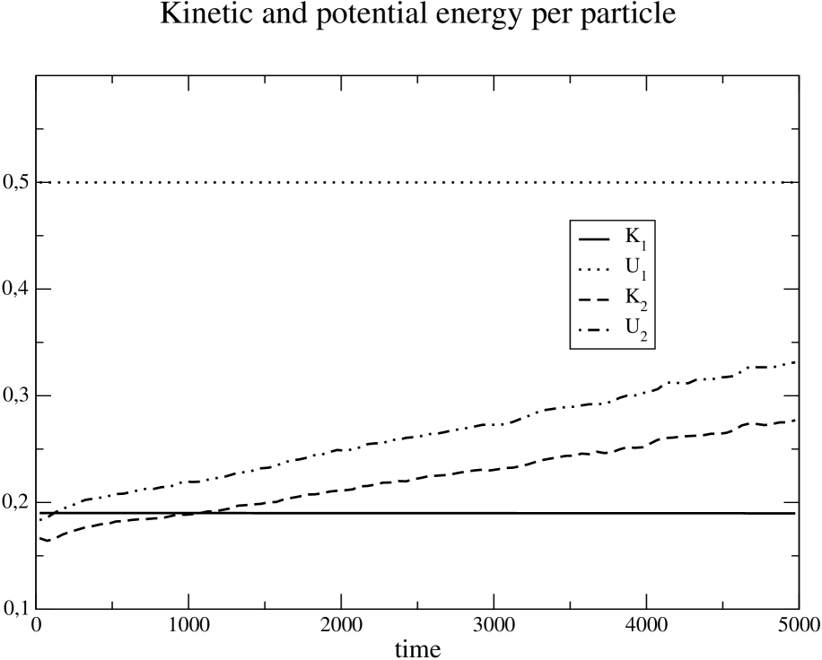
Figure 1: Kinetic and potential energies per particle with $N_{1}=100,000$ (long-range) and $N_{2}=100$ (short-range) obtained from $50$ simulations. The initial energies per particle are $U_{1}=0.69$ and $U_{2}=0.35$, and the time-step used is $\Delta t=0.2$ with an error $\Delta E/E\approx 10^{-8}$. We let both system evolve without coupling until $t=100$ such that system 2 is in a gaussian velocity distribution.

In fact if the long-range interacting system is in contact with a thermal bath at a given temperature, the only possible equilibrium is the Maxwellian distribution. This is essentially the reason why the microcanonical and canonical ensembles are not equivalent. Figure 2a shows the kinetic and potential energies for the case $N_{1}=N_{2}=100,000$. Now the water-bag initial condition is rapidly perturbed when the interaction is turned on and the system evolves to a gaussian velocity distribution, as shown in Figure 2b.

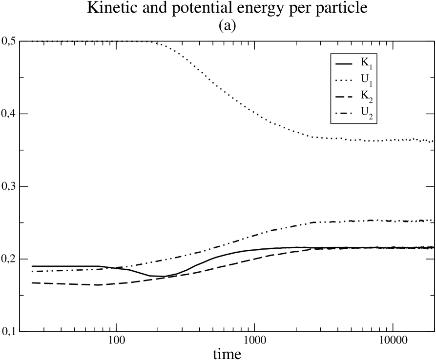
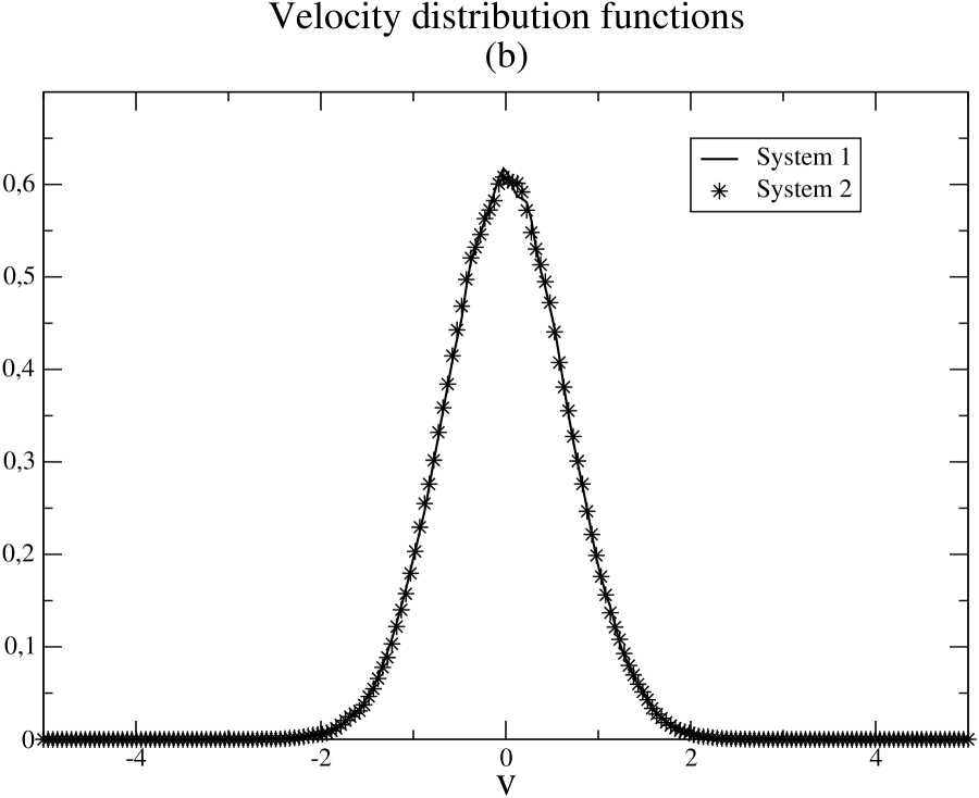
Figure 2: (a) Kinetic and potential energies per particle with $N_{1}=100,000$ and $N_{2}=100,000$ for only one simulation and (b) velocity distribution functions for both systems at $t=20,000$. The interaction is turned on at $t=100$.

We have shown that the condition of maximal entropy subject to the normalization, energy and Casimir constraints is equivalent to the non-linear stability of the stationary states of the Vlasov equation. Therefore, in the mean-field approximation ($N\rightarrow\infty$), the entropy for a system with long-range interaction with a well behaved distribution function depends on an enumerable infinite set of parameters, i. e. the Lagrange multipliers $\lambda_{I}$, $\lambda_{H}$ and $\lambda_{n}$ for $n=2,\ldots,\infty$. These parameters depend in a complicated way on the values of the constraints defined by the initial condition, the latter being difficult to determine in realistic systems. The proposal of the Tsallis statistics, which involves only two free parameters, the temperature and the entropic index $q$, to describe the meta-equilibrium distribution in systems with long-range interaction is therefore limited in scope. It can only describe a specific type of stationary state among an infinity of different possibilities. Even for a finite $N$ system it was shown in Reference r5 that for a water-bag initial condition the system eventually reaches a stationary state with an exponential tail in the distribution, contrary to the power law behavior of the Tsallis statistics. The reasonable fitting of simulation data obtained from the Tsallis functional form stems from the fact that it depends on two parameters, while the Maxwellian depends only on one. Therefore for an even distribution function one can obtain a correct fit up to its fourth moment, while only the dispersion can be fitted correctly using a Maxwellian distribution. It is a well known fact that distribution functions that are well behaved and that have the same first four moments are usually very close. This explains why the Tsallis statistics can give good fitting up to some accuracy. The small differences between the fitted function and the real function can nevertheless be essential as for instance if one needs a correct form for the tails of the distribution. Also the equilibrium properties of such systems are complicated to study since the type of coupling is essential to determine which constraints are kept, while for usual systems only the energy constraint is present and is always preserved.

The Boltzmann-Gibbs entropy is then the correct form to be used. As an importante consequence we note that for a homogeneous state the mean field force vanishes and the entropy is computed using eqs. (3) and $f=\Phi(e({\bf r},{\bf p}))$ with $U=0$, and therefore it is both additive and extensive, even despite the long range-nature of the interaction. For an inhomogeneous state the situation is more complicated and both properties are usually lost. The use of a non-extensive entropy by its own definition is meaningless and may lead to wrong conclusions. The non-extensivity or non-additivity of the entropy results uniquely from the usual definition of the Boltzmann-Gibbs entropy in the presence of correlations among the constituents of the system, as in inhomogeneous states of long-range interacting systems. The use of the Boltzmann-Gibbs entropy is equivalent to suppose that all microstates compatible with the given constraints are equiprobable, which is a quite reasonable assumption. Using any other definition of entropy introduces a non-equiprobability of states, which can result from some “hidden” constraints not considered explicitly (e. g. the Casimir invariants). If this is so, the type of non-equiprobability changes for different values of such constraints, as well as the definition of the entropy, to take account of the change of the probabilities of the microstates. Therefore a fixed form for a generalized entropy cannot take care of all possible types of non-equiprobability.

The authors would like to thank Prof. A. Santana for carefully reading the preliminary version of this paper. This work was partially financed by CNPq (Brazil).

References

- (1) W. Thirring, Z. Phys. 235, 339 (1970).
- (2) D. Lynden-Bell & R. M. Lynden-Bell, MNRAS 181,405 (1977).
- (3) M. Y. Choi & J. Choi, Phys. Rev. Lett. 91, 124101 (2003).
- (4) V. Latora, A. Rapisarda & S. Ruffo, Phys. Rev. Lett. 83, 2104 (1999).
- (5) M. A. Montemurro, F. Tamarit & C. Anteneodo, Phys. Rev. E 67i, 031106 (2003).
- (6) M. Antoni & S. Ruffo, Phys. Rev. E 52i,2361 (1995).
- (7) T. Dauxois, V. Latora, S. Ruffo & A. Torcini, The Hamiltonian Mean Field Model: from Dynamics to Statystical Mechanics and back, in “Dynamics and Thermodynamics of Systems with Long Range Interaction”,T. Dauxois, S. Ruffo, M. wilkens Eds., Lecture Notes in Physics Vol. 602, Springer (2002) - cond-mat/0208456.
- (8) Y. Y. Yamaguchi, J. Barré, F. Bouchet, T. Dauxois & S. Ruffo, Physica A 337i, 36 (2004).
- (9) F. A. Tamarit, G. Maglione, D. A. Stariolo & C. Anteneodo, Phys. Rev. E 71, 036148 (2005).
- (10) A. Campa, A. Giansanti & D. Moroni, Physica A 305, 137 (2002).
- (11) A. Pluchino, V. Latora & A. Rapisarda, Physica D 193, 315 (2004).
- (12) A. Pluchino, V. Latora & A. Rapisarda, Physica A 338, 60 (2005).
- (13) F. Baldovin, L. G. Moyano, A. P. Majtey, A. Robledo & C. Tsallis, Physica A 340, 205 (2004).
- (14) M. Nauenberg, Phys. Rev. E 67, 036114 (2003).
- (15) D. H. Zanette & M. A. Montemurro, Phys. Lett. A 324, 383 (2004).
- (16) W. Braun & K. Hepp, Commun. Math. Phys. 56, 101 (1977).
- (17) P-H. Chavanis, Hamiltonian and Brownian systems with long-range interactions - cond-mat/0409641 (2004).
- (18) L. G. Moyano, F. Baldovin & C. Tsallis, Zeroth principle of thermodynamics in aging quasistationary states - cond-mat/0305091 (2003).
- (19) I. P. Omelyan, I. M. Mryglod & R. Folk, Comp. Phys. Comm. 146, 188 (2002).