Spin relaxation in quantum dots with random spin-orbit coupling

Abstract

We investigate the longitudinal spin relaxation arising due to spin-flip transitions accompanied by phonon emission in quantum dots where the strength of the Rashba spin-orbit coupling is a random function of the lateral (in-plane) coordinate on the spatial nanoscale. In this case the Rashba contribution to the spin-orbit coupling cannot be completely removed by applying a uniform external bias across the quantum dot plane. Due to the remnant random contribution, the spin relaxation rate cannot be decreased by more than two orders of magnitude even when the external bias fully compensates the regular part of the spin-orbit coupling.

I Introduction

A quantum degree of freedom of an electron localized in a quantum dot (QD), i.e. its spin, is thought to be a useful tool for the realization of nanoscale devices that can be used for information processing.Burkard99 ; Elzerman04 The interaction of spins with the environment on the one hand allows necessary read and write procedures on the other hand, leads to losses of the information held by the system. Thus, a critical issue regarding the possibility to convert quantum dots into a hardware realization of quantum information devices is the the ability to manipulate quickly the spins of electrons localized in quantum dots and to keep them in the desired states as long as necessary. The spin-orbit (SO) coupling in QDs plays a crucial role both for the spin manipulation and lifetime of the prepared spin states. For example, the SO coupling allows the effective manipulation of spins by an external electric field due to the fact that the electric field influences the orbital degrees of freedom, and, through the SO coupling, the spin states. The most interesting example of such a manipulation is the electric dipole spin resonance Rashba62 ; Rashba03a , the effect that occurs when the electric field of the incident electromagnetic wave causes spin-flip transitions resonating with the wave frequency. In this case the electric field is a much more efficient tool for manipulating the spins than the magnetic field. The spin states in quantum dots can be prepared and controlled by an external optical field Sham04 too, thus allowing an optical realization of the $write\$and $read$ operations for applications in information technologies.

The SO coupling in two-dimensional systems based on (001)-type structures is described by the sum of the Rashba Rashba84 ; Rashba60 $\hat{H}_{\mathrm{R}}=\alpha_{\mathrm{R}}\left(\sigma_{x}\hat{k}_{y}-\sigma_{y}\hat{k}_{x}\right)$ and Dresselhaus-originatedDyakonov86 $\hat{H}_{\mathrm{D}}^{(001)}=\alpha_{\mathrm{D}}^{(001)}\left(\sigma_{x}\hat{k}_{x}-\sigma_{y}\hat{k}_{y}\right)$ terms, where $\alpha_{\mathrm{R}}$ and $\alpha_{\mathrm{D}}^{(001)}$ are the coupling constants, ${\sigma}$ are the Pauli matrices, and $\mathbf{k}_{\|}=-i\nabla_{\parallel}-(e/c\hbar)\mathbf{A}_{\parallel}$ is the in-plane momentum of electron. Here $e$ is the electron charge, and $\mathbf{A}$ is the vector-potential of the external field. $\hat{H}_{\mathrm{R}}$ and $\hat{H}_{\mathrm{D}}$ terms arise due to the artificial macroscopic asymmetry of the structures and due to the microscopic inversion asymmetry of the unit cells, respectively. For holes the SO Hamiltonian is more sophisticated leading to a more complicated spectra of spin excitations and spin dynamics Rashba88 ; Mauritz99 ; Winkler00 ; Schliemann05 ; Bernevig05 .

In GaAs/Al_xGa_1-xAs structures Stein83 ; Jusserand95 and Si-based transistorsWieck84 , the SO coupling constants typically range from 10^-10 to 10^-9 eV$\cdot$cm. It is important to mention that by applying an external bias across the quantum well, it is possible to manipulate the magnitude of $\alpha$ in InGaAs/InAlAs-based Nitta97 and GaAs/AlAs-based Knap96 ; Miller03 ; Karimov04 systems and even change its sign by doping Koga02 . In the asymmetric Si/Si_1-xGe_x quantum wells investigated in Refs.Jantsch03 ; Tahan05 , where the Dresselhaus term is absent due to the unit cell inversion symmetry and the the band gap is relatively large, the doping-induced SO coupling is three orders of magnitude weaker than in zincblende systems Sarma05 .

The SO coupling not only provides an ability to manipulate spins with an electric field, and thus, hopefully, to design a spin transistor Datta , but also leads to spin relaxation. The Dyakonov-Perel’ mechanismDyakonov72 , which requires random scattering of electrons by impurities and/or phonons, describes the spin relaxation of non-confined electrons in the bulk and in two-dimensional (2D) structures where the electron momentum $k$ is a relatively well defined quantum number. Here the orientation of the spin precession axis in the SO field $\hat{H}_{\mathrm{R}}+\hat{H}_{\mathrm{D}}$ changes randomly through scattering events. The spin ($\gamma_{\mathrm{DP}}$) and momentum relaxation rates are inversely proportional to each other in this case. The resulting spin relaxation rate is $\gamma_{\mathrm{DP}}\sim\alpha^{2}k^{2}\tau$, with $\tau$ being the momentum relaxation time, and $\alpha$ depends on $\alpha_{\mathrm{D}}^{(001)}$ and $\alpha_{\mathrm{R}}$. The spin relaxation can also arise from the random paths of electrons in regular systems of antidots Pershin04 and the tunneling of holes in arrays of Si/Ge QDs Zinovieva05 . Various mechanisms of SO coupling and spin relaxation were reviewed recently in Ref.Zutic04, .

For this reason it is necessary to understand the limits to the abilities to manipulate the electron spins in QDs, where, due to the localization, the electron momentum is not a good quantum number, and thus the spin dynamics Valin02 , and hence the spin relaxation require a more sophisticated consideration. A possible ”admixing” mechanism of spin relaxation in QDs arises since SO coupling mixes the electron states with opposite spins, and, therefore, can cause spin-flip transitions by the emission a phonon Khaetskii00 ; Wu04 ; Florescu04 ; Bastard92 . This effect is a manifestation of an effective spin-phonon coupling caused by the SO interaction. It has been shown, however, that other mechanisms can be important for the spin relaxation. For example, the interaction of the electron spin with the spins of nuclei in GaAs QDs can lead to spin relaxation even if no SO coupling in the Rashba or Dresselhaus form is present Nuclear . This interaction limits the maximal spin relaxation time. In Si-based QDs the spin relaxation can arise due to the modulation of the electron $g-$factor by phonons Kim03 . However, theoretically considered Sherman03a ; Sherman03b ; Golub04 and recently observed Jantsch03 ; Tahan05 Rashba- and Dresselhaus-type SO coupling in 2D Si systems can lead to a more conventional ”admixing” mechanism of the spin relaxation there. We note here that the randomness in SO coupling leads to a Gaussian rather than to an exponential decay of the spin polarization Glazov05 as well as to a serious limitation of the operational modes of the proposed spin transistor devices Sherman05 .

Thus, the possibility to manipulate the spin states depends on the SO coupling strength, which, therefore, plays both a positive and negative role in the spin dynamics of QDs. A solution to this dilemma can be found in the ability to change the strength of the SO coupling by switching it on and off when the desired spin states are produced and preserved, respectively. For example, the effects of the structural asymmetry of a quantum well can be strongly reduced Nitta97 ; Koga02 and/or the Rashba and the Dresselhaus terms can be effectively compensated by applying an external bias Loss02 . If realized experimentally, the suggestion of Ref.Loss02 , is expected to open a route for a larger (up to 100 $\mu$m) size spintronic devices. Sherman05

Here we concentrate on the effect of random SO coupling on spin relaxation in QDs arising in systems where the artificial asymmetry and, in turn, the Rashba-type SO coupling is produced by one-sided doping. The randomness of the SO coupling in our model arises due to fluctuations in the dopant concentration. Because of the randomness, the SO coupling cannot be completely compensated by applying an external bias since the bias is uniform as a function of the in-plane coordinate. We show that even when the bias removes the regular part of the SO coupling, the spin relaxation rate is still finite due to the residual random SO coupling. This effect limits a possible decrease of the spin relaxation rate to two orders of magnitude at most. As another example of the role of inhomogeneous SO coupling in QDs we note its influence on the localization effects Falko03 and on spin dynamics of electrons in quantum rings interacting with the surrounding nuclei Vagner98 .

This paper is organized as follows. Section II presents a model of the random SO coupling in two-dimensional structures and provides us with the basis for the calculations for QDs. In the third Section we present a theory of spin relaxation in QDs with random SO coupling, emphasizing InGaAs-like structures. A summary of the results and a discussion of possible extensions of this work is given in the conclusions.

II Uniform and random SO coupling

In 2D systems where SO coupling arises due to one-sided doping, the $\alpha_{\mathrm{R}}$ parameter cannot be considered as a constant in space since fluctuations of the concentration of the dopant cause its randomness. For doped Si and Ge bulk crystals the importance of randomness of the SO coupling was first understood by Mel’nikov and Rashba Melnikov . Below we consider the dopant fluctuations-induced Rashba field in lateral QDs, calculate the corresponding spin relaxation rate, and show that for applications the randomness imposes important restrictions on the minimum spin-flip rate.

A structure consisting of a 2D channel where the QDs are formed and a narrow dopant layer with a 2D concentration $n(\mathbf{r})$ of dopants with charge $\left|e\right|$ is considered, with $\mathbf{r=(}r_{x},r_{y}\mathbf{)}$ being the 2D in-plane radius-vector. As the factor that determines the local strength of the SO coupling, we consider the $z-$component of the electric field of the dopant ions ${E}_{z}({\bm{\rho}})$ at a point with 2D coordinate ${\bm{\rho}}$ in the well symmetry plane. We assume that the SO coupling is a linear function of ${E}_{z}(\mathbf{\rho})$ with $\alpha_{\mathrm{R}}({\bm{\rho}})=\alpha_{\mathrm{S}O}|e|{E}_{z}({\bm{\rho}})$, where $\alpha_{\mathrm{S}O}$ is a system-dependent parameter that includes the influence of the electric field on the polarization of the electron wavefunction in a quantum well Silva97 ; Grundler99 . The $z$-component of the Coulomb field of the dopant ions is given by

$${E}_{z}({\bm{\rho}})=\frac{\left|{e}\right|}{\epsilon}\int n(\mathbf{r})f({\bm{\rho}},\mathbf{r})d^{2}r,$$ (1)

where $\epsilon$ is the dielectric constant. The integration is performed over the dopant layer. Function $f({\bm{\rho}},\mathbf{r})$ has the form:

$$f({\bm{\rho}},\mathbf{r})=\frac{z_{0}}{[({\bm{\rho}}-\mathbf{r})^{2}+z_{0}^{2}]^{3/2}}.$$ (2)

Here ${\bm{\rho}}=(\rho_{x},\rho_{y})$ is two-dimensional vector characterizing the electron positions in the conducting layer. We assume that the correlation function of the dopant concentration is “white noise” in the form:

$$\langle(n(\mathbf{r}_{1})-\overline{n})(n(\mathbf{r}_{2})-\overline{n})\rangle=\overline{n}\delta(\mathbf{r}_{1}-\mathbf{r}_{2}).$$ (3)

Here $\overline{n}=\langle n(\mathbf{r})\rangle$, and $\left\langle...\right\rangle$ stands for the average. The fluctuations are taken to obey Gaussian statistics, as is commonly considered in the theory of doped semiconductors Efros89 . With the increase of the distance between the layers, the fluctuations of $\alpha_{\mathrm{R}}({\bm{\rho}})$ become smaller and smoother. The total asymmetry-induced Rashba parameter is a sum of a regular average $\langle\alpha\rangle_{a}$ and a random term comprising the zero mean ${\bm{\rho}}$-independent contribution:

$$\alpha_{\mathrm{R}}({\bm{\rho}})=\langle\alpha\rangle_{0}+\alpha_{\mathrm{rnd}}({\bm{\rho}}),$$ (4)

with $\langle\alpha\rangle_{0}=2\pi\alpha_{\mathrm{S}O}\overline{n}e^{2}/\epsilon.$ For the $\delta(z-z_{0})-$doping considered here the magnitude of the random term is given by $\sqrt{\left\langle\alpha_{\mathrm{rnd}}^{2}\right\rangle}=\alpha_{\mathrm{S}O}e^{2}\sqrt{\pi\overline{n}}/\epsilon z_{0}$ Sherman03b . By comparing this result with $\langle\alpha\rangle_{0}$ one concludes that randomness of the SO coupling becomes important when $\sqrt{\langle\alpha_{\mathrm{rnd}}^{2}\rangle}\sim\langle\alpha\rangle_{0},$ that is at $\overline{n}z_{0}^{2}\sim 0.1,$ which is a typical parameter value for zincblende quantum wells Ando ; Winkler . We assume that by applying an external bias $V$ across the QD plane the mean asymmetry-induced term $\langle\alpha\rangle_{a}$ is decreasing as $\langle\alpha\rangle_{a}=\langle\alpha\rangle_{0}\left(V_{c}-V\right)/V_{c}$ and that a critical bias $V_{c}$, which is of the order of few Volts Nitta97 ; Koga02 , fully compensates the mean SO coupling.

The Hamiltonian of the coordinate-dependent SO coupling has to be written in the symmetrized Hermitian form:

$$\hat{H}_{\mathrm{R}}=\frac{1}{2}\left[\sigma_{x}\left\{\hat{k}_{y},\alpha_{\mathrm{R}}\left({\bm{\rho}}\right)\right\}-\sigma_{y}\left\{\hat{k}_{x},\alpha_{\mathrm{R}}\left({\bm{\rho}}\right)\right\}\right],$$ (5)

where $\left\{\hat{k}_{i},\alpha_{\mathrm{R}}\left({\bm{\rho}}\right)\right\}$ stands for the anticommutator.

Quantitatively, the spatial behavior of $\alpha_{\mathrm{R}}({\bm{\rho}})$ is characterized by the correlation function $F_{\mathrm{\alpha\alpha}}\left(\tilde{{\bm{\rho}}}_{12}\right),$ where $\tilde{\bm{\rho}}_{12}\equiv\left({\bm{\rho}}_{1}-{\bm{\rho}}_{2}\right)/z_{0},$ of the random Rashba parameter determined by:

$$\langle\alpha_{\mathrm{R}}({\bm{\rho}}_{1})\alpha_{\mathrm{R}}({\bm{\rho}}_{2}))\rangle=\left\langle\alpha_{\mathrm{rnd}}^{2}\right\rangle F_{\mathrm{\alpha\alpha}}\left(\tilde{{\bm{\rho}}}_{12}\right).$$ (6)

For the Gaussian fluctuations (see, for example Refs. Sherman03a ; Efros89 ), the correlation function in Eq.(6) necessary for describing spin relaxation of semiclassically moving itinerant electrons Sherman03a is:

$$F_{\mathrm{\alpha\alpha}}\left(\tilde{{\bm{\rho}}}_{12}\right)=\frac{2}{\pi}\int\frac{1}{\left[r^{2}+1\right]^{3/2}\left[\left(\mathbf{r-}\tilde{{\bm{\rho}}}_{12}\right)^{2}+1\right]^{3/2}}d^{2}r.$$ (7)

For the following investigations of the spatially random SO coupling in quantum systems Mireles02 described by the Hamiltonian in Eq.(5) we need additional correlation functions of the random Rashba field and its derivatives, namely ($i,j$ are the Cartesian indices $x,y$):

$$\left\langle\alpha_{\mathrm{R}}({\bm{\rho}}_{1})\frac{\partial\alpha_{\mathrm{R}}({\bm{\rho}}_{2})}{\partial\rho_{2}^{(i)}}\right\rangle \equiv \left\langle\alpha_{\mathrm{rnd}}^{2}\right\rangle\frac{F_{\alpha\alpha_{i}}\left(\tilde{{\bm{\rho}}}_{12}\right)}{z_{0}},\qquad$$

$$\left\langle\frac{\partial\alpha_{\mathrm{R}}({\bm{\rho}}_{1})}{\partial\rho_{1}^{(i)}}\alpha_{\mathrm{R}}({\bm{\rho}}_{2})\right\rangle \equiv \left\langle\alpha_{\mathrm{rnd}}^{2}\right\rangle\frac{F_{\alpha_{i}\alpha}\left(\tilde{{\bm{\rho}}}_{12}\right)}{z_{0}},$$

$$\left\langle\frac{\partial\alpha_{\mathrm{R}}({\bm{\rho}}_{1})}{\partial\rho_{1}^{(i)}}\frac{\partial\alpha_{\mathrm{R}}({\bm{\rho}}_{2})}{\partial\rho_{2}^{(j)}}\right\rangle \equiv \left\langle\alpha_{\mathrm{rnd}}^{2}\right\rangle\frac{F_{\alpha_{i}\alpha_{j}}\left(\tilde{{\bm{\rho}}}_{12}\right)}{z_{0}^{2}}.\qquad$$ (8)

The dimensionless correlators can be calculated, for example, as follows:

$$F_{\alpha\alpha_{x}}\left(\tilde{{\bm{\rho}}}_{12}\right) = \frac{6}{\pi}\int\frac{r_{x}}{\left[r^{2}+1\right]^{5/2}\left[\left(\mathbf{r-}\tilde{{\bm{\rho}}}_{12}\right)^{2}+1\right]^{3/2}}d^{2}r,\qquad$$ (9)

$$F_{\alpha_{y}\alpha_{x}}\left(\tilde{{\bm{\rho}}}_{12}\right) = \frac{18}{\pi}\int\frac{r_{y}\left(\mathbf{r-}\tilde{{\bm{\rho}}}_{12}\right)_{x}}{\left[r^{2}+1\right]^{5/2}\left[\left(\mathbf{r-}\tilde{{\bm{\rho}}}_{12}\right)^{2}+1\right]^{5/2}}d^{2}r.$$

Other components of the correlation functions can be obtained from $x\longleftrightarrow y$ permutations. We mention two important properties of the correlators concerning their behavior at small and large distances. The first property is that $F_{\alpha\alpha_{i}}-$type correlators vanish at ${\bm{\rho}}_{1}={\bm{\rho}}_{2}.$ The second property is the fast decay of the long-distance asymptotic of the correlators given, for example, by:

$$F_{\alpha\alpha}\left({\rho}_{12}\gg 1\right) \sim \frac{1}{\tilde{\rho}_{12}^{3}},$$

$$F_{\alpha\alpha_{x}}\left({\rho}_{12}\gg 1\right) \sim \frac{n_{12}^{x}}{\tilde{\rho}_{12}^{4}},$$

$$F_{\alpha_{x}\alpha_{y}}\left({\rho}_{12}\gg 1\right) \sim \frac{n_{12}^{x}n_{12}^{y}}{\tilde{\rho}_{12}^{5}},$$ (10)

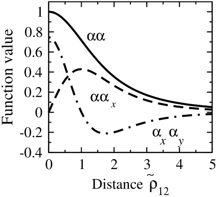
Figure 1: Correlation functions of the random SO coupling parameter $\alpha_{\mathrm{R}}({\bm{\rho}})$ and its derivatives: $F_{\alpha\alpha}$ $(\tilde{{\bm{\rho}}}_{12})$ (solid line), $F_{\alpha\alpha_{x}}$ $(\tilde{{\bm{\rho}}}_{12})$ (dashed line), $F_{\alpha_{x}\alpha_{y}}$ $(\tilde{{\bm{\rho}}}_{12})$ (dash-dotted line); $\tilde{\bm{\rho}}_{12}$ is parallel to the $[110]$ axis.

with the unit vector $\mathbf{n}_{12}=\tilde{{\bm{\rho}}}_{12}/\tilde{\rho}_{12}.$ The correlation functions shown in Fig.1 decay at $\rho_{12}\sim 1,$ and therefore, establish a general spatial nanoscale for the lateral and the $z-$axis directions.

In zincblende-based structures the Dresselhaus SO term arising from the unit cell inversion asymmetry has to be added to the Rashba term. In the (001) structures the coupling parameter $\alpha_{\mathrm{D}}^{(001)}=\alpha_{c}(\pi/w)^{2},$ where $\alpha_{c}$ is the bulk Dresselhaus coupling constant ($\approx 25$ eVA³ in GaAs and InAs [Winkler, ]), and $w$ is the quantum well width. We consider below a model where the random contribution to the Rashba coupling $\left\langle\alpha_{\mathrm{rnd}}^{2}\right\rangle$ is much larger than $\left(\alpha_{\mathrm{D}}^{(001)}\right)^{2},$ which is possible for sufficiently broad quantum wells, and, therefore, neglect the $\hat{H}_{\mathrm{D}}^{(001)}$ term in the calculation procedure and subsequently discuss the role of this term in relation to our results.

Another possibility is provided by (011) QWs, where the Dresselhaus term Dyakonov86 has the form:

$${H}_{D}^{(011)}=\alpha_{D}^{(011)}k_{y}{\sigma}_{z}\left[1-\left(k_{y}^{2}-2k_{x}^{2}\right)w^{2}\pi^{2}\right].$$ (11)

Here the $z-$axis is perpendicular to the QW plane and the in-plane axes are: $x=[100]$ and $y=[0\overline{1}1]$, and $\alpha_{D}^{(011)}=\alpha_{c}(\pi/w)^{2}/2$. The $H_{D}^{(011)}$ coupling proportional to $\sigma_{z}$ does not lead to the electron spin-flip, and, therefore, the main contribution to the spin relaxation rate comes from the randomness.

The strength of the Dresselhaus coupling can be considerably decreased by the strain induced in QWs by a mismatch in the parental lattices, which, therefore, can decrease the contribution of the Dresselhaus terms in the spin relaxation rate in (001) structures.Wu05

III Longitudinal spin relaxation rate

First, we briefly review the influence of the random SO coupling on the spin relaxation of non-confined electrons in quantum wells. The spin precession rate and direction at a point ${\bm{\rho}}$ are determined by the random local coupling $\alpha_{\mathrm{R}}\left({\bm{\rho}}\right)$. As a result, the spin precession is random even for a carrier moving straightforwardly and the total spin of the electron ensemble relaxes even if the regular term $\langle\alpha\rangle_{a}$ vanishes as a result of applying either an external bias or equivalent doping at the other side of the conducting layer Sherman03a .

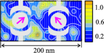
Figure 2: (Color online) Two quantum dots on a template with a random Rashba SO coupling. The arrows show schematically the spin orientations. The gates form the confining in-plane potential. The scale on the right represents the Rashba parameter in 10^-9 eVcm units, $\langle\alpha\rangle=0.5\times 10^{-9}$ eVcm, $\overline{n}=2.5\times 10^{11}$ cm^-2, and $z_{0}=10$ nm.

Now we consider a single-electron QD produced by applying a lateral bias to a 2D electron gas (see Fig. 2) leading to electron localization. From the experimental point of view, we shall concentrate on In_0.5Ga_0.5As$-$like systems, where the ability to manipulate the SO coupling by a moderate bias applied across the structure has been clearly proven Nitta97 ; Koga02 .

The spectrum of an electron in the QD, $E_{n,\ell_{z}},$ is determined both by the confinement potential $m^{*}\rho^{2}\omega^{2}/2$ (Fig. 2 shows two quantum dots on the random Rashba SO coupling background) and the uniform static magnetic field $\mathbf{B}\parallel z$ with the axial gauge $\mathbf{A}=[\mathbf{B},\mathbf{r]}/2$, respectively, leading to

$$E_{n,\ell_{z}}=-\ell_{z}\frac{\hbar^{2}}{2m^{*}l_{B}^{2}}+\frac{\hbar^{2}}{2m^{*}a^{2}}\left(1+\left|\ell_{z}\right|+2n\right)\pm\frac{g\mu_{B}}{2}B,$$ (12)

where $m^{*}$ is the lateral electron effective mass, $\ell_{z}$ is the $z-$component of the orbital momentum, $n$ is the radial quantum number, and the corresponding wave function

$$\psi_{n\ell_{z}}({\bm{\rho}})\left|s\right\rangle=\frac{1}{\sqrt{2\pi}a}\exp(-\rho^{2}/4a^{2})L_{n\ell_{z}}(\rho/a)e^{i\ell_{z}\varphi}\left|s\right\rangle.$$ (13)

Here $\varphi$ is the azimuthal angle, the magnetic length $l_{B}=\sqrt{\hbar c/\left|e\right|B}$, $L_{n\ell_{z}}(\rho/a)$ is a Laguerre polynomial, and the spatial scale $a=l_{0}l_{B}\left(l_{0}^{4}+l_{B}^{4}\right)^{-1/4},$ with $l_{0}=\sqrt{\hbar/2m^{*}\omega}$ being the ”oscillator” length in the absence of a magnetic field due to the lateral confinement forming the QD, $\hbar\omega$ is the separation of the energy levels at $B=0$, and $\left|s\right\rangle=\left|\uparrow\right\rangle$,$\left|\downarrow\right\rangle$ is the spin state. With the increase of magnetic field, $E_{n,\ell_{z}}$ changes from the spectrum of a single-electron QD to the spectrum of a free electron in a magnetic field.

We consider below the QD in only the orbital ground state with the function

$$\psi_{00}({\bm{\rho}})=\frac{1}{\sqrt{2\pi}a}\exp(-\rho^{2}/4a^{2}).\qquad$$ (14)

The spin-flip-transitions such as $\psi_{00}({\bm{\rho}})\left|\uparrow\right\rangle\rightarrow\psi_{00}({\bm{\rho}})\left|\downarrow\right\rangle$ without change of the orbital quantum numbers occur at a frequency $\omega=\left|g\right|\mu_{B}B/\hbar$ and the transition energy is released to an acoustic phonon with momentum $q=\left|g\right|\mu_{B}B/c_{\lambda}\hbar,$ where $c_{\lambda}$ is the sound velocity for the given phonon branch $\lambda$ with $\lambda=\parallel$ and $\lambda=\perp$ for the longitudinal and the transverse modes, respectively. The electron-phonon coupling Hamiltonian for acoustic phonons $\hat{H}_{\mathrm{e-ph}}$ has the form

$$\hat{H}_{\mathrm{e-ph}}=\sum_{\lambda}\left(\hat{H}_{\mathrm{e-ph,}P}^{[\lambda]}+\hat{H}_{\mathrm{e-ph,}D}^{[\lambda]}\right),$$

arising due to the piezoeffect $\left(\hat{H}_{\mathrm{e-ph,}P}^{[\lambda]}\right)$ and due to the deformation potential $\left(\hat{H}_{\mathrm{e-ph,}D}\right).$ These terms have the form (assuming the crystal volume equal to one):

$$\hat{H}_{\mathrm{e-ph},P}^{[\lambda]} = \sqrt{2\pi}\frac{\kappa_{14}}{\sqrt{\zeta}}\frac{e}{\epsilon}\sum_{\mathbf{q,e}}\frac{1}{\sqrt{qc_{\lambda}}}\left[e_{x}e_{y}d^{z}+e_{z}e_{x}d^{y}+e_{y}e_{z}d^{x}\right]\left(e^{-i\mathbf{qr}}\hat{b}_{\lambda,\mathbf{q,e}}^{\dagger}+\mathrm{h.c}\right),$$

$$\hat{H}_{\mathrm{e-ph,}D}^{[\lambda]} = \frac{D\sqrt{\hbar}}{\sqrt{2\zeta c_{\lambda}}}\sum_{\mathbf{q,e}}\sqrt{q}\left(\mathbf{de}\right)\left(e^{-i\mathbf{qr}}\hat{b}_{\lambda,\mathbf{q,e}}^{\dagger}+\mathrm{h.c}\right),$$ (15)

where the summation is taken over the phonon momenta $\mathbf{q}$, and polarization $\mathbf{e}.$ The propagation direction $\mathbf{d=q}/q$, $\kappa_{14}$ is the strength of the piezointeraction, $D$ is the deformation potential, $\zeta$ is the crystal density, $\epsilon$ is the dielectric constant, and $\hat{b}_{\lambda,\mathbf{q,e}}^{\dagger}$ is the phonon creation operator. $\hat{H}_{\mathrm{e-ph,}D}^{[\lambda]}$ is nonzero for the longitudinal phonon mode ($\mathbf{de}=1$) only. At finite temperature, the application of Fermi’s golden rule yields the mean value of the spin relaxation rate $\left\langle\Gamma_{1}\right\rangle\equiv\left\langle T_{1}^{-1}\right\rangle$, where $T_{1}$ is the relaxation time, with respect to the spin-flip as:

$$\left\langle\Gamma_{1}\right\rangle=\frac{2\pi}{\hbar}\left[n_{B}+1\right]\sum_{\lambda}\nu_{\mathrm{ph}}^{[\lambda]}\left(\left|g\right|\mu_{B}B\right)\left\langle\left|\left\langle\tilde{s}^{\prime}\right|\tilde{\psi}_{\mathrm{gr}}({\bm{\rho}})\left|\hat{H}_{\mathrm{e-ph}}^{[\lambda]}\right|\tilde{\psi}_{\mathrm{gr}}(\mathbf{\rho})\left|\tilde{s}\right\rangle\right|^{2}\right\rangle_{\mathbf{d,e}},$$ (16)

where $n_{B}=$ $\left[\exp\left(\left|g\right|\mu_{B}B/T\right)-1\right]^{-1}$ is the Bose-Einstein phonon occupation factor. We consider below only the zero temperature case for simplicity. The phonon density of states $\nu_{\mathrm{ph}}^{[\lambda]}\left(\varepsilon\right)$ $=\varepsilon^{2}/2\pi^{2}(\hbar c_{\lambda})^{3},$ and $\left\langle...\right\rangle_{\mathbf{d,e}}$ stands for the average over the phonon directions and polarizations. The spin-flip matrix element of $\hat{H}_{\mathrm{e-ph}}$ is nonzero due to the admixing of the upper $\psi_{n\ell_{z}}({\bm{\rho}})\left|s\right\rangle$ states to the ground state $\tilde{\psi}_{\mathrm{gr}}{\bm{\rho}})\left|\tilde{s}\right\rangle,$ where $\left|\tilde{s}\right\rangle$ shows that spin is an approximate quantum number due to the SO coupling. Here we have neglected the spin splitting of the states $g\mu_{B}B$ in comparison to the energy corresponding to the orbital degrees of freedom, $\hbar\omega_{n\ell_{z}}$. The approximation is a reasonable one despite the large $g-$factor in In_0.5Ga_0.5As ($g\approx 4.0$) quantum wells, since a small effective mass $\left(m^{*}=0.04m_{0}\right)$ leads to $g\mu_{B}B/\hbar\omega_{n\ell_{z}}\leq 0.2$. We mention here that due to the random coordinate dependence of the Hamiltonian $\hat{H}_{\mathrm{R}}$, there are no symmetry-related selection rules for $n$ and $\ell_{z}$ in the matrix elements $\left\langle s^{\prime}\right|\psi_{n\ell_{z}}({\bm{\rho}})\left|\hat{H}_{\mathrm{R}}\right|\psi_{00}({\bm{\rho}})\left|s\right\rangle$ that are responsible for the formation of the spin relaxation rate, in contrast to the case of regular SO coupling Wu04 . Since the Hamiltonians $\hat{H}_{\mathrm{e-ph}}^{[\lambda]}$ and $\hat{H}_{\mathrm{e-ph,}D}^{[\lambda]}$ have drastically different phonon momentum dependencies, the relative contribution of the deformation potential mechanism increases with an increase in the magnetic field Alcalde04 . Due to the large $g$-factor, this mechanism already dominates at $B=0.1$ T.

By using the approach suggested in Ref.Khaetskii00 and taking into account the Gaussian character of the fluctuations, after some algebraic transformations we obtain for the deformation potential contribution using the notation $\mathbf{0}\equiv\left(0,0\right),\mathbf{1}\equiv\left(n_{1},\ell_{1}^{z}\right),\mathbf{2}\equiv\left(n_{2},\ell_{2}^{z}\right):$

$$\left\langle\Gamma_{1}\right\rangle = \frac{\left(g\mu_{B}\right)^{5}}{4\hbar^{4}}\frac{D^{2}}{\zeta c_{\parallel}^{5}}B^{5}\sum_{\mathbf{1,2}}\frac{1}{\omega_{n_{1},\ell_{1}^{z}}^{2}\omega_{n_{2},\ell_{2}^{z}}^{2}}\times$$

$$\left[\left\langle K_{-}(\mathbf{1})K_{-}^{*}(\mathbf{2})\right\rangle\left\langle g_{\parallel}(\mathbf{0};\mathbf{1})g_{\parallel}^{*}(\mathbf{0};\mathbf{2})\right\rangle_{\mathbf{d}}+\left\langle K_{-}(\mathbf{1})K_{+}^{*}(\mathbf{2})\right\rangle\left\langle g_{\parallel}(\mathbf{0};\mathbf{1})g_{\parallel}^{*}(\mathbf{2};\mathbf{0})\right\rangle_{\mathbf{d}}\right.+$$

$$\left.\left\langle K_{+}(\mathbf{1})K_{-}^{*}(\mathbf{2})\right\rangle\left\langle g_{\parallel}(\mathbf{1};\mathbf{0})g_{\parallel}^{*}(\mathbf{0};\mathbf{2})\right\rangle_{\mathbf{d}}+\left\langle K_{+}(\mathbf{1})K_{+}^{*}(\mathbf{2})\right\rangle\left\langle g_{\parallel}(\mathbf{1};\mathbf{0})g_{\parallel}^{*}(\mathbf{2};\mathbf{0})\right\rangle_{\mathbf{d}}\right].$$

The correlators are given by :

$$\left\langle K_{-}(\mathbf{1})K_{-}^{*}(\mathbf{2})\right\rangle = K_{yy}+K_{xx}-iK_{xy}+iK_{yx},$$

$$\left\langle K_{+}(\mathbf{1})K_{+}^{*}(\mathbf{2})\right\rangle = K_{yy}+K_{xx}+iK_{xy}-iK_{yx},$$

$$\left\langle K_{-}(\mathbf{1})K_{+}^{*}(\mathbf{2})\right\rangle = K_{yy}-K_{xx}-iK_{xy}-iK_{yx},$$

$$\left\langle K_{+}(\mathbf{1})K_{-}^{*}(\mathbf{2})\right\rangle = K_{yy}-K_{xx}+iK_{xy}+iK_{yx},$$

with the matrix elements averaged over the disorder:

$$K_{ji} = \left\langle\alpha_{\mathrm{rnd}}^{2}\right\rangle\int\psi_{n_{2}\ell_{2}^{z}}({\bm{\rho}}_{2})\psi_{n_{1}\ell_{1}^{z}}({\bm{\rho}}_{1})\times$$ (18)

$$\left\{F_{\alpha\alpha}({\bm{\rho}}_{12})\hat{\overline{P}}_{j}^{(2)}\hat{P}_{i}^{(1)}+\frac{i}{z_{0}}\left(F_{\alpha_{j}\alpha}({\bm{\rho}}_{12})\hat{P}_{i}^{(1)}-F_{\alpha\alpha_{i}}({\bm{\rho}}_{12})\hat{\overline{P}}_{j}^{(1)}\right)+\frac{F_{\alpha_{j}\alpha_{i}}({\bm{\rho}}_{12})}{z_{0}^{2}}\right\}\cdot$$

$$\psi_{00}({\bm{\rho}}_{2})\psi_{00}({\bm{\rho}}_{1})d^{2}\rho_{1}d^{2}\rho_{2}+$$

$$\left\langle\alpha\right\rangle_{a}^{2}\int\psi_{n_{2}\ell_{2}^{z}}({\bm{\rho}}_{2})\psi_{n_{1}\ell_{1}^{z}}({\bm{\rho}}_{1})\hat{\overline{P}}_{j}^{(2)}\hat{P}_{i}^{(1)}\psi_{00}({\bm{\rho}}_{2})\psi_{00}({\bm{\rho}}_{1})d^{2}\rho_{1}d^{2}\rho_{2}.$$

The operators $\hat{P}_{i}^{(1)},\hat{P}_{j}^{(2)}$ in Eq.(18) are defined according to

$$P_{x}^{(1)}=-\frac{\rho_{1y}}{l_{B}^{2}}-2i\frac{\partial}{\partial\rho_{1x}},\qquad P_{y}^{(1)}=\frac{\rho_{1x}}{l_{B}^{2}}-2i\frac{\partial}{\partial\rho_{1y}},$$ (19)

and act on the wavefunction $\psi_{00}({\bm{\rho}}_{1})$ and $\psi_{00}({\bm{\rho}}_{2})$, respectively.

The matrix elements $g_{\lambda}(n,\ell_{z};\mathbf{0})$ of the phonon emission due to electron-phonon coupling are

$$g_{\lambda}(n,\ell_{z};\mathbf{0})=\int\psi_{0}^{2}(z)\psi_{n,\ell_{z}}^{*}({\bm{\rho}})e^{i\mathbf{q}_{\lambda}\mathbf{r}}\psi_{00}({\bm{\rho}})d^{3}r.$$ (20)

where $\psi_{0}(z)$ corresponds to the $z-$axis quantization and is assumed here for simplicity to be the rigid-walls wave function $\psi_{0}(z)=\sqrt{2/w}\sin(\pi z/w)$. Since we consider broad quantum wells, where the size quantization energy is relatively small and the electron wavefunction weakly penetrates into the interfaces, the rigid-walls boundary conditions are justified.

We now consider two applications of the model described above. First, we consider the effect of the fully compensated Rashba coupling ($V=V_{c}$) such that we are left only with the random contribution $\alpha_{\mathrm{rnd}}({\bm{\rho}})$ with $\left\langle\alpha_{\mathrm{rnd}}({\bm{\rho}})\right\rangle=0$. Fig. 3 presents the results of numerical calculations (including a small contribution of the piezoeffect interaction) of the spin relaxation rate for In_0.5Ga_0.5As quantum dots as a function of the magnetic field $B$ using Eqs.(12)-(18) assuming $D=7.5$ eV (Ref.[Dpot, ]), $\kappa_{14}=-0.1$ Cm^-2 (Ref.[Gantmakher87, ]), and sound velocities $c_{\parallel}=4.7\cdot 10^{5}$ cm/s and $c_{\perp}=2.8\cdot 10^{5}$ cm/s for the longitudinal and transverse phonons, respectively (Ref. [Gantmakher87, ]). As can be seen, the spin-flip rate increases very rapidly with the applied field, analogous to the case of regular SO coupling Khaetskii00 ; Alcalde04 .

Second, we investigate the bias dependence of the spin relaxation rate $\left\langle\Gamma_{1}\left(V\right)\right\rangle$ corresponding to the linear dependence of the mean Rashba parameter $\langle\alpha\rangle_{a}$ on the applied bias. In this case, it follows from Eq.(18), that this dependence can be presented in the form:

$$\frac{\left\langle\Gamma_{1}(0)\right\rangle}{\left\langle\Gamma_{1}\left(V\right)\right\rangle}=$$

$$\frac{\left\langle\Gamma_{1}(0)\right\rangle}{\left\langle\Gamma_{1}\left(V_{c}\right)\right\rangle+\left[\left\langle\Gamma_{1}(0)\right\rangle-\left\langle\Gamma_{1}\left(V_{c}\right)\right\rangle\right]\left(\left(V_{c}-V\right)/V_{c}\right)^{2}}.$$ (21)

Figure 4 shows the $\left\langle\Gamma_{1}(0)\right\rangle/\left\langle\Gamma_{1}\left(V\right)\right\rangle$ ratio for the two structures presented in Fig.3. As can be seen in Fig.4, the resulting $\left\langle\Gamma_{1}(V_{c})\right\rangle$, (when there is full compensation $\left(\langle\alpha\rangle_{a}=0\right),$) for $z_{0}=10$ nm is approximately 60 times smaller than $\left\langle\Gamma_{1}(0)\right\rangle$. The residual relaxation rate decreases rapidly with the increase of the dopant-plane layer distance, corresponding to a decrease in the random fluctuations of the SO coupling.

We note that the randomness of $\alpha_{\mathrm{rnd}}({\bm{\rho}})$ leads to an inhomogeneous broadening $\sigma_{\Gamma}=\left\langle\left(\Gamma_{1}-\left\langle\Gamma_{1}\right\rangle\right)^{2}\right\rangle^{1/2}$ of the spin-flip transitions making the relaxation rate dependent on the QD position. For the Gaussian fluctuations the broadening $\sigma_{\Gamma}$ becomes of the order of the mean value of $\Gamma_{1}$ at full compensation ($V=V_{c}$). The effect of inhomogeneous broadening can be seen clearly when the lateral confinement of the wave function $a$ is considerably smaller than the spatial scale of the fluctuations of the random potential $z_{0}.$ In this case each QD in the ensemble interacts mostly with the local Rashba field $\alpha({\bm{\rho}}_{0})$, where ${\bm{\rho}}_{0}$ is the position of the QD, that in this case varies weakly on the spatial scale of $a.$ In the case of full compensation, the relaxation rate for each QD is proportional to the local $\alpha_{\mathrm{rnd}}^{2}({\bm{\rho}}_{0})$ leading to an inhomogeneous width of the transition of the order of $\left\langle\alpha_{\mathrm{rnd}}^{2}\right\rangle,$ being, therefore, of the order of $\left\langle\Gamma_{1}\right\rangle$ itself. Experimentally, this situation can be realized, for example, in strong magnetic fields $B>10$ T, where the magnetic length $l_{B}<10$ nm. In the $a\ll z_{0}$ limit the ratio of the relaxation rates, which can be found from the discussion following Eq.(4), becomes $\left\langle\Gamma_{1}(V_{c})\right\rangle/\left\langle\Gamma_{1}\left(0\right)\right\rangle=\left\langle\alpha_{\mathrm{rnd}}^{2}\right\rangle/\left\langle\alpha\right\rangle_{0}^{2}=1/8\pi\overline{n}z_{0}^{2}.$

We now discuss the relative role of the random Rashba and Dresselhaus SO interactions since both effects contribute to the relaxation rate at $V=V_{c}.$ In an In_0.5Ga_0.5As quantum dot of the width $w=$15 nm, as presented in Figs. 3 and 4, the Dresselhaus term $\alpha_{D}^{(001)}$ is of approximately $1.25\times 10^{-10}$ eVcm. At the same time, the one-side doping with $\overline{n}=8\times 10^{11}$ cm^-2 leads to $\left\langle\alpha\right\rangle_{0}\approx 10^{-9}$ eVcm, giving in this case $\left\langle\Gamma_{1}(0)\right\rangle/\left\langle\Gamma_{1}\left(V_{c}\right)\right\rangle\sim 60.$ Therefore, the Dresselhaus and the random Rashba terms give similar contributions to the spin relaxation under these conditions. The ratio of these contributions depends on the applied magnetic field, and numerical analysis shows that the random part can dominate over the regular one. For (011) structures the random part gives the major contribution.

IV Conclusions

In this analysis we have found that due to fluctuations of the SO coupling, the spin relaxation in QDs does not vanish even in the case of full compensation of the mean value of the SO coupling by an external bias. The residual spin relaxation rate is of the order of few percent of the spin relaxation rate in the case of a non-compensated field and strongly depends on the system properties, the size of the dot, and the applied magnetic field. In the case of full compensation, the inhomogeneous line width of the spin-flip transition is of the order of the mean line frequency, and, therefore, one has a broad distribution of the relaxation rates over the ensemble of QDs. The effect of the random Rashba SO coupling is comparable to or larger than the effect of the Dresselhaus coupling. The ratio of the contributions of these SO coupling mechanisms to the spin relaxation rate is compound- and structure-dependent, and shows that the importance of the randomness of the Rashba SO coupling.

We concentrated here on the longitudinal spin relaxation time $T_{1}=\Gamma_{1}^{-1}$ that is related to the energy release to the acoustic phonon bath in the spin-flip process. However, the spin ensemble dephasing time $T_{2},$ describing the motion of the spin component perpendicular to the magnetic field, and which may not be related to the energy transfer from the spin system to the lattice, is an important characteristic of a QD ensemble. As was recently found theoretically, the physics behind these two relaxation processes in systems of QDs coupled to phonons is similar Golovach04 . Therefore, the randomness of the SO coupling considered above also influences the dephasing time $T_{2}$. This is an interesting problem which will be investigated separately. The role of the magnetic field parallel to the plane Falko05 of the QD would be another extension of the results presented here.

In this paper we have discussed zincblende quantum dots only. However, some remarks concerning Si-based structures need to be given. If the admixing mechanism of spin relaxation in these structures becomes important, the arguments discussed above concerning the role of the randomness could be applied there to an even larger extent due to the absence of the Dresselhaus term. A quantitative analysis of this problem necessitates a comparison of the effectiveness of different mechanisms of spin relaxation in Si-based QDs, which is a separate interesting issue.

V Acknowledgment

This work was supported by the DARPA SpinS program and the Austrian Science Fund FWF via grant P15520. EYS is grateful to J.E. Sipe for very valuable discussions.

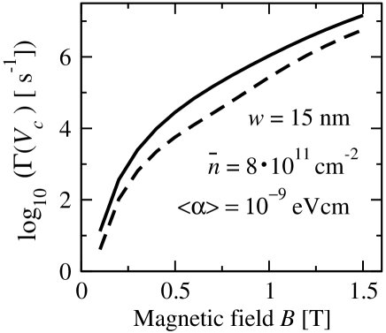
Figure 3: Logarithm of the spin relaxation rate as a function of applied magnetic field for different $z_{0}$ in the case of total compensation of the regular SO coupling by an external bias ($V=V_{c}$); $z_{0}=10$ nm (solid line), $z_{0}=20$ nm (dashed line), and $l_{0}=15$ nm. The relationship between the doping $\overline{n}$ and Rashba constant $\langle\alpha\rangle$ corresponds to the experimental data of Ref. [Koga02, ].

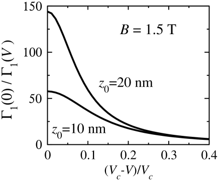
Figure 4: The ratio of longitudinal spin relaxation rates $\left\langle\Gamma_{1}(0)\right\rangle/\left\langle\Gamma_{1}(V)\right\rangle$ as a function of the applied bias that is gradually compensating the SO coupling. The applied magnetic field $B=1.5$ T.

References

- (1) G. Burkard, D. Loss, and D.P. DiVincenzo, Phys. Rev. B 59, 2070 (1999)
- (2) J. M. Elzerman, R. Hanson, L. H. W. van Beveren, B. Witkamp, L. M. K. Vandersypen, L. P. Kouwenhoven, Nature 430, 431 (2004)
- (3) E.I. Rashba and V.I. Sheka, Sov. Phys. - Solid State 3, 1718 (1962) (Fizika Tverdogo. Tela 3, 2369 (1961))
- (4) E.I. Rashba and Al. L. Efros, Phys. Rev. Lett. 91, 126405 (2003), E. I. Rashba and Al. L. Efros, Appl. Phys. Lett. 83, 5295 (2003)
- (5) P. Chen, C. Piermarocchi, L. J. Sham, D. Gammon, and D. G. Steel, Phys. Rev. B 69, 075320 (2004)
- (6) Yu. A. Bychkov and E. I. Rashba, JETP Lett. 39, 79 (1984), E.I. Rashba, Sov. Phys. - Solid State 2, 1874, (1964)
- (7) E.I. Rashba, Sov. Phys. - Solid State 2, 1109 (1960) (Fizika Tverdogo Tela 2, 1224 (1960))
- (8) M.I. Dyakonov and V.Yu. Kachorovskii, Sov. Phys. Semicond. 20, 110 (1986)
- (9) E.I. Rashba and E.Ya. Sherman, Phys. Lett. A 129, 175 (1988)
- (10) O. Mauritz and U. Ekenberg, Phys. Rev. B 60, R8505 (1999)
- (11) R. Winkler, S.J. Papadakis, E.P. De Poortere, and M. Shayegan, Phys. Rev. Lett. 85, 4574 (2000)
- (12) J. Schliemann and D. Loss, Phys. Rev. B 71, 085308 (2005)
- (13) B. A. Bernevig and S.-C. Zhang Phys. Rev. Lett. 95, 016801 (2005)
- (14) D. Stein, K. v. Klitzing, and G. Wiemann, Phys. Rev. Lett. 51, 130 (1983)
- (15) B. Jusserand, D. Richards, G. Allan, C. Priester, and B. Etienne, Phys. Rev. B 51, 4707 (1995)
- (16) A. D. Wieck, E. Batke, D. Heitmann, J. P. Kotthaus, and E. Bangert, Phys. Rev. Lett. 53, 493 (1984)
- (17) J. Nitta, T. Akazaki, H. Takayanagi, and T. Enoki, Phys. Rev. Lett. 78, 1335 (1997)
- (18) W. Knap, C. Skierbiszewski, A. Zduniak, E. Litwin-Staszewska, D. Bertho, F. Kobbi, and J. L. Robert, G. E. Pikus, F. G. Pikus, S. V. Iordanskii, V. Mosser, K. Zekentes, Yu. B. Lyanda-Geller, Phys. Rev. B 53, 3912 (1996)
- (19) J. B. Miller, D. M. Zumbühl, C. M. Marcus, Y. B. Lyanda-Geller, D. Goldhaber-Gordon, K. Campman, and A. C. Gossard, Phys. Rev. Lett. 90, 076807 (2003)
- (20) O. Z. Karimov, G. H. John, R. T. Harley, W. H. Lau, M. E. Flatté, M. Henini, and R. Airey, Phys. Rev. Lett. 91, 246601 (2003)
- (21) T. Koga, J. Nitta, T. Akazaki, and H. Takayanagi, Phys. Rev. Lett. 89, 046801 (2002)
- (22) Z. Wilamowski, W. Jantsch, N. Sandersfeld, M. Mühlberger, F. Schäffler, and S. Lyon, Physica E 6, 111 (2003); Z. Wilamowski, W. Jantsch, H. Malissa, and U. Rößler, Phys. Phys. Rev. B 66, 195315 (2002).
- (23) C. Tahan and R. Joynt, Phys. Rev. B 71, 075315 (2005)
- (24) For theory of Si-based spintronics see: S. Das Sarma, R. de Sousa, X. Hu and B. Koiller, Solid State Communications 133, 737 (2005); K.S. Virk and J.E. Sipe, cond/mat 0502629 (unpublished).
- (25) S. Datta and B. Das, Appl. Phys. Lett. 56, 665 (1990)
- (26) M.I. Dyakonov and V.I. Perel’, Sov. Phys. -Solid State 13, 3023 (1972)
- (27) Y. V. Pershin and V. Privman, Phys. Rev. B 69, 073310 (2004)
- (28) A. F. Zinovieva, A. V. Nenashev, and A. V. Dvurechenskii, Phys. Rev. B 71, 033310 (2005)
- (29) I. Zutic, J. Fabian and S. Das Sarma, Rev. Mod. Phys. 76, 323 (2004)
- (30) M. Valin-Rodriguez, A. Puente, L. Serra, and E. Lipparini, Phys. Rev. B 66, 235322 (2002)
- (31) A. V. Khaetskii and Y. V. Nazarov, Phys. Rev. B 61, 12639 (2000), and Phys. Rev. B 64, 125316 (2001)
- (32) J.L. Cheng, M.W. Wu, and C. Lu, Phys. Rev. B 69, 115318 (2004)
- (33) For two-electron systems see: M. Florescu, S. Dickman, M. Ciorga, A. Sachrajda, and P. Hawrylak, Physica E 22, 414 (2004).
- (34) G. Bastard, Phys. Rev. B46, 4253 (1992) and D. M. Frenkel, ibid, 43, 14228 (1991) discussed spin relaxation in QWs in a strong magnetic field. For non-quantizing fields see: E. L. Ivchenko, Fiz. Tverd. Tela (Leningrad) 15, 1566 (1973), [Sov. Phys. Solid State 15, 1048 (1973)]; M. M. Glazov, Phys. Rev. B 70, 195314 (2004).
- (35) S. I. Erlingsson, Y. V. Nazarov, and V. I. Fal’ko, Phys. Rev. B 64, 195306 (2001); A. Khaetskii, D. Loss, and L. Glazman, Phys. Rev. B 67, 195329 (2003); I. Tifrea and M. E. Flatté, Phys. Rev. B 69, 115305 (2004)
- (36) B.A. Glavin and K.W. Kim, Phys. Rev. B 68, 045308 (2003), Y.G. Semenov and K.W. Kim, Phys. Rev. Lett. 92, 026601 (2004)
- (37) E.Ya. Sherman, Appl. Phys. Lett. 82, 209 (2003)
- (38) E.Ya. Sherman, Phys. Rev. B 67, R 161303 (2003)
- (39) L. E. Golub and E. L. Ivchenko, Phys. Rev. B 69, 115333 (2004)
- (40) M.M. Glazov and E.Ya. Sherman, Phys. Rev. B 71, 241312 (2005)
- (41) E.Ya. Sherman and J. Sinova, Phys. Rev. B 72, 075318 (2005)
- (42) J. Schliemann, J. C. Egues, and D. Loss, Phys. Rev. Lett. 90, 146801 (2003)
- (43) J.-H. Cremers, P. W. Brouwer, and V. I. Fal’ko, Phys. Rev. B 68, 125329 (2003)
- (44) I. D. Vagner, A. S. Rozhavsky, P. Wyder, and A. Yu. Zyuzin, Phys. Rev. Lett. 80, 2417 (1998).
- (45) V.I. Mel’nikov and E.I. Rashba, Sov. Phys. JETP 34, 1353 (1972)
- (46) A.L. Efros and B.I. Shklovskii, Electronic Properties of Doped Semiconductors, Springer, Heidelberg (1989)
- (47) For a quantum approach to spintronics, see: F. Mireles and G. Kirczenow, Europhys. Lett. 59, 107 (2002)
- (48) For the kp-calculations of see: E.A.A. Silva, G.C. La Rocca, and F. Bassani, Phys. Rev. B 55, 16293 (1997)
- (49) D. Grundler, Phys. Rev. Lett. 84, 6074 (2000)
- (50) T. Ando, A.B. Fowler, and F. Stern, Rev. Mod. Phys. 54, 437 (1982)
- (51) R. Winkler, Spin-orbit Coupling Effects in Two-Dimensional Electron and Hole Systems (Springer Tracts in Modern Physics, 2003)
- (52) L. Jiang and M. W. Wu, Phys. Rev. B 72, 033311 (2005)
- (53) A. M. Alcalde, Q. Fanyao and G. E. Marques, Physica E 20, 228 (2004)
- (54) For calculations and experimental data of the deformation potential in GaAs and InAs see: C. Priester, G. Allan, and M. Lannoo Phys. Rev. B 37, 8519 (R) (1988); M. Cardona and N. E. Christensen, Phys. Rev. B 35, 6182 (1987); Landolt-Bornstein: Numerical Data and Functional Relationships in Science and Technology, edited by O. Madelung (Spinger-Verlag, Berlin, 1982)
- (55) V.F. Gantmakher and Y.B. Levinson, Carrier Scattering in Metals and Semiconductors (North-Holland, Amsterdam, 1987).
- (56) V. N. Golovach, A. Khaetskii, and D. Loss, Phys. Rev. Lett. 93, 016601 (2004)
- (57) V.I. Fal’ko, B.L. Altshuler, and O. Tsyplyatyev, Phys. Rev. Lett. 95, 076603 (2005)