Spin polarization of edge states and magnetosubband structure in quantum wires

Abstract

We provide a quantitative description of the structure of edge states in split-gate quantum wires in the integer quantum Hall regime. We develop an effective numerical approach based on the Green’s function technique for the self-consistent solution of Schrödinger equation where electron- and spin interactions are included within the density functional theory in the local spin density approximation. The major advantage of this technique is that it can be directly incorporated into magnetotransport calculations, because it provides the self-consistent eigenstates and wave vectors at a given energy, not at a given wavevector (as conventional methods do). We use the developed method to calculate the subband structure and propagating states in the quantum wires in perpendicular magnetic field starting with a geometrical layout of the wire. We discuss how the spin-resolved subband structure, the current densities, the confining potentials, as well as the spin polarization of the electron and current densities evolve when an applied magnetic field varies. We demonstrate that the exchange and correlation interactions dramatically affect the magnetosubbands in quantum wires bringing qualitatively new features in comparison to a widely used model of spinless electrons in Hartree approximation.

I Inroduction

Transport properties of quantum dots, antidots and related structures are affected by the nature of current-carrying states in the leads connecting these structures to electron reservoirs. In sufficiently high magnetic fields the current-carrying states are the edge states propagating in a close vicinity to the sample boundariesHalperin . A detailed information on the structure of the edge states represent a key to the understanding of various features of the magnetotransport in the quantum Hall regime.

A quantitative description of the edge states for the case of the gate-induced confinement of the high-mobility two-dimensional electron gas (2DEG) was given by Chklovskii et al. Chklovskii , who provided an analytical solution for the positions and widths of the compressible and incompressible strips arising in the 2DEG due to the electrostatic screening. In the compressible regions, the Landau bands are pinned at the Fermi energy $E_{F}$. This leads to a metallic behavior when the electron density is redistributed (compressed) to keep the electrostatic potential constant. In the incompressible regions, where the Fermi energy lies in the Landau gaps, all the levels below $E_{F}$ are completely filled and hence the electron density is constant (which is consistent with the behavior of the incompressible liquid).

A number of studies addressing the problem of electron-electron interaction in quantum wires beyond the electrostatic treatment of the edge states of Chklovskii et al. Chklovskii have been reported during the recent decadeGerhardts_1994 ; Kinaret ; Dempsey ; Tokura ; Takis ; Stoof ; Ferconi_1995 ; Ando_1993 ; Tejedor ; Ando_1998 ; Gerhardts_2004 ; Schmerek . The many-body aspects of the problem have been included within Thomas-FermiGerhardts_1994 , Hartree-FockKinaret ; Dempsey ; Tokura , screened Hartree-FockTakis , and the density functional theory Stoof ; Ferconi_1995 . The full quantum-mechanical calculations based on the self-consistent solution of the Schrödinger equation have been done within the HartreeAndo_1993 ; Tejedor ; Ando_1998 ; Gerhardts_2004 and the density functional theorySchmerek approximations.

A particular attention has been devoted to investigation of the spin polarization effects in edge states Kinaret ; Dempsey ; Tokura ; Takis ; Stoof . For example, Dempsey et al.Dempsey have shown that for a sufficiently smooth confining potential, spin degeneracy of the outermost edge state is lifted and two spin channels become spatially separated. The interest to the spin-related effects in quantum wires is also motivated by significant current activity in semiconductor spintronics, that utilizes the spin degree of freedom of an electron to add the additional functionality to electronic devices. A number of proposed and investigates devices for spintronics applications operates in the edge state regimeAndy ; adot , which obviously requires a detailed knowledge of the spatial dependence of the spin-resolved states in the quantum wires. Edge states have also been proposed as one-way channels for transporting quantum informationStace . The knowledge of the spin/charge structure of the current carrying states is also essential for numerical simulation and modelling of the magnetotransport in quantum dots and related structures (Note that such the modelling is often done utilizing single-electron wave functions in the leads disregarding the spin/many electron effectsZ ; PRL ; Europhys ). In order to obtain such the information on quantum-mechanical propagating states in quantum wires, one has to solve the Schödinger equation incorporating the exchange interaction to account for the spin effects. In should be noted that the studies reported so far are often limited to some strictly integer filling factorsDempsey ; Takis , or utilize Thomas-Fermi-type approachesStoof or perturbative techniqueKinaret ; Tokura , where the required information concerning the quantum-mechanical wave functions is not available. Moreover, the quantum-mechanical effects associated with the finite extension of the wave function (not included in e.g. Thomas-Fermi approach) can play a decisive role for the quantitative description of the edge states. For example, Suzuki and AndoAndo_1998 have demonstrated (in a model of spinless electron) that the predictions of Chklovskii et al. and Thomas-Fermi models regarding the existence and the size of the compressible/incompressible strips are in qualitative disagreement with the self-consistent modelling based on the Schrödinger equation in the regime when the estimated width of the strips is smaller than the extend of the wave functions.

The purpose of the present article is two-fold. First, we perform a detailed self-consistent solution of the Schrödinger equation incorporating spin/many-body effects in quantum wires. We discuss how the spin-resolved subband structure, the current densities, the confining potentials, as well as the spin polarization of the electron and current densities evolve when an applied magnetic field varies. We demonstrate that the exchange and correlation interactions dramatically affects the magnetosubbands in quantum wires bringing qualitatively new features in comparison to a widely used model of spinless electrons in Hartree approximation. In the present study we limit ourself to the regime when more than one spin-resolved state can propagate in the wire, i.e. the filling factor $\nu>1$ (The filling factor $\nu=n/n_{B}=2\pi l_{B}^{2}n,$ where $n$ is the sheet electron density, $n_{B}=eB/h$ is the number of states in each Landau level per unit area, and $l_{B}=\sqrt{\frac{\hbar}{eB}}$ is the magnetic length).

Second, we present a detailed description of the developed method based on the Green’s function technique for the calculation of the subband structure and propagating states in the quantum wires in the magnetic field. This method is numerically stable, and its efficiency is related to the fact that calculations of the wave functions and wave vectors are reduced to the solution of the eigenvalue problem (as opposed to the conventional methods that require less efficient procedure of the root searchingAndo_1993 ; Tejedor ; Schmerek ). The major advantage of the present method is that it can be directly incorporated into magnetotransport calculations, because it provides the eigenstates and wave vectors at the given energy, not at a given wavevector (as the conventional methods do). Besides, the present method calculates the Green’s function of the wire, which can be subsequently used in the recursive Green’s function techniqueFerry ; Z widely utilized for magnetotransport calculations in lateral structures.

In order to incorporate the spin/many-body effects into the Scrödinger equation we use the density functional theory (DFT) in the local spin-density approximationParrYang . The choice of the DFT is motivated, on one hand, by its efficiency and simplicity in the practical implementation within usual self-consistent formulation introduced by Kohn and ShamKohn_Sham , and, on the other hand, by its success in the reproduction of the electronic and spin properties of the low-dimensional structures in comparison to the exact diagonalization and quantum Monte-Carlo calculations, as well as experiments (for a review, see QDOverview ). For example, Ferconi and VignaleFerconi_Vignale find that the accuracy of the DFT for the energy and density of few-electron quantum dots yields the accuracy better than 3% in comparison to the exact results. An excellent agreement between DFT and the variational Monte-Carlo results for the chemical potential and the addition spectra of the rectangular quantum dot was reported by Räsänen et al.Rasanen .

Within the local spin density approximation the exchange and correlation potentials are calculated using a parameterization of the functional for the exchange and correlation energy $\epsilon_{xc}.$ The latter is usually obtained on the basis of quantum Monte Carlo calculations TC ; Attaccalite for corresponding infinite homogeneous system. In the present paper we use the parameterization of Tanatar and Cerperly (TC) TC . This parameterization is valid for magnetic field when $\nu>1$, which defines the range of applicability of our results. (Various parameterizations for $\epsilon_{xc}$ for strong fields $\nu<1$ as well as different interpolation schemes between the low and the strong fields are reviewed in Refs. QDOverview ; Saarikoski ). Note that the DFT was used for the description of the spin polarization of the edge states in quantum wires in the integer Hall regime within Thomas-Fermi approximationStoof , as well as for the treatment of spinless edge states in the Kohn-Sham scheme based on the solution of the Schrödinger equationSchmerek . The density functional theory within the Thomas-Fermy approach was also applied for the description of the edge channels in the quantum wire in the fractional Hall regime, where the parameterization of $\epsilon_{xc}$ incorporated the additional gaps that open up at the fractional filling factorsFerconi_1995 .

The paper is organized as follows. In Section II we present a formulation of the problem, where we define the geometry of the system at hand and outline the self-consistent Kohn-Sham scheme within the LSDA approximation. In Section III we provide a detailed description of or method based on the Green’s function technique, and Section IV presents the major results and their discussion. The conclusions are given in Section V, and Appendix presents some technical details of the calculations.

II Formulation of the problem

We consider an infinitely long split-gate quantum wire in a perpendicular magnetic field. A schematic layout of the device is illustrated in Fig. 1 (a).

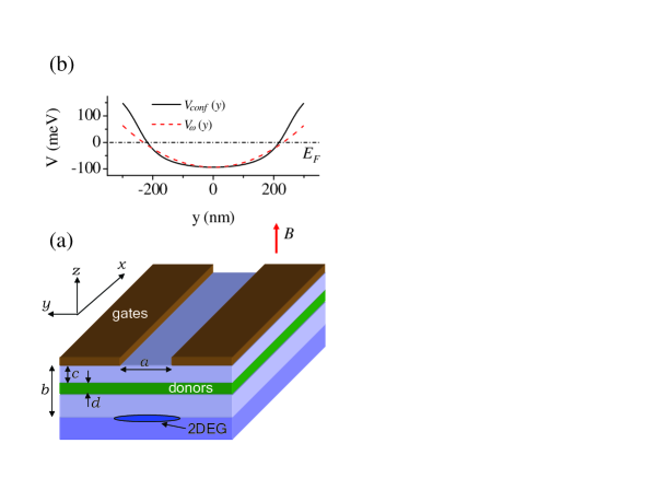
Figure 1: (Color online). (a) A schematic layout of a split-gate quantum wire in a perpendicular magnetic field. (b) Solid line: the calculated electrostatic potential $V_{conf}(y)$ for the quantum wire with $a=500$ nm, $b=60$ nm, $c=14$ nm, $d=$ 36 nm, $\rho_{d}=6\cdot 10^{23}$ m${}^{-3},$ and $|V_{0}|=0.2$ V. A dashed line shows the corresponding parabolic confinement $V_{\omega}(y)=m^{\ast}\left(\omega y\right)^{2}/2$ (with $\hbar\omega=2meV)$ often used to approximate the external electrostatic confinement.

The distance between gates is $a,$ the distance from the surface to the electron gas is $b$ (we disregard the spatial extension of the electron wave function in the $z$-direction). The donor layer with the donor density $\rho_{d}$ has the width $d$ and is situated at the distance $c$ from the surface. The external electrostatic confinement potential can be written in the form

$$V_{conf}(y)=V_{g}(y)+V_{d}+V_{Schottky},$$ (1)

where $V_{g}(y)$ and $V_{d}$ are respectively potentials due to the gatesDavies and the donor layerMartorell , and $V_{Scho}$ is the Schottky barrier,

$$V_{g} =|V_{0}|\left\{1-\frac{1}{\pi}\left[\arctan\frac{a+y}{b}+\arctan\frac{a-y}{b}\right]\right\},$$ (2)

$$V_{d} =-\frac{e^{2}}{\varepsilon_{0}\varepsilon_{r}}\rho_{d}d\left(c+d/2\right),$$ (3)

with $V_{0}$ being the (negative) applied gate voltage, and $\varepsilon_{r}$ being the dielectric constant. The Schottky potential is chosen to be $V_{Schottky}=0.8$ eV, which is appropriate for GaAs. The external electrostatic confinement potential is shown in Fig. 1 (b) for a representative quantum wire with parameters typical for an experiment. Figure 1 (b) also illustrates the corresponding parabolic potential $V(y)=\frac{m^{\ast}}{2}\left(\omega y\right)^{2}$ often used to approximate the electrostatic confinement in the split-gate wires, where $m^{\ast}$ is the effective electron mass ($m^{\ast}=0.067m_{e}$ for GaAs).

The wire is described by the effective Hamiltonian in a perpendicular magnetic field, $\mathbf{B_{\bot}}=B\mathbf{\hat{z}}$,

$$H^{\sigma}=H_{0}+V_{conf}(y)+V_{eff}^{\sigma}(y)+g\mu_{b}B\sigma,$$ (4)

where $H_{0}$ is the kinetic energy in the Landau gauge, $\mathbf{A}=(-By,0,0)$,

$$H_{0}=-\frac{\hbar^{2}}{2m^{\ast}}\left\{\left(\frac{\partial}{\partial x}-\frac{eiBy}{\hbar}\right)^{2}+\frac{\partial^{2}}{\partial^{2}y}\right\}.$$ (5)

The last term in Eq. (4) accounts for Zeeman energy where $\mu_{b}=e\hbar/2m_{e}$ is the Bohr magneton, $\sigma=\pm\frac{1}{2}$ describes spin-up and spin-down states, $\uparrow$ , $\downarrow$, and the bulk $g$ factor of GaAs is $g=-0.44.$

The effective potential, $V_{eff}^{\sigma}(y)$ within the framework of the Kohn-Sham density functional theory reads ParrYang ; Kohn_Sham ; QDOverview ,

$$V_{eff}^{\sigma}(\mathbf{r})=V_{H}(y)+V_{xc}^{\sigma}(y).$$ (6)

$V_{H}($r$)$ is the Hartree potential due to the electron density $n(y)=\sum_{\sigma}n^{\sigma}(y)$ (including the mirror charges),

$$V_{H}(y)=\frac{e^{2}}{4\pi\varepsilon_{0}\varepsilon_{r}}\int_{-\infty}^{+\infty}dx^{\prime}\int_{-\infty}^{+\infty}dy^{\prime}n(y)$$

$$\ \times\Bigg{[}\frac{1}{\sqrt{\left(x-x^{\prime}\right)^{2}+\left(y-y^{\prime}\right)^{2}}}-$$

$$-\frac{1}{\sqrt{\left(x-x^{\prime}\right)^{2}+\left(y-y^{\prime}\right)^{2}+4b^{2}}}\Bigg{]}$$

$$=-\frac{e^{2}}{4\pi\varepsilon_{0}\varepsilon_{r}}\int_{-\infty}^{+\infty}dy^{\prime}n(y^{\prime})\ln\frac{\left(y-y^{\prime}\right)^{2}}{\left(y-y^{\prime}\right)^{2}+4b^{2}}.$$ (7)

The exchange and correlation potential $V_{xc}(y)=V_{x}(y)+V_{c}(y)$ in the local spin density approximation is given by

$$V_{xc}^{\sigma}=\frac{d}{dn^{\sigma}}\left\{n^{\sigma}\epsilon_{xc}\left(n,\zeta(y)\right)\right\}$$ (8)

where $\zeta(y)=\frac{n^{\uparrow}-n^{\downarrow}}{n^{\uparrow}+n^{\downarrow}}$ is the local spin-polarization. As we mentioned in Introduction, in the present paper we use the parameterization of Tanatar and Cerperly (TC) TC ; for the sake of completeness, the explicit expressions for $V_{x}(y)$ and $V_{c}(y)$ are given in Appendix (see also Ref. [Macucci1993, ]).

III Calculation of the electron density and edge states in quantum wires.

In order to calculate the self-consistent electron densities, wave functions and wave vectors of the magneto-edge states as well as corresponding currents, we use the Green’s function technique. A detailed account of the major steps of the calculations is presented in this section.

III.1 Hamiltonian in the mixed energy-space representation.

Numerical computation of the self-consistent electron densities and other quantities of interest requires the discretization of the Hamiltonian (4). Introduce a numerical grid (lattice) with the discrete variables $m,n$ according to $x,y\rightarrow ma,na,$ where $a$ is the lattice constant. The computational domain consists of $N_{s}$ sites in the transverse $n$-direction (the wire is infinite in the longitudinal $m$-direction). Discretization of the continuous Hamiltonian (4) gives a standard tight-binding Hamiltonian with the magnetic field included in the form of the Peierls substitutionFerry ,

$$H^{\sigma} =\sum_{m}\Bigg{\{}\sum_{n=1}^{N_{s}}\left\{\epsilon_{0}+V^{\sigma}(n)\right\}a_{m,n}^{+}a_{m,n}-$$ (9)

$$-t\,\left\{a_{m,n}^{+}a_{m,n+1}+e^{-iqn}a_{m,n}^{+}a_{m+1,n}+\text{h.c.}\right\}\Bigg{\}},$$

where

$$V^{\sigma}(n)=V_{conf}(n)+V_{eff}^{\sigma}(n)+g\mu_{b}B\sigma$$ (10)

is the total confining potential, the hopping element $t=\hbar^{2}/2m^{\ast}a^{2},$ the site energy $\epsilon_{0}=4t,$ and $q=eBa^{2}/\hbar;$ $a_{m,n}^{+}$ and $a_{m,n}$ denote the creation and annihilation operators at the site $\left(m,n\right).$ The translational invariance in the longitudinal direction dictates the Bloch form for the propagating states in the quantum wire,

$$\left|\psi_{\alpha}^{\sigma}\right\rangle=\sum_{m}e^{ik_{\alpha}^{\sigma}m}\sum_{n=1}^{N_{s}}\psi_{\alpha}^{\sigma}(n)\,a_{m,n}^{+}\left|0\right\rangle,$$ (11)

where the index $\alpha$ corresponds to the $\alpha$-th Bloch state with the wave vector $k_{\alpha}^{\sigma}$ and the transverse wave function $\psi_{\alpha}^{\sigma}(n).$ In Eq. (11) the wave function $\psi_{\alpha}^{\sigma}(n)$ corresponds to the real space representation. To facilitate the numerical calculation, it is convenient to expand the wavefunctions over the transverse eigenstates (modes) of a homogeneous wire of the width of $N_{s}$ sites, $\phi_{j}(n)=\sqrt{\frac{2}{N_{s}+1}}\sin\frac{\pi jn}{N_{s}+1},$

$$\psi_{\alpha}^{\sigma}(n)=\sum_{j=1}^{N}\psi_{\alpha,j}^{\sigma}\phi_{j}(n),$$ (12)

where the expansion coefficients $\psi_{\alpha,j}^{\sigma}$ can be interpreted as the wavefunction in the “energy” representation in the space of the transverse eigenstatesZ . Note that Eq. (12) corresponds to a conventional sin-transformation, whose inverse transform is given by the same equationNum_rec . The summation in Eq. (12) runs over $1\leq j\leq N$, with $N=N_{s}.$ In practice, however, it is sufficient to limit the summation to much smaller number of modes, with $N\ll N_{s}.$ Because the speed of the method is determined by the dimension of the matrices (that is given by $N_{s}$ in the real space representation and $N$ in the “energy” representation), passing to the “energy” representation greatly enhances the computational speed. For example, for the wire of the width of 0.5 $\mu$m, it is sufficient to use $N\approx 50$ modes to achieve a good convergence of the results with respect to the mode number. At the same time, in the real space representation, $N_{s}=500$ (with the lattice constant $a=1$ nm), which makes computations rather impractical.

Passing from the real space representation to the “energy” representation in the transverse direction we arrive to the Hamiltonian in the mixed energy-space representation (i.e., in the real space representation in the longitudinal $m$-direction and “energy” representation in the transverse $n$-direction)Z ,

$$H =\sum_{m}\Bigg{\{}\sum_{j=1}^{N}\left\{\epsilon_{j}+2t\right\}a_{m,j}^{+}a_{m,j}+\sum_{j,j^{\prime}}^{N}V_{jj^{\prime}}^{\sigma}a_{m,j}^{+}a_{m,j^{\prime}}$$

$$-\sum_{j,j^{\prime}}^{N}\left[t_{jj^{\prime}}^{L}a_{m,j}^{+}a_{m+1,j^{\prime}}+t_{jj^{\prime}}^{R}a_{m+1,j}^{+}a_{m,j^{\prime}}\right]\Bigg{\}},$$ (13)

where $\epsilon_{j}=2t-2t\cos\frac{\pi j}{N+1}$ are the eigenvalues of the transverse motion corresponding to the eigenfunctions $\phi_{j}(n);$ the creation and annihilation operators in the mixed space-energy representation are related to the real space creation and annihilation operators according to $a_{m,j}^{+}=\sum_{n=1}^{N_{s}}\phi_{j}(n)a_{m,n}^{+},$ $a_{m,j}=\sum_{n=1}^{N_{s}}\phi_{j}(n)a_{m,n}$. The matrix elements of total confining potential and the hopping matrix elements read are given by

$$V_{jj^{\prime}}^{\sigma} =\sum_{n=1}^{N_{s}}\phi_{j}(n)V^{\sigma}(n)\phi_{j^{\prime}}(n),\;$$ (14)

$$t_{jj^{\prime}}^{R} =t\sum_{n=1}^{N_{s}}\phi_{j}(n)e^{iqn}\phi_{j^{\prime}}(n),\;t_{jj^{\prime}}^{L}=(t_{jj^{\prime}}^{R})^{\ast}.$$

Note that Hamiltonian (13) has nearest-neighbor couplings in the longitudinal $m$-direction (described by two last terms in Eq. (13)). In the transverse (“energy”) direction, the magnetic field couples all states $j$ on slice $m$ to all states $j\prime$ on neighboring slices $m+1$ and $m-1$. The Bloch wavefunctions (11) in the mixed space-energy representation read

$$\left|\psi_{\alpha}^{\sigma}\right\rangle=\sum_{m}e^{ik_{\alpha}^{\sigma}m}\sum_{j=1}^{N}\psi_{\alpha,j}^{\sigma}\,a_{m,j}^{+}\left|0\right\rangle.$$ (15)

III.2 Bloch states of a quantum wire in magnetic field.

Define a retarded Green’s function of the Hamiltonian $H$ in a standard wayFerry ; Datta ,

$$\left(E-H+i\varepsilon\right)G=\mathbf{1,}$$ (16)

where $\mathbf{1}$ is a unitary operator. Calculate first the Green’s function $g^{\sigma}$ corresponding to a single slice (see Fig. 2 (a)).

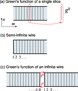
Figure 2: (Color online). Graphical illustration of the calculations of the Green’s function for a single slice (a), and for an infinite wire (b), (c).

The Hamiltonian of $m$-th single slice reads

$$h_{m}^{\sigma}=\sum_{j=1}^{N}\left\{\epsilon_{j}+2t\right\}a_{m,j}^{+}a_{m,j}+\sum_{j,j^{\prime}}^{N}V_{jj^{\prime}}^{\sigma}a_{m,j}^{+}a_{m,j^{\prime}},$$ (17)

(Note that a single slice is not coupled to its neighbors, and hence two last terms in Eq. (13) are absent in Eq. (17)). Using this operator in the definition of Green’s function (16), and taking the matrix elements $\langle 0|a_{m,j}...\,a_{m,j^{\prime}}^{+}|0\rangle,$ we arrive to the $N\times N$ system of linear equations for the matrix elements of the Green’s function of a single slice $g_{j^{\prime\prime}j^{\prime}}^{\sigma}=\langle 0|a_{m,j}\,g^{\sigma}\,a_{m,j^{\prime}}^{+}|0\rangle$,

$$\sum_{j^{\prime\prime}=1}^{N}\left(\left(E-\epsilon_{j}-2t\right)\delta_{j,j^{\prime\prime}}-V_{jj^{\prime\prime}}^{\sigma}\right)g_{j^{\prime\prime}j^{\prime}}^{\sigma}=\delta_{j,j^{\prime}}.$$ (18)

Note that because of the translational invariance, we have dropped index $m$ in the definition of the matrix element of the Green’s function of a single slice.

Knowledge of the Green’s function of a single slice $g^{\sigma}$ allows one to find the Bloch states of an infinite wire. The eigenvectors $\left\{\psi_{j\alpha}^{\sigma}\right\}$ and eigenvalues $\left\{k_{\alpha}^{\sigma}\right\}$ are determined by the eigenequationZ

$$\left(\begin{array}[c]{cc}-\left(g^{\sigma}t^{L}\right)^{-1}&-\left(t^{L}\right)^{-1}t^{R}\\ 1&0\end{array}\right)\left(\begin{array}[c]{c}e^{ik}\overrightarrow{\psi^{\sigma}}\\ \overrightarrow{\psi^{\sigma}}\end{array}\right)=e^{ik}\left(\begin{array}[c]{c}e^{ik}\overrightarrow{\psi^{\sigma}}\\ \overrightarrow{\psi^{\sigma}}\end{array}\right),$$ (19)

where the matrixes $t^{R},t^{L}$ and $g^{\sigma}$ have matrix elements given by Eqs. (14) and (18) respectively, and $\overrightarrow{\psi^{\sigma}}$ is the column vector composed of $\psi_{j}^{\sigma},$ $1\leq j\leq N$ (Eq. (12)). Here and hereafter we use Greek indexes $\alpha,$ $\alpha^{\prime}$ for Bloch states of the wire, and Roman indexes $j,j^{\prime}$ for the basis set of the transverse eigenfunctions $\left\{\phi_{j}(n)\right\}$. Equation (19) has $2N$ eigenvalues $k_{\alpha}^{\sigma},$ $1\leq\alpha\leq N$, which can be real or complex, describing respectively propagating and evanescent states (Here and hereafter $k_{\alpha}^{\sigma}$ is given in units of $a^{-1}$ and the group velocity $v$ is in units of $a)$. The eigenvalues corresponding to right propagating states ($v=\,\partial E/\partial k>0,$ $\Im(k)=0$) and states decaying to the right ($\Im(k)>0$) we denote by $k_{\alpha}^{\sigma^{+}}$ with corresponding eigenstates $\psi_{j\alpha}^{\sigma^{+}}$. Correspondingly, $k_{\alpha}^{\sigma^{-}}$ and $\psi_{j\alpha}^{\sigma^{-}}$ stand for left propagating states ($v=\,\partial E/\partial k<0,$ $\Im(k)=0$) and states decaying to the left ($\Im(k)<0$). Sorting right- and left-propagating eigenstates can be easily done by calculating their group velocityZ

$$v_{\alpha}^{\sigma}=\frac{1}{\hbar}\frac{\partial E}{\partial k_{\alpha}^{\sigma}}=-\frac{2}{\hbar}\sum_{j,j^{\prime}}^{N}\left(\psi_{j\alpha}^{\sigma}\right)^{\ast}\psi_{j^{\prime}\alpha}^{\sigma}\Im\left[e^{-ik_{\alpha}^{\sigma}}t_{jj^{\prime}}^{L}\right].$$ (20)

Passing to the real space representation for the wave functions in the above expressions and using the quantum-mechanical particle current density for $\alpha$-th Bloch state calculated in a standard way for a tight-binding latticeZ ,

$$j_{\alpha}^{\sigma}(n,E)=\frac{2t}{\hbar}\sin\left(qn+k_{\alpha}^{\sigma}\right)|\psi_{\alpha}^{\sigma}(n)|^{2},$$ (21)

the group velocity (20) can be expressed as the total particle current of $\alpha$-th Bloch state,

$$v_{\alpha}^{\sigma}=\sum_{n}j_{\alpha}^{\sigma}(n,E).$$ (22)

To conclude this section we note that a direct calculation of the eigenvectors $k_{\alpha}^{\sigma}$ and eigenfunctions $\psi_{j^{\prime}\alpha}^{\sigma}$ by substitution of Eq. (15) into Schrödinger equation and calculation of the roots of the corresponding determinant is possible (see e.g., Refs. Ando_1993, ; Tejedor, ; Gerhardts_2004, ). However, the procedure used here is more efficient as the solution of the eigenproblem (19) is numerically faster and less demanding than the root searching. Besides, an important advantage of the present method is that it can be directly incorporated into magnetotransport calculations, because in contrast to the root searching method, the present technique provides the eigenstates and wave vectors at the given energy, not at a given wavevector.

III.3 Calculation of the local electron density.

The diagonal elements of the total Green’s function of an infinite wire in the real space representation give the local density of states (LDOS) at the site $\mathbf{r}=(m,n)\cite[cite]{\@@bibref{Authors Phrase1YearPhrase2}{Datta}{\@@citephrase{(}}{\@@citephrase{)}}},$

$$\rho^{\sigma}(\mathbf{r},E)=-\frac{1}{\pi}\Im\left[G^{\sigma}(\mathbf{r},\mathbf{r},E)\right].$$ (23)

The LDOS $\rho^{\sigma}(\mathbf{r},\mathbf{r},E)$ can be used to calculate the local electron density at the site $\mathbf{r}$,

$$n^{\sigma}(\mathbf{r})=\int_{V_{b}}^{\infty}dE\,\rho^{\sigma}(\mathbf{r},E)f(E-E_{F}),$$ (24)

where $f(E-E_{F})$ is the Fermi-Dirac distribution function and the lower limit of integration $V_{b}$ corresponds to the bottom of the total confining potential. Note that $\rho^{\sigma}(\mathbf{r},\mathbf{r},E)$ is a rapidly varying function of energy diverging as $\sim\left(E-E_{\alpha}\right)^{-1/2}$ when $E$ approaches the threshold subband energies $E_{\alpha}$. Because of this, a direct integration along the real axis is rather ineffective as its numerical accuracy is not sufficient to achieve convergence of the self-consistent calculation of the electron density . We therefore calculate integral (24) by transforming the integration contour into the complex energy plane $\Im\left[E\right]>0$ where the Green’s function is much more smoother than on the real axis. (Note that all poles of the Green’s function (23) are in the lower half-plain $\Im\left[E\right]<0$). A typical contour used in the integration avoiding poles of the Fermi-Dirac function $f(E-E_{F})$ is shown in Fig. 3.

Figure 3: A typical integration contour used in the calculation of integral (24). Dots indicate the poles of the Fermi-Dirac distribution function in the upper complex plane at $\Re\left[E\right]=E_{F}$, $\Im\left[E\right]=(2m+1)\pi kT,$ $m=0,1,2,\ldots$ .

We calculate the diagonal elements of the total Green’s function $G^{\sigma}(\mathbf{r},\mathbf{r},E)$ as follows. We start from a semi-infinite quantum wire and calculate its surface Green’s function $\Gamma$ (i.e. Green’s function for the boundary slice $m=1$), see Fig. 2 (b). The right and left surface Green’s functions $\Gamma^{r}$ and $\Gamma^{l}$ (corresponding to a semi-infinite wires open respectively to the right and left) can be written in a matrix formAndo_Gamma ; Z

$$\Gamma_{\sigma}^{r}t^{R} =-\Psi_{\sigma}^{+}K_{\sigma}^{+}\Psi_{\sigma}^{+^{-1}}$$ (25)

$$\Gamma_{\sigma}^{l}t^{L} =-\Psi_{\sigma}^{-}\left(K_{\sigma}^{-}\right)^{-1}\left(\Psi_{\sigma}^{-}\right)^{-1},$$

where the matrix elements $(\Psi_{\sigma}^{+(-)})_{j\alpha}=$ $\psi_{j\alpha}^{\sigma^{+(-)}},$ $(K_{\sigma}^{+(-)})_{\alpha\alpha^{\prime}}=\exp\left(k_{\alpha}^{\sigma^{+(-)}}\right)\delta_{\alpha\alpha^{\prime}}.$ We then connect this semi-infinite wire to the second semi-infinite wire to form an infinitely long quantum wire as shown in Fig. 2 (c). The total Green’s function can be calculated with the help of Dyson equationFerry ; Datta

$$G=G^{0}+G^{0}UG,$$ (26)

where $G^{0}$ correspond to the “unperturbed” structures (the left and right semi-infinite wires), and the operator $U$ describes the interaction between them,

$$U=-\sum_{j,j^{\prime}}^{N}\left[t_{jj^{\prime}}^{L}a_{0,j}^{+}a_{1,j^{\prime}}+t_{jj^{\prime}}^{R}a_{1,j}^{+}a_{0,j^{\prime}}\right],$$ (27)

(see Eq. (13)). Using Eq. (26) to calculate the matrix element $(G^{\sigma})_{jj^{\prime}}=\langle 0|a_{1,j}\,G^{\sigma}\,a_{1,j^{\prime}}^{+}|0\rangle$, we obtain Green’s function for the slice $m=1$ (Note that because of the translational invariance in the $m$-direction, the calculated Green’s function is the same for all slices),

$$G^{\sigma}=\left(\mathbf{1}-\Gamma_{\sigma}^{r}t^{R}\Gamma_{\sigma}^{l}t^{L}\right)^{-1}\Gamma_{\sigma}^{r},$$ (28)

where $\mathbf{1}$ is the unit matrix. Note that Eq. (28) gives Green’s functions in the “energy” representation of the space of the transverse eigenstates. To obtain the Green’s function in the real space representation needed to compute the electron density $n^{\sigma}(\mathbf{r})$ (24) we perform a standard change of the basis, $G^{\sigma}(n,n,E)=\sum_{j,j^{\prime}}^{N}\varphi_{j}(n)G_{jj^{\prime}}^{\sigma}\varphi_{j^{\prime}}(n).$

III.4 Self-consistent calculations

Iteration procedure. We calculate magneto-edge states and electron densities in a quantum wire in a self-consistent way, when on each iteration step a small part of a new potential (10) is mixed with the old one (from the previous iteration step),

$$V_{i+1}^{\sigma}(n)=(1-\epsilon)V_{i}^{\sigma}(n)+\epsilon\,V_{i+1}^{\sigma}(n),$$ (29)

$\epsilon$ being a small constant, $\sim 0.1-0.01$. Using this input potential we, for a given energy $E,$ solve the eigenproblem (19) to find the Bloch states in the quantum wire. (Note that energy $E$ is chosen in the complex plane as shown in Fig. (3)). We then use the obtained results to calculate the Green’s function $G^{\sigma}(n,n,E)$ according to Eqs. (25)-(28). The integration of the Green’s function (24) gives the electron densities $n^{\sigma}(\mathbf{r})$, which are subsequently used to compute the new total confining potential (10). It is typically needed $\sim 1000$ iteration steps to achieve our convergence criterium $|n_{1D}^{i+1}-n_{1D}^{i}|/(n_{1D}^{i+1}+n_{1D}^{i})<10^{-5},$ where $n_{1D}^{i}$ is the one dimensional electron density $n_{1D}=\int n(\mathbf{r})\,dy\,$ on $i$-th iteration step.

Adjustment of the Fermi energy. When the same fixed Fermi energy $E_{F}$ is used for different magnetic fields $B$, the calculated self-consistent one dimensional electron density changes as $B$ varies. Depending on a particular realization of a quantum wire, one might need to adjust $E_{F}$ for each $B$ in order to keep the total electron density fixed, as magnetic field does not change the electron density in the system. However, in a typical experimental situation when a long quantum wire is connected to a 2DEG Wrobel , the Fermi energy in the reservoirs (not the electron density in the wire) is fixed. Because of this, in all calculations reported in the paper we keep $E_{F}$ fixed (we set $E_{F}=0$).

Note that we have also performed calculations where $E_{F}$ was adjusted to keep the electron density $n_{1D}^{\sigma}$ constant. All the results obtained in this case (in particularly, the density and current spin polarizations) are qualitatively and quantitatively similar to those obtained in the case when $E_{F}$ is adjusted.

Bloch states, subband structure and current density. Having calculated the total self-consisted confining potential, we can compute the Bloch wave functions and wave vectors by solving the eigenequation (19) for the whole range of energies of interest (note that for these calculations the energy has to be chosen on the real axis). Knowledge of the wave vectors for different states allows us to recover the subband structure, i.e. to calculate an overage position $x_{\alpha}^{\sigma}$ of the wave functions for different modes $\alpha$Davies_book ,

$$x_{\alpha}^{\sigma}=\frac{\hbar k_{\alpha}^{\sigma}a}{eB}.$$ (30)

We calculate the conductance of the wire $G^{\sigma}=I^{\sigma}/V$ on the basis of the linear-response Landauer formula,

$$I^{\sigma}=\frac{e^{2}}{h}V\sum_{\alpha}\int_{E_{th\,\alpha}^{\sigma}}^{\infty}dE\left(-\frac{\partial f\left(E-E_{F}\right)}{\partial E}\right),$$ (31)

where summation is performed over all propagating modes $\alpha$ for the spin $\sigma,$ with $E_{th\,\alpha}^{\sigma}$ being the propagation threshold for $\alpha$-th mode. In order to visualize the current density we can re-write Eq. (31) for the total current in the form $I_{\alpha}^{\sigma}=a\sum_{n}J_{\alpha}^{\sigma}(n)\,$, where the current density for the mode $\alpha$ reads

$$J_{\alpha}^{\sigma}(n)=\frac{e^{2}}{h}V\int dE\frac{j_{\alpha}^{\sigma}(n,E)}{v_{\alpha}^{\sigma}}\left(-\frac{\partial f\left(E-E_{F}\right)}{\partial E}\right),$$ (32)

with $v_{\alpha}^{\sigma}$ and $j_{\alpha}^{\sigma}(n,E)$ being respectively the group velocity and quantum-mechanical particle current density for the state $\alpha$ at the energy $E$ (see Eqs. (22),(21)), and $V$ being the applied voltage.

IV Results and discussion

IV.1 Hartree approximation

To outline the role of exchange and correlation interactions we first study the magnetotransport in a quantum wire within the Hartree approximation (i.e., when $V_{xc}^{\sigma}(y)$ is not included in the effective potential (6), and the spin polarization is driven by Zeeman splitting of the energy levels). In our calculations we use the parameters of a quantum wire indicated in Fig. 1, and the temperature $T=1$K. With these parameters the effective width of the wire is $\sim 400$nm, and the sheet electron density $n\approx 1.5\cdot 10^{15}m^{-2}$. Figure 4 (a) shows the one-dimensional (1D) electron density $n_{1D}^{\sigma}$ for the spin-up and spin-down electrons in the quantum wire. The pronounced feature of this dependence is a $1/B$-periodic, loop-like pattern of the density spin polarization $P_{n}=\frac{n_{1D}^{\uparrow}-n_{1D}^{\downarrow}}{n_{1D}^{\uparrow}+n_{1D}^{\downarrow}}$ as illustrated in Fig. 4 (b).

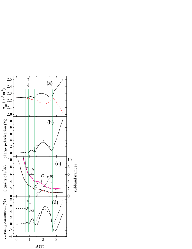
Figure 4: (Color online). (a) One-dimensional charge density for the spin-up and spin-down electrons, $n_{1D}^{\uparrow},n_{1D}^{\downarrow}$ in the Hartree approximation, and (b) spin polarization of the charge density, $P_{n}=\frac{n_{1D}^{\uparrow}-n_{1D}^{\downarrow}}{n_{1D}^{\uparrow}+n_{1D}^{\downarrow}}$, as a function of magnetic field $B$. (c) Total number of subbands, conductance of the spin-up and spin-down electrons, the total conductance $G=G^{\uparrow}+G^{\downarrow}$, and the filling factor in the center of the wire $\nu(0)$ (note $G_{\mathrm{Ch}}=\frac{e^{2}}{h}\nu(0)$. (d) The spin polarization of $G$ and $G_{\mathrm{Ch}}$. Parameters of the wire are chosen as indicated in the caption to Fig. 1. Arrows in (b) indicate the magnetic fields corresponding to the magnetosubband band structure shown in Fig. 5. Temperature $T=1$K.

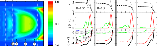
Figure 5: (Color online). (a) Spatially resolved difference in the electron densities $n^{\uparrow}(y)-n^{\downarrow}(y)$ as a function of $B$ calculated within Hartree approximation. (b)-(e) The subband structure for the magnetic fields indicated in (a) (see also Fig. 4 (b)). Upper panel: The filling factor $\nu(y)$ for spin-up and spin-down electrons. Middle panel: the current density distribution for spin-up and spin-down electrons calculated according to Eq. (32). Lower panel: magnetosubband structure for spin-up and spin-down electrons (solid and dashed lines correspondingly). Fat solid and dashed lines indicate the total confining potential, Eq. (10), for respectively spin-up and spin-down electrons. Temperature $T=1$K.

Figure 4 (c) shows the number of spin-resolved subbands as a function of $B.$ (As the calculations are done for the finite temperature $T,$ for a given magnetic field, we count the subbands that lie in the energy interval $E\lesssim E_{F}+4kT,$ where $4kT$ determines the energy window beyond which the Fermi-Dirac distribution rapidly decays to zero). The pronounced feature of this dependence is that the number of subbands is always even, $N=2,$ 4, 6, … , such that the spin-up and spin-down subbands depopulate simultaneously. The comparison of Figs. 4 (a)-(c) demonstrates that the spin polarization is directly related to the magnetosubband structure: The polarization drops almost to zero at the magnetic fields when the subbands depopulate. In order to understand the origin of the spin polarization let us analyze the evolution of the subband structure as the applied magnetic field varies. Let us concentrate at the polarization loops in the field interval $1.3T\lesssim B\lesssim 2.6T$ when the number of the spin-resolved subbands $N=4$ and the filling factor in the middle of the wire $2\leq\nu(0)\leq 4$.

Figure 5 (a) shows the spatially resolved difference in the electron densities $n^{\uparrow}(y)-n^{\downarrow}(y)$ as a function of $B.$ When the subband number $N\geq 4$ (for $B\lesssim 2.6T$), the electron density is mostly polarized in the inner region of the wire. We thus concentrate first on the formation of the compressible and incompressible strips in the inner region due to the upper subband. Figure 5 (b) shows the filling factor $\nu^{\sigma}(y),$ current densities $J_{\alpha}^{\sigma}(n),$ and the magnetosubband structure for the magnetic field $B=1.35T.$ This field corresponds to the case when the 5th and 6th spin-resolved subbands just became depopulated, i.e. their bottoms are situated at $\gtrsim E_{F}+4kT$ . The 3rd and 4th subbands are separated from the 5th and 6th by the distance $\hbar\omega_{c}$ (with $\omega_{c}$ being the cyclotron frequency, $\hbar\omega_{c}\gg kT$), see Fig. 5 (b). They are therefore situated below the Fermy energy and are fully populated. As the results, the electron density is constant, which corresponds to the formation of the incompressible strip. Because of the spin-up and down subbands are fully filled, the corresponding electron densities are equal and the spin polarization of the electron density is zero.

When magnetic field is raised the subbands are pushed up in the energy and the two highest spin-resolved subbands, following Chklovslii et al. scenarioChklovskii , become pinned at the Fermi energy. The subband bottoms flatten which signals the formation of the compressible strip in the middle of the wire, see Fig. 5 (c). When the subband bottoms reach the energy $E\approx E_{F}-4kT$ , the subbands become partially occupied. Partial subband occupation combined with their energy separation due to Zeeman interactions results in the different population for spin-up and down electrons. With increase of the magnetic field the filling factor decreases, but spin polarization increases until the subband bottoms approach $\sim E_{F}$, Fig. 5 (d). This magnetic field corresponds to the maximal spin polarization $P_{n}\sim 3\%$. With further increase of the magnetic field, the subbands bottoms are pushed up above $E_{F},$ which causes further decrease of the filling factor and diminishing screening efficiency. As the result, the width of the compressible strip decreases until the upper subbands become completely depopulated and the incompressible strip forms again in the middle of the wire, see Fig. 5 (e). This is accompanied by a gradual decrease of the density polarization $P_{n}$ to zero. The shrinkage of the compressible strip in the middle of the wire can be also clearly traced in the evolution of the current density distribution, shown in the middle panels of Figs. 5 (b)-(e). It is interesting to note that the compressible regions are not formed for the outermost edge states corresponding to the lowest subbands $N=1$ and 2. This is because that in the field interval under study the extension of the wave function is larger than the width of the compressible strip predicted by the Chklovskii et al. theoryChklovskii . The onset of the formation of the compressible strips can be seen in Fig. 5 (e) for $B=2.5T.$ Note that the effect of the formation/non-formation of the compressible strips in quantum wires was discussed in details by Suzuki and Ando for the case of spinless electronsAndo_1998 .

The described above picture of evolution of the density polarization qualitatively holds for all other polarization loops. We stress that in all the loops only two upper, partially occupied spin-resolved subbands contribute to the spin polarization, whereas remaining subbands are fully (and equally) populated and thus do no contribute to the total spin polarization. When magnetic field exceeds $B=2.6T,$ only two subbands survive in the quantum wire. With further increase of magnetic field the upper (spin-up) subband gradually depopulates and the density polarization $P_{n}$ grows linearly until it reaches 100% when only the spin-down subband remains in the wire.

It should be also stressed that within Hartree approximation two outermost spin-up and spin-down edge states are not spatially polarized (i.e. they are situated at a practically same distance from the wire edges, see Fig. 5).

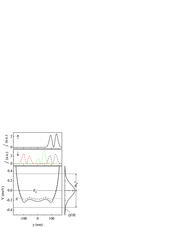
Figure 6: (Color online) Lower panel: A closeup of the spin-up and spin-down subbands $N=3,4$ (solid and dashed lines respectively) for the magnetic field $B=1.5T$, when the polarization of the conductance $P_{G}$ is negative. Upper panels: current density distribution for the spin-up and spin-down electrons at the energy $E$ indicated in the lower panel. At this energy, there is one propagating state for spin-up electrons and three propagating states for spin-down electrons. Left inset shows the derivative of the Fermi-Dirac distribution determining the weight of the contributions from the current-carrying states to the total current density at the given energy, see Eq. (32).

Figures 4 (c),(d) show the conductance $G^{\sigma}$ for spin-up and spin-down states and its relative spin polarization $P_{G}=\frac{G^{\uparrow}-G^{\downarrow}}{G^{\uparrow}+G^{\downarrow}}.$ The spin polarization $P_{G}$ follows a similar behavior as the density polarization $P_{n}$ with one subtle difference. Namely, the density polarization $P_{n}$ is always positive because spin-up states always lie in energy below the corresponding spin-down states, and, therefore $n^{\uparrow}(y)-n^{\downarrow}(y)>0.$ In contrast, the spin polarization of the current, after reaching zero, does not immediately raises as the magnetic field increases, but, instead, becomes negative before raising again. Note that this is accompanied by a small (but noticeable) increase of the total current (at $B\sim 1.5T,$ $3T,$ see Figs. 4 (c)). This effect can be traced back to the self-consistent band structure as explained below. Figure 6 shows a closeup of the upper subbands $N=3,4$ for the magnetic field $B=1.5T$, i.e. when the current polarization is negative. Because the spin-up/down subbands are not flat, for certain energies $E<E_{F}$ the upper (spin-down) subband can give rise to several propagating states, whereas the lower (spin-up) subband corresponds to only one propagating state, see Fig. 6. According to the Landaulet formula (31) all propagating states contribute equally to the total current. Because of this and due to the fact that the spin-down subband is situated closer to the Fermi energy, the total current for the spin-down electrons is larger than the current for the spin-up ones. This explains the negative spin polarization of the current and the increase of the total current at the magnetic fields just above the subband depopulation. We are not aware of the discussion of this effect in the current literature. The available experimental data, see e.g., Fig. 2 of Ref. Wrobel, showing a nonmonotonic dependence of the conductance of a quantum wire as a function of magnetic field, are consistent with the predicted behavior of the total current. Note that this feature in the conductance also survives within the DFT approach (see below, Fig. 7).

Figures 4 (c) and (d) also show the conductance and its spin polarization calculated according to the Chklovskii et al. prescription Chklovskii , $G_{\mathrm{Ch}}=\frac{e^{2}}{h}\nu(0),$ with $\nu(0)$ being the filling factor in the center of the wire. $G_{\mathrm{Ch}}$ follows the exact conductance rather good, but does not recover the steps in the conductance related to the subband depopulation (see Ref. [Gerhardts_1994 ] for a related discussion). $G_{\mathrm{Ch}}$ does not also reproduce the increase of the current and the negative conductance polarization discussed above because these features are related to the quantum-mechanical band structure.

As we mentioned before, the Hartree approximation predicts that spin-up and spin-down subbands depopulate simultaneously and thus the conductance drops in steps of $2e^{2}/h$ as the magnetic field increases. This is in strong disagreement with the experimental observations that demonstrate that the subbands depopulate one by one such that the conductance decreases in steps of $e^{2}/h.$ We will show in the next section that accounting for the exchange and correlation interactions leads to qualitatively new features in the subband structure and brings the theory to a close agreement with experiment.

IV.2 Density functional theory in the local spin density approximation

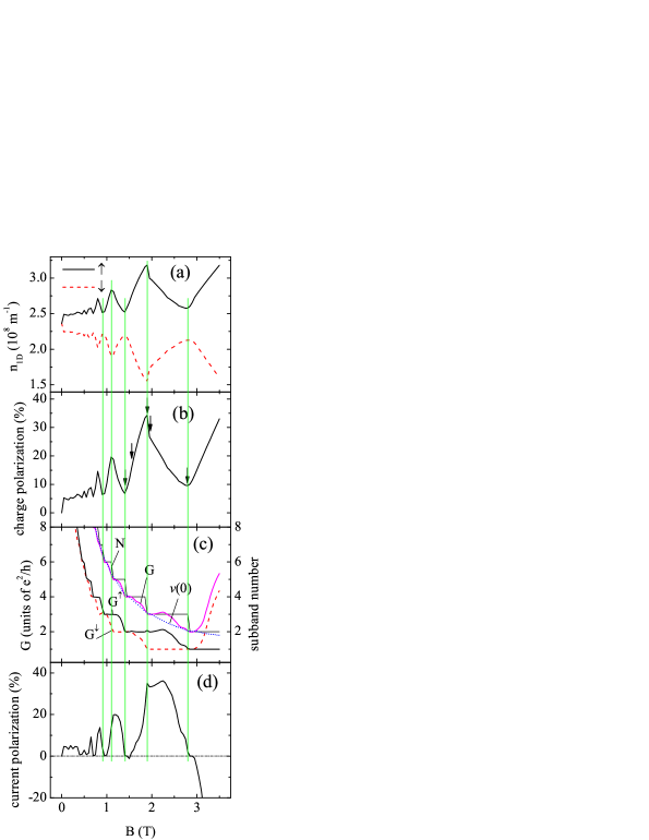
Figure 7: (Color online). (a) One-dimensional charge density for the spin-up and spin-down electrons, $n_{1D}^{\uparrow},n_{1D}^{\downarrow}$ calculated within DFT+LSDA, and (b) spin polarization of the charge density, $P_{n}=\frac{n_{1D}^{\uparrow}-n_{1D}^{\downarrow}}{n_{1D}^{\uparrow}+n_{1D}^{\downarrow}}$, as a function of magnetic field $B$. (c) Total number of subbands, conductance of the spin-up and spin-down electrons, the total conductance $G=G^{\uparrow}+G^{\downarrow}$, and the filling factor in the center of the wire. (d) The spin polarization of the conductance $P_{G}$. Parameters of the wire are chosen as indicated in the caption to Fig. 1. Arrows in (b) indicate the magnetic fields corresponding to the magnetosubband band structure shown in Fig. 8. Temperature $T=1$K.

Figures 7,8 show the electron density, conductance and subband structure for the quantum wire calculated using DFT within LSDA, Eqs. (4)-(8). Utilization of the DFT+LSDA leads to several major quantitative and qualitative differences in comparison to the Hartree approximation. First, the spin polarization of the electron density also shows a pronounced $1/B$-periodic loop-like pattern. However, for the given magnetic field $B$ the spin polarization in the quantum wire calculated on the basis of DFT is of the order of magnitude higher in comparison to the Hartree approximation. Second, the magnetosubbands depopulate one by one, and the conductance decreases in steps of $e^{2}/h$ (not in steps of $2e^{2}/h$ as in the case of Hartree approach when the spin-up and spin-down subbands depopulate simultaneously). Third, the outermost edge states become spatially polarized (separated), which is in the strong contrast with the Hartree approximation, where they are situated practically at the same distance from the wire boundary.

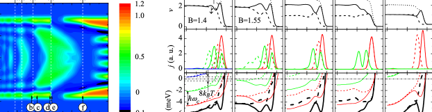
Figure 8: (Color online). (a) Spatially resolved difference in the electron densities $n^{\uparrow}(y)-n^{\downarrow}(y)$ as a function of $B$ calculated within DFT+LSDA. (b)-(e) The subband structure for the magnetic fields indicated in (a) (see also Fig. 7 (b)). Upper panel: The filling factor $\nu(y)$ for spin-up and spin-down electrons. Middle panel: the current density distribution for spin-up and spin-down electrons calculated according to Eq. (32). Lower panel: magnetosubband structure for spin-up and spin-down electrons (solid and dashed lines correspondingly). Fat solid and dashed lines indicate the total confining potential, Eq. (10), for respectively spin-up and spin-down electrons. Temperature $T=1$K.

In order to understand the effect of the exchange and correlation interactions on the evolution of the magnetosubband structure, let us now concentrate on the same field interval as studied in the previous section, i.e. when the number of the subbands lies in the interval $3\leq N\leq 4$ and the filling factor in the middle of the wire $2\leq\nu(0)\leq 4$, see Fig. 7. We start from the magnetic field $B=1.4$T, where the spin polarization of the density is minimal. Similarly to the case of Hartree approximation (Fig. 5 (b)), this corresponds to the case when 5th subbands just became depopulated as shown in Fig. 8 (b). However, in contrast to the Hartree approximation, where the Zeeman interaction is not strong enough to cause any significant spin polarization, in the present case the exchange interaction leads to a non-negligible spin polarization near the boundaries of the wire ($P_{n}\sim 7\%$). For this magnetic field the number of subbands is even, and the spin-up and spin-dow subbands are fully filled in the center of the wire. As the result, the electron densities are constant, which corresponds to a formation of the incompressible strip in the center of the wire. Because the spin-up and spin-down subbands are equally occupied, spin polarization in the center of the wire is zero (Fig. 8 (a)).

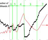
Figure 9: (Color online). Spatial separation between the outermost spin-up and spin-down edge states as a function of magnetic field $B$. (The separation between the edge states is extracted from the corresponding current distribution, see Fig. 8, middle panel). The number of subbands and the electron density spin polarization $P_{n}$ from Fig. 7 is shown for comparison.

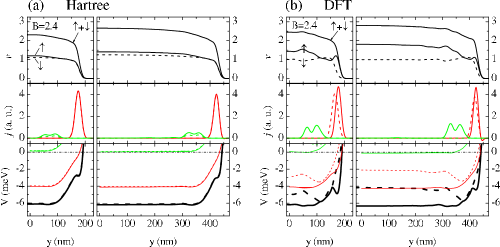
Figure 10: (Color online). The filling factor, current densities and the magnetosubband structure (upper, middle and lower panels correspondingly) calculated within Hartree and DFT approximations for two quantum wires with different distances between the gates, (a) $a=500$ nm, and (b) $a=1\mu m$. Remaining parameters of the wire are chosen as indicated in the caption to Fig. 1. Solid and dashed lines correspond to the spin-up and spin-down states. Fat solid and dashed lines indicate the total confining potential, Eq. (10), for respectively spin-up and spin-down electrons. Temperature $T=1$K.

When the magnetic field increases, all the subbands are pushed up in energy, and 4th subband gets pinned at $E_{F}$ near the boundary of the wire, forming the compressible strip, Fig. 8 (c). With increase of magnetic field, the compressible strip extends to the center of the wire, compare Figs. 8 (b) and (c). Note that in the Hartree case the separation between the subbands caused by the Zeeman splitting is small ($\ll kT$) and hence both the subbands are pinned at $E_{F}$ (see Fig. 5 (c)-(e)). In contrast, in the present case only one of the subbands is pinned at $E_{F}$ because the subband separation is determined by the exchange interaction whose magnitude can be comparable to $\hbar\omega_{c}.$

Figure 8 (d) shows the subband structure for the magnetic field $B=1.9$T when the spin polarization of the electron density is maximal. In this case 4th subband is about to be depopulated and all the remaining subbands (two spin-up and one spin down) lie below $E_{F}.$ They are therefore fully populated (2$n_{1D}^{\downarrow}\approx n_{1D}^{\uparrow}$), which corresponds to the calculated polarization $P_{n}\sim 33\%$.

When magnetic field is increased by only 0.05T, the density spin polarization drops by $\sim 10\%$, and the subband structure experiences dramatic changes, see Fig. 8 (e). In particularly, the spatial separation between the outermost spin-up and spin-down states collapses from $\sim 20$ nm to zero, as shown in Fig. 9. The explanation of this remarkable effect is based on the fact that the electrostatic energy is dominant for the system at handChklovskii . This is illustrated in Fig. 10 which compares the electron densities and the magnetosubband structure in a quantum wire calculated within the Hartree and DFT approximations for some representative value of the magnetic field. As expected, the total electron density is practically the same in the both approximations. At the same time, the magnetosubbands and the spin-up and spin-down densities vary significantly between them. It is also interesting to note that the magnetic fields corresponding to the depopulation of even subbands $N=2,4,6\ldots$ are practically the same with and without accounting for the exchange and interaction terms, compare Figs. 4 (c) and 7 (c). The dramatic changes in the subband structure at $B\sim 1.95$ T can be explained as follows. At $B\sim 1.9$T the electron density near the edge of the wire is dominated by spin-up electrons, see 7 (d), the upper and middle panels. When magnetic field is raised, 4th subband practically depopulates, and 3rd (spin-up) subbands is pushed up in energy. As the result, the density of the spin-up electrons associated with this subband is redistributed towards the center of the wire. However, this small change in the magnetic field can not affect the total density. Because of this, the density of the remaining electrons has to be adjusted to keep the total density unchanged. This can be done only if the spin-down electrons associated with the subband $N=2$ are redistributed towards the edge of the wire. As a consequence of this redistribution, the densities of the spin-up (1st subband) and spin-down (2nd subband) electrons near the wire edge become approximately equal and so does the total confining potential $V^{\sigma}(n)$, Eq. (10). The latter results in the absence of the spatial separation for the outermost edge states $N=1$ and $N=2.$ Note that the effect of a collapse of the spatial separation between the outermost edge states is related to the features of the quantum-mechanical band structure, and hence is absent in the Thomas-Fermi approximationDempsey ; Stoof . This effect can be utilized in spintronics devices operating in the edge state regime for injection of different spin speciesAndy .

The outermost spin-up and spin-down edge states remains spatially degenerate up to the magnetic field $B\sim 2.25$ T, see Fig 8 (a) and Fig. 9. The spin polarization of the electron density $P_{n}$ gradually decreases in the range $1.9$T$<B<2.8$T. This decrease is related to the gradual depopulation of the 3rd (spin-up) subband. At $B\sim 2.8$T this subband practically depopulates, $P_{n}$ reaches its minimum, and the incompressible strip is again formed in the middle of the wire (Fig. 8 (f)). With further increase of the magnetic field, 2nd (spin-up) subband gets pinned to $E_{F},$ and $P_{n}$ gradually increases until it reaches 100% at the magnetic field when the spin-up subband depopulates.

As in the case of Hartree approximation, the evolution of the magnetosubband structure within DFT described above qualitatively holds for all other polarization loops.

Figure 7(c) shows the conductance for spin-up and spin-down electrons $G^{\uparrow},G^{\downarrow}$, the total conductance $G=G^{\uparrow}+G^{\downarrow},$ the filling factor in the middle of the wire $\nu(0),$ and the spin polarization of the conductance. The total conductance $G(B)$ decreases in steps of $e^{2}/h$ closely following the depopulation of the magnetosubbands as $B$ increases. Note that the magnitude of $G(B)$ in plateau regions when $N>2$ shows slight increase in comparison to the corresponding value of $Ne^{2}/h$. This effect has the same origin as in the case of Hartree approximation (see Fig. 6 and a related discussion in the text). For $N\leq 2$ this effect becomes much more pronounced in comparison to the Hartree approximation. This is because for magnetic fields corresponding to $N\leq 2,$ the separation between bottoms of spin-up and spin-down subbands due to the exchange interaction exceeds $8kT.$ Because the subbands are not flat, the spin-down subband (which is pinned to $E_{F})$ gives rise to several states propagating in the bulk of the wire as discussed in the previous section, whereas the spin-up subband (whose bottom lies well below $E_{F})$ corresponds to only one propagating state situated near the wire edge.

Note that the propagating states giving rise to the conductance for $N\leq 2$ are the Bloch states of an infinite quantum wire. In a typical experimental condition, a long quantum wire is connected to a much wider region of 2DEGWrobel . The edge states in the region of 2DEG are coupled only to the edge states in the wire. As the results, the measured conductance for $N\leq 2$ does not exhibits the increase over the plateau values of $Ne^{2}/h$ Wrobel .

Finally, we note that our analysis of the spin polarization and evolution of magnetosubbands in quantum wires was concentrated on a representative wire with the distance between the gates $a=500$ nm and the sheet electron density $n\approx 10^{15}m^{-2}.$ We would like to emphasize that all the results presented here qualitatively hold for wires of arbitrary widths and electron densities. This is illustrated in Fig. 10 for the case of two quantum wires with different distances between the gates, $a=500$ nm and $a=1\mu m,$ which shows practically identical subband structure as well as electron and current densities distributions.

V Conclusion

In the present paper we provide a quantitative description of the structure of edge states in split-gate quantum wires in the integer quantum Hall regime. We start with a geometrical layout of the wire and calculate self-consistently quantum-mechanical magnetosubband structure and spin-resolved edge states where electron- and spin interactions are included within the density functional theory in the local spin density approximation (DFT+LSDA).

We develop an effective and stable numerical method based on the Green’s function technique capable of dealing with a quantum wire of arbitrary width in high perpendicular magnetic field. The advantage of this technique is that it can be directly incorporated into magnetotransport calculations, because it provides the eigenstates and wave vectors at a given energy, not at a given wavevector (as conventional methods do). Another advantage of this technique is that it calculates the Green’s function of the wire, which can be subsequently used in the recursive Green’s function technique widely utilized for magnetotransport calculations in lateral structures.

We use the developed method to calculate the self-consistent subband structure and propagating states in the quantum wires in perpendicular magnetic field. We discuss how the spin-resolved subband structure, the current densities, the confining potentials, as well as the spin polarization of the electron and current densities evolve when an applied magnetic field varies. We demonstrate that the exchange and correlation interactions dramatically affect the magnetosubbands in quantum wires bringing about qualitatively new features in comparison to a widely used model of spinless electrons in Hartree approximation. These features can be summarized as follows.

(a) The spin polarization of the electron density shows a pronounced $1/B$-periodic loop-like pattern, whose periodicity is related to the subband depopulation. For a given magnetic field $B$ the spin polarization in the quantum wire calculated on the basis of DFT+LSDA is of the order of magnitude higher in comparison to the Hartree approximation (where the spin polarization is driven by the Zeeman interaction only).

(b) The magnetosubbands depopulate one by one, and the conductance decreases in steps of $e^{2}/h$ (not in steps of $2e^{2}/h$ as in the case of Hartree approach when the spin-up and spin-down subbands depopulate practically simultaneously).

(c) The outermost spin-up and spin-down edge states become spatially polarized (separated), which is in the strong contrast to the Hartree approximation, where they are situated practically at the same distance from the wire boundary. We also find that the spatial separation between the outermost edge states disappears in the range of magnetic close to filling factor $\nu=3$ and then is restored again when the magnetic field is raised. This effect can be utilized in the spintronics devices operating in the edge state regime for injection of different spin speciesAndy .

Recently, the structure of edge states around quantum antidots has been the subject of a lively discussionadot . Even though the method developed in the present paper applies to quantum wires, it is reasonable to expect that for sufficiently large antidots (when the single particle level spacing $\Delta$ is smaller than $kT)$ the present approach can also provide information on the edge state structure around the antidots.

A direct probe of spin polarization of electrons in quantum dot edge channels using polarized photoluminescence spectra has been recently reported by Nomura and AoyagiNomura . Their method opens up a possibility for a direct probing of the electron density spin polarization in quantum wires, such that the results presented in our study (in particularly the spin polarization shown in Fig. 7(b) and Fig. 8(a)), can be directly verified in the experiment.

Appendix A Exchange and correlation potentials in the local spin density approximation

In this Appendix we provide explicit expressions for the exchange and correlation potentials entering the DFT effective potential (6). The exchange and correlation energies for 2DEG used in Eq. (8) are given by Tanatar and Ceperley (TC) TC . The exchange energy reads

$$E_{ex}=-Ry^{\ast}\frac{4\sqrt{2}}{3\pi r_{s}}\left[(1+\xi)^{\frac{3}{2}}+(1-\xi)^{\frac{3}{2}}\right],$$ (33)

where $r_{s}$ is the dimensionless density parameter which is defined in terms of the effective Bohr radius $a_{0}^{\ast}$ (appropriate for a material with the effective electron mass $m^{\ast}=m_{eff}m_{e}$, and the dielectric constant $\varepsilon=\varepsilon_{r}\varepsilon_{0}),$

$$r_{s}=\frac{a}{a_{0}^{\ast}},\quad a=\frac{1}{\sqrt{\pi\rho}},\quad a_{0}^{\ast}=\frac{4\pi\varepsilon_{r}\varepsilon\hbar^{2}}{m_{eff}m_{e}e^{2}}=\frac{\varepsilon_{r}}{m_{eff}}a_{0},\;$$ (34)

where Bohr radius $a_{0}=0.529\cdot 10^{-9}\mathrm{\ }$m. The factor $Ry^{\ast}=\frac{m_{eff}m_{e}e^{4}}{32\pi^{2}\varepsilon_{r}^{2}\varepsilon_{0}^{2}\hbar^{2}}=\frac{m_{eff}}{\varepsilon_{r}^{2}}Ry$ ($1Ry$ $=2.17989\cdot 10^{-18}$J) generalizes TC results for the case of an arbitrary effective electron mass $m^{\ast}$ and relative dielectric constant $\varepsilon_{r\text{ }}$, and converts TC expressionsTC into SI units. The correlation energy for the unnpolarized case ($\xi=0$) and for the fully polarized case ($\xi=1$) is approximated in the form TC ,

$$E_{cor}(\xi)=-Ry^{\ast}C_{0}\frac{1+C_{1}w}{1+C_{1}w+C_{2}w^{2}+C_{3}w^{3}},$$ (35)

where $w=\sqrt{r_{s}}$, and the coefficients $C_{0},C_{1},C_{2},C_{3}$ are tabulated below

	unnpolarized case	fully polarized case
	($\xi=0$)	($\xi=1$)
$C_{0}$	-0.3568	-0.0515
$C_{1}$	1.13	340.5813
$C_{2}$	0.9052	75.2293
$C_{3}$	0.4165	37.0170

Table 1: Tabulated coefficients $C_{0},C_{1},C_{2},C_{3}$ (see text for detail).

For the case of an intermediate polarization, $0<\xi<1$, the correlation energy can be interpolated between the nonpolarized and the fully polarized cases following the receipt of von Barth and Hendinvon_Barth ; QDOverview

$$E_{cor}(\xi) =E_{cor}(0)+f(\xi)\left[E_{cor}(1)-E_{cor}(0)\right]\text{ }$$ (36)

$$\text{with }f(\xi) =\frac{(1+\xi)^{\frac{3}{2}}+(1-\xi)^{\frac{3}{2}}-2}{2^{3/2}-2}.$$

Taking the functional derivatives (8) using the above expressions for the exchange and correlation energies (33),(35) we arrive to the following expression for the exchange potential $V_{ex\uparrow}$, $V_{ex\downarrow}$, and for the correlation potentials used in Eq. (6),

$$V_{ex\uparrow} =-\frac{\sqrt{2}}{4}\frac{e^{2}}{\varepsilon_{0}\varepsilon_{r}\pi^{3/2}}\sqrt{\rho}\bigg{\{}\left[(1+\xi)^{\frac{3}{2}}+(1-\xi)^{\frac{3}{2}}\right]$$

$$+\frac{2\rho_{\downarrow}}{\rho}\left[\sqrt{1+\xi}-\sqrt{1-\xi}\right]\bigg{\}},$$

$$V_{ex\downarrow} =-\frac{\sqrt{2}}{4}\frac{e^{2}}{\varepsilon_{0}\varepsilon_{r}\pi^{3/2}}\sqrt{\rho}\bigg{\{}\left[(1+\xi)^{\frac{3}{2}}+(1-\xi)^{\frac{3}{2}}\right]$$

$$-\frac{2\rho_{\uparrow}}{\rho}\left[\sqrt{1+\xi}-\sqrt{1-\xi}\right]\bigg{\}},$$ (37)

$$V_{cor}(\xi) =V_{cor}(0)+f(\xi)\left[V_{cor}(1)-V_{cor}(0)\right],$$ (38)

$$V_{cor}(\xi =0\text{ or }\xi=1)=$$

$$-\frac{m_{eff}}{\varepsilon_{r}^{2}}Ry\,C_{0}\frac{1+d_{1}w+d_{2}w^{2}+d_{3}w^{3}+d_{4}w^{4}}{\left(1+C_{1}w+C_{2}w^{2}+C_{3}w^{3}\right)^{2}},$$

where $f(\xi)$ is given by Eq. (36), and $d_{1}=2C_{1}$,$\quad d_{2}=\left(\frac{3}{2}C_{2}+C_{1}^{2}\right)$,$\quad d_{3}=\left(\frac{7}{4}C_{3}+\frac{5}{4}C_{1}C_{2}\right)$,$\quad d_{4}=\frac{3}{2}C_{1}C_{3}.$

References

- (1) B. I. Halperin, Phys. Rev. B 25, 2185 (1982).
- (2) D. B. Chklovskii, B. I. Shklovskii, and L. I. Glazman, Phys. Rev. B 46, 4026 (1992); D. B. Chklovskii, K. A. Matveev, and B. I. Shklovskii, Phys. Rev. B 47, 12605 (1993).
- (3) K. Lier and R. R. Gerhardts, Phys. Rev. B 50, 7757 (1994).
- (4) J. M. Kinaret and P. A. Lee, Phys. Rev. B 42 11768 (1990).
- (5) J. Dempsey, B. Y. Gelfand, and B. I. Halperin, Phys. Rev. Lett. 70, 3639 (1993).
- (6) Y. Tokura and S. Tarucha, Phys. Rev. B 50, 10981 (1994).
- (7) O. G. Balev and P. Vasilopoulos, Phys. Rev. B 56, 6748 (1997); Z. Zhang and P. Vasilopoulos, Phys. Rev. B 66, 205322 (2002).
- (8) T. H. Stoof and E. W. Bauer, Phys. Rev. B 52, 12143 (1995).
- (9) M. Ferconi, M. R. Geller, and G. Vignale, Phys. Rev. B 52, 16357 (1995).
- (10) T. Suzuki and T. Ando, J. Phys. Soc. Japan 62 2986 (1993).
- (11) L. Brey, J. J. Palacios, and C. Tejedor, Phys. Rev. B, 13884 (1993).
- (12) T. Suzuki and T. Ando, Physica B 249-251, 415 (1998).
- (13) A. Siddiki and R. R. Gerhardts, Phys. Rev. B 70, 195335 (2004).
- (14) D. Schmerek and W. Hansen, Pnys. Rev. B 60, 4485 (1999).
- (15) M. Ciorga, M. Pioro-Ladriere, P. Zawadzki, P. Hawrylak, and S. A. Sachrajda, Appl. Phys. Lett. 80, 2177 (2002); A. S. Sachrajda, P. Hawrylak, M. Ciorga, C. Gould, and P. Zawadzki, Physica E 10, 493 (2001).
- (16) I. V. Zozoulenko and M. Evaldsson, Appl. Phys. Lett. 85, 3136 (2004).
- (17) T. M. Stace, C. H. W. Barnes and G. J. Milburn, Phys. Rev. Lett. 93, 126804 (2004).
- (18) I. V. Zozoulenko, F. A. Maaø and E. H. Hauge, Phys. Rev. 53, 7975 (1996); Phys. Rev. 53, 7987 (1996); Phys. Rev. 56, 4710 (1997).
- (19) I. V. Zozoulenko, A. S. Sachrajda, C. Gould, K.-F. Berggren, P. Zawadzki, Y. Feng, and Z. Wasilewski, Phys. Rev. Lett. 83, 1838 (1999).
- (20) M. Evaldsson, I. V. Zozoulenko, M. Ciorga, P. Zawadzki, and S. A. Sachrajda, Europhys. Lett. 68, 261 (2004).
- (21) D. K. Ferry and S. M. Goodnick, Transport in Nanostructures, (Cambridge University Press, Cambridge, 1997)
- (22) R. G. Parr and W. Yang, Density-Functional Theory of Atoms and Molecules, (Oxford Science Publications, Oxford, 1989).
- (23) W. Kohn and L. Sham, Phys. Rev. 140, A1133 (1965).
- (24) S. M. Reimann and M. Manninen, Rev. Mod. Phys. 74, 1283 (2002).
- (25) M. Ferconi and G. Vignale, Phys. Rev. B 59, R14722 (1994).
- (26) E. Räsänen, H. Saarikoski, V. N. Stavrou, A. Harju, M. J. Puska, and R. M. Nieminen, Phys. Rev B 67, 235307 (2003).
- (27) B. Tanatar and D. M. Ceperley, Phys. Rev. B 39, 5005, (1989)
- (28) C. Attaccalite, S. Moroni, P. Gori-Giorgi, and G. B. Bachelet, Phys. Rev. B 67, 256601 (2002).
- (29) H. Saarikoski, E. Räsänen, S. Siljamäki, A. Harju, M. J. Puska, and R. M. Nieminen, Phys. Rev. B 67, 205327 (2003).
- (30) J. Davies, I. A. Larkin, and E. V. Sukhorukov, J. Appl. Phys. 77, 4504 (1995).
- (31) J. Martorell, H. Wu and D. W. L. Sprung, Phys. Rev. B 50, 17298 (1994).
- (32) M. Macucci, K. Hess and G. J. Iarfrate, Phys. Rev. B 48, 17354 (1993).
- (33) W. H. Press, S. A. Teukolsky, W. T. Vetterling, and B. P. Flannery, “Numerical Recipes. The art of scientific computing” (Cambridge University Press, Cambridge, 1992).
- (34) S. Datta, Electronic Transport in Mesoscopic Systems, (Cambridge University Press, Cambridge, 1997).
- (35) T. Ando. Phys. Rev. B 44, 8017 (1991).
- (36) J. Davies, The Physics of Low-Dimensional Semiconductors, (Cambridge University Press, Cambridge, 1998).
- (37) U. von Barth and L. Hedin, J. Phys. C 5, 1629 (1972).
- (38) J. Wróbel, T. Dietl, K. Regiński, and M. Bugajski, Phys. Rev. B 58, 16252 (1998).
- (39) I. Karakurt, V. J. Goldman, Jun Liu, and A. Zaslavsky, Phys. Rev. Lett. 87, 146801 (2001); M. Kataoka and C. J. B. Ford, Phys. Rev. Lett. 92, 199703 (2004); V. J. Goldman, Phys. Rev. Lett. 92, 199704 (2004).
- (40) S. Nomura and Y. Aoyagi, Phys. Rev. Lett. 93, 096803 (2004).