Electron-vibron coupling in suspended nanotubes

Abstract

We consider the electron-vibron coupling in suspended nanotube quantum dots. Modelling the tube as an elastic medium, we study the possible coupling mechanism for exciting the stretching mode in a single-electron-transistor setup. Both the forces due to the longitudinal and the transverse fields are included. The effect of the longitudinal field is found to be too small to be seen in experiment. In contrast, the transverse field which couple to the stretching mode via the bending of the tube can in some cases give sizeable Franck-Condon factors. However, the length dependence is not compatible with recent experiments [Sapmaz et al. cond-mat/0508270].

1 Introduction

Suspended nanotubes form a interesting and promising system for various nanoelectromechanical device setups and has been studied both experimentally[1, 2, 3] and theoretically[4, 5, 6, 3, 7, 8]. Because of their large aspect ratio, nanotubes can be modeled as simple one-dimensional strings using classical elasticity theory[9]. Here we study the electromechanical coupling when suspended nanotubes are put in a single-electron-transistor (SET) setup.

When nanotubes are contacted by electrodes they form in most cases contacts with a large resistance, which results in Coulomb blockade behavior. This type of single-electron-tunnelling devices have also been fabricated with the nanotubes suspended between the two electrodes[1, 2, 3]. For these devices the interesting possibility occurs that a coupling between the electronic degree of freedom and the vibration might show up in the current. Such a coupling has indeed been observed in several experiments. The first example LeRoy et al.[2] observed phonon sidebands with both absorbtion and emission peaks, which were taken as evidence for the radial breathing mode being strongly excited and thus behaving essentially as a classical external time-dependent potential.

In the quantum regime the electron-vibron coupling leads to steps in the IV characteristic, similar to the well-known Franck-Condon principle. This has been seen in a number of single-molecule devices[10, 11] and is well understood in terms of rate equations[12, 13, 14, 15]. Recently, similar physics was observed in suspended nanotubes[3] where the vibrational energy suggested that the sidebands were due to coupling to a longitudinal stretching mode. However, the coupling mechanism was unclear. It was suggested in Ref. [3], that the electric field parallel to the tube coupled to the nuclear motion. Here we will argue that due to screening in the tube the longitudinal electric field is too weak to excite the longitudinal mode, and instead point to the non-linear coupling between the traverse and longitudinal mode as the possible coupling mechanism.

The paper is organized as follows. First, we discuss in section 2 the electrostatics of the charged suspended nanotube, followed by an account in section 3 of the elastic properties of the hanging tube. In section 6, the modes of the tube are quantized and the Franck-Condon overlap factors are calculated. Finally, conclusions are given in section 7.

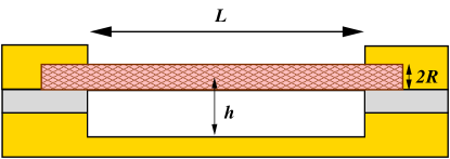
Figure 1: Illustration of suspended nanotube device.

2 Electrostatics of charge nanotube

We now discuss the electrostatics of the charge suspended nanotube. First we consider the longitudinal electric field, and then the radial field.

2.1 Electric field parallel to the nanotube

For a metallic tube there would, of course, be no electric field in the longitudinal direction. However, the tube has a finite screening length due to the kinetic energy. We have analyzed this situation using the following density functional for the total energy of a nanotube with linear dispersion

$$F[\rho]=\frac{\hbar}{2}\int_{0}^{L}dx\,v_{\mathrm{F}}(x)[\rho(x)]^{2}+\frac{1}{2}\int_{0}^{L}dx\int_{0}^{L}dx^{\prime}\,\rho(x)V(x,x^{\prime})\rho(x^{\prime}),$$ (1)

where $v_{F}$ is the Fermi velocity and $V(x,x^{\prime})$ is the effective 1D potential for a cylindric conductor. Details about the interaction and the solution are given in Appendix A. One should include screening due to both gate and source-drain electrodes. The gate can be included as a metallic plane at some distance $h$, and the source-drain electrodes as a section of the wire with $v_{\mathrm{F}}=0$. See figure 2 for an illustration of this.

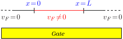
Figure 2: The model used to find the electric. The electrodes are represented by a 1D lead with $v_{F}=0$.

To minimize the energy functional in equation (1) under the constraint that a charge of one electron is added to the tube, we add a Lagrange multiplier

$$F_{1}[\rho,\lambda]=E[\rho]+\lambda\left(\int_{0}^{L}dx\rho(x)-e\right).$$ (2)

First, we minimize with respect to $\rho$ and find

$$\frac{\delta F_{1}}{\delta\rho[x]}=\hbar v_{\mathrm{F}}\rho(x)+\int_{0}^{L}dx^{\prime}\,V(x,x^{\prime})\rho(x^{\prime})+\lambda=0,$$ (3)

and then with respect to $\lambda$:

$$\frac{\partial F_{1}}{\partial\lambda}=\int_{0}^{L}dx\rho(x)-e=0.$$ (4)

These two linear equations are readily solved numerically. Once the solution is found, the electric field is given by

$$eE_{x}(x)=-\frac{\partial}{\partial x}\int_{0}^{L}dx^{\prime}\,V(x,x^{\prime})\rho(x^{\prime}).$$ (5)

The important parameters in this solution are the aspect ratio of the tube, i.e., $\frac{L}{R}$, and the strength of the interaction

$$r=\frac{e^{2}}{4\pi\epsilon_{0}\hbar v_{\mathrm{F}}}.$$ (6)

For typical parameters, one has $r=10-20$, while the aspect ratio is $200-2000$. The distance to the gate is not important, as long as it longer than the length over which the electric decays, which is typically the case. Our numerical solution gives an electric field comparable to the results of Guinea[16] (see also reference [17]), which results in an electric force of order $eE_{x}\sim 10^{-9}$ N, for typical nanotube devices. However, this field is limited to a small region near the contacts, and therefore the total effect of it is small.

For $r\gg 1$, we can in fact make a simple approximation which quit accurately describes the full numerical solution. The electric field can related to the charge density by differentiating the condition (3) with respect to $x$:

$$eE_{x}(x)=\hbar\frac{\partial}{\partial x}\left[\rho(x)v_{F}(x)\right].$$ (7)

Because $\rho(x)$ changes little along the wire, we may set $\rho\approx 1/L$ and we thus obtain

$$eE_{x}(x)\approx\frac{\hbar v_{F}}{L}\left[\delta(x)-\delta(x-L)\right].$$ (8)

The width of the delta function will be given by microscopic details of the interface between the tube and the contact, i.e. a length scale of the order of the radius of the tube itself. This length scale we denote by $x_{0}$.

2.1.1 The electrostatic force in the longitudinal direction

The term in the Hamiltonian describing the interaction between the electron charge density and the nuclear system is

$$H_{\mathrm{el-vib},x}=-\int dxdx^{\prime}\,\rho(x)V(x,x^{\prime})\rho_{n}(x^{\prime}),$$ (9)

where $\rho_{n}(x)$ is the density of the positive ions in the tube. The force per length acting on the mechanical degrees of freedom is therefore given by $eE_{x}\rho_{n}$. In terms of the displacement field defined below in equation (18), $H_{\mathrm{el-vib},x}$ becomes

$$H_{\mathrm{el-vib},x}=-\rho_{0}\int dx\,\rho(x)V(x,x^{\prime})\left[\partial_{x^{\prime}}u(x^{\prime})\right]=-e\rho_{0}\int dx\,E_{x}(x)\,u(x).$$ (10)

2.2 Electric field perpendicular to the nanotube

To find the electric field in the radial direction we model the nanotube as a distributed capacitor similarly to Sapmaz et al.[18]. We include capacitances to the electrodes $C_{l}$ and to the gate

$$C=C_{l}+C_{g},$$ (11)

where the capacitance to the gate is

$$C_{g}=\int_{0}^{L}dx\,c(h(x)),\quad c(h)=\frac{2\pi\epsilon_{0}}{\cosh^{-1}(h/R)},$$ (12)

with $c$ being the distributed capacitance of a tube over a plane.

To find the total charge on the tube, we write the total electrostatic energy as

$$W=\frac{q^{2}}{2C}-q\Delta\Phi/e,$$ (13)

where $C$ is total capacitance with charge $q$ and $\Delta\Phi$ is the difference between the nanotube and the electrode work functions. (Here we neglect the effect of the source, drain and gate voltages, because they are considerably smaller than $\Delta\phi$.) The optimum charge is thus

$$q_{0}\equiv n_{0}e=\Delta\Phi\,C/e.$$ (14)

For single-walled carbon nanotubes the workfunction is about 4.7 eV[19, 20, 21], while for gold it is 5.1 eV. For typical devices $C\sim 10^{-17}$ F and hence $n_{0}\sim 30$. The electrostatic energy is used in the following section to calculate force acting on the tube.

2.2.1 The electrostatic force in the transverse direction

Below we solve for the distortions of the wire due to the electrostatic forces. The force in the direction perpendicular to the charged wire (denoted the $z$-direction) is given by

$$k=-\frac{dW}{dC_{g}}\left.\frac{\delta c_{g}}{\delta z(x)}\right|_{z=0}=\,\left(\frac{C_{g}}{C}\right)^{2}\frac{e^{2}n_{0}^{2}}{4\pi\epsilon_{0}hL^{2}},$$ (15)

where

$$\left.\frac{\delta c_{g}}{\delta z(x)}\right|_{z=0}=\frac{2\pi\varepsilon_{0}}{h\left[\cosh^{-1}(h/R)\right]^{2}}=\frac{C_{g}^{2}}{2\pi\epsilon_{0}hL^{2}},\quad\mathrm{with}\,C_{g}=Lc(0).$$ (16)

3 Elastic properties

In this section, we discuss in detail the elastic properties of a suspended nanotube. Most devices are made by under-etching after depositum of the nanotube, which is done at room temperatures. Therefore, since the thermal expansion coefficient of nanotubes is negative (100 nm wire expands a few nm from room temperature to 4 K) it seems unlikely that there is a large tension in tube unless it becomes heavily charged[18]. When the tube is charged it is attracted towards the metallic gates and leads.

The radial force, off course, couples to the breathing-type modes, which, however, have too large energies ($\sim$ 30 meV) to be relevant for the low-voltage experiment in reference [3]. Here we are interested in the lower part of the excitation spectrum and disregard this mode. We are left with the bending and stretching modes. The energy of the bending is typically much lower than those of stretching modes[7], and therefore we treat these as purely classical, which means that we will solve for the bending mode separately and then via an anharmonic term this solution acts as a force term on the longitudinal mode.

We thus consider two possible mechanism for coupling to the stretching mode: either directly via the longitudinal electric field discussed in section 2.1 or through the perpendicular field, section 2.2, which bends the tubes and hence also stretches it.

3.1 Elasticity theory of a hanging string

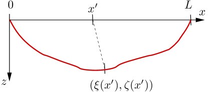
Figure 3: The coordinate system used to describe the hanging tube. A point on the tube, which before the distortion was at $(x^{\prime},0)$ has after the deformation the coordinates $(\xi(x^{\prime}),z(x^{\prime})).$

Assuming the tube to lie in a single plane and thus having no torsion in the longitudinal direction, we can describe the distortion of the bend tube by $(\xi(x),z(x))$, where $x\in[0,L]$ runs along the unbend tube in absence of external forces, see figure 3. (If the tube has some slack, $x$ is a curve linear coordinate along the equilibrium position the hanging tube.) This means that a point along the tube, which before was at $(x,0)$ after the deformation has the coordinates $(\xi(x),z(x)).$ The total elastic energy of the tube is then follows from standard elasticity theory of an elastic string[22]

$$W=\int_{0}^{L}dx\left(\frac{EA[\zeta(x)]^{2}}{2}+\frac{EI}{2[R(x)]^{2}}+k_{\perp}z(x)+k_{\parallel}\;u(x)\right),$$ (17)

where $\zeta$ is the linear strain of extension, $R$ is the radius of curvature, $A=\pi R^{2}$ the area and $I=\pi R^{4}/4$ the moment of inertia, $E$ is Young’s modulus, and $k_{\parallel},k_{\perp}$ the external forces, and where we have defined the longitudinal displacement field as

$$u(x)=\xi(x)-x.$$ (18)

The linear extension of an infinitesimal element between $x$ and $x+dx$ is

$$\zeta(x)dx=\sqrt{(\xi(x+dx)-\xi(x))^{2}+(z(x+dx)-z(x))^{2}}-dx,$$ (19)

or

$$\zeta(x)=\left(\sqrt{[1+u^{\prime}(x)]^{2}+[z^{\prime}(x)]^{2}}-1\right).$$ (20)

The linear extension elastic energy is thus

$$W_{\mathrm{lin}}=\frac{EA}{2}\int_{0}^{L}dx\left(\sqrt{[1+u^{\prime}(x)]^{2}+[z^{\prime}(x)]^{2}}-1\right)^{2}.$$ (21)

The curvature contribution is determined in a similar way. First, the unit tangential vector is

$$\mathbf{t=}\frac{\left(\xi^{\prime}(x),z^{\prime}(x)\right)}{\sqrt{[\xi^{\prime}(x)]^{2}+[z^{\prime}(x)]^{2}}},$$ (22)

which then gives the square of the radius of curvature as

$$R^{-2}=\left(\frac{d\mathbf{t}}{dl}\right)^{2}=\left(\frac{d\mathbf{t}}{dx}\frac{dx}{dl}\right)^{2},\quad\frac{dl}{dx}=\sqrt{[1+u^{\prime}(x)]^{2}+[z^{\prime}(x)]^{2}},$$ (23)

and then the curvature contribution to the elastic energy finally becomes

$$W_{\mathrm{curv}}=\frac{EI}{2}\int_{0}^{L}dx\,\frac{(z^{\prime}(x)u^{\prime\prime}(x)-(1+u^{\prime}(x))z^{\prime\prime}(x))^{2}}{([1+u^{\prime}(x)]^{2}+[z^{\prime}(x)]^{2})^{3}}.$$ (24)

3.2 Weak distortions

Since we are interested in small deflections, we expand the two elastic energy expressions for small $z$ and $u.$ For $W_{\mathrm{lin}}$, we obtain to third order in $u$ and $z$

$$W_{\mathrm{lin}}\approx\frac{EA}{2}\int_{0}^{L}\,dx\left([u^{\prime}(x)]^{2}+\frac{[z^{\prime}(x)]^{4}}{4}+u^{\prime}(x)[z^{\prime}(x)]^{2}\right).$$ (25)

Here we note that the last term couples the bending and stretching modes. For the curvature contribution, we find to the same order

$$W_{\mathrm{cur}}=\frac{EI}{2}\int_{0}^{L}dx\,\left(1-4u^{\prime}(x)\right)\left[z^{\prime\prime}(x)\right]^{2}\approx\frac{EI}{2}\int_{0}^{L}dx\,\left[z^{\prime\prime}(x)\right]^{2}.$$ (26)

Again, there is a term which couples the two modes. However, for nanotubes this term is much smaller than the last term in equation (25), because it smaller by a factor $(R/L)^{2}$, and hence we have neglected the coupling term in $W_{\mathrm{cur}}$.

4 Solution for the bending of the tube

As mentioned above, the bending mode itself has a resonance frequency too low to be seen tunnelling spectroscopy ($\sim 100$ MHz[7])(even when under tension due to the charging of the wire ), which means that it can be treated as a classical degree of freedom and Franck-Condon type physics is not involved. In contrast, the longitudinal stretching mode has been seen in the single-electron-transistor (SET) device[3] and here we wish to calculate the Franck-Condon coupling constants for this mode. Therefore we take the following approach: first we solve for the bending mode classically and then insert this as an external force acting on the longitudinal mode. The differential equation for $z(x)$ is

$$IEz^{\prime\prime\prime\prime}-\frac{AE}{2}(z^{\prime})^{2}z^{\prime\prime}=k.$$ (27)

This equation cannot be solved analytically. One approach is to approximate $(z^{\prime})^{2}$ by the average value, which is corresponds to assuming constant tension in the wire[23].

Below we solve for the bending function $z(x)$ in two regimes: the linear and the non-linear regime. Once we know $z(x)$, we will be interested in the change of $z(x)$ due to tunnelling of a single electron. For large $n_{0}$, the relevant change is thus

$$z_{e}(x)=\frac{dz(x)}{dn_{0}}.$$ (28)

This change will then couple to the longitudinal mode via the coupling term in equation (25).

4.1 Linear regime

For weak forces we can simply neglect the non-linear term in equation (27), and with boundary conditions $z(0)=z(L)=z^{\prime}(0)=z^{\prime}(L)=0$ the solution is

$$z_{0}(x)=\frac{kL^{4}}{24EI}\left(1-\frac{x}{L}\right)^{2}\left(\frac{x}{L}\right)^{2}.$$ (29)

The shift in $z_{0}(x)$ due to the charge of a single electron is according to equation (28) given by

$$z_{0,e}(x)=\frac{e^{2}n_{0}}{12\pi\epsilon_{0}h}\frac{1}{EA}\left(\frac{L}{R}\right)^{2}\left(\frac{C_{g}}{C}\right)^{2}\left(1-\frac{x}{L}\right)^{2}\left(\frac{x}{L}\right)^{2}.$$ (30)

For a tube with $R=$ 0.6 nm, $L=1\,\mu$m, and $E\approx 10^{12}$ Pa and a device with $h=200$ nm, $n_{0}=50$, and $C_{g}/C=0.5$, the maximum distortion is of order a few nm.

The linear approximation is valid when the second term in equation (27) is much smaller than the first. Using the solution in equation (29), this translates to the condition

$$10^{-6}\left(\frac{L}{R}\right)^{2}\left(\frac{kL^{3}}{EI}\right)^{2}\ll 1.$$ (31)

For the typical parameters used below, the number on the left hand side of (31) is $\lesssim 1$, and therefore the linear approximation is only marginally valid.

4.2 Non-linear regime.

For larger distortions the non-linear term in equation (27) becomes important. In the strongly non-linear regime, we can neglect the first term and we have

$$\frac{AE}{2}(z^{\prime})^{2}z^{\prime\prime}=\frac{AE}{6}\frac{d}{dx}(z^{\prime})^{3}=-k,$$ (32)

with boundary condition $z(0)=z(L)=0$. The solution of this equation is

$$z_{1}^{\prime}(x)=\left(\frac{6kL^{3}}{EA}\right)^{1/3}\left|\frac{x}{L}-\frac{1}{2}\right|^{1/3}\mathrm{sign}\left(\frac{L}{2}-x\right).$$ (33)

In this non-linear regime, the change in the slope the bending function $z_{1}(x)$ due to a single electron charge, is

$$z_{1,e}^{\prime}(x)=2\left(\frac{C_{g}}{C}\right)^{2/3}\left(\frac{e^{2}}{2\pi\epsilon_{0}hAn_{0}}\right)^{1/3}\left|\frac{x}{L}-\frac{1}{2}\right|^{1/3}\mathrm{sign}\left(\frac{L}{2}-x\right).$$ (34)

5 Distortion of the longitudinal mode

Due to the electrostatic forces the equilibrium position of longitudinal displacement field $u(x)$ shifts. Since the forces are small the displacement is going to be small. For the tunnelling overlap factors, the important point is, however, whether these displacements are large compared to the quantum uncertainty length, which later is seen to be of order of pm. In this section, we calculate the classical displacements of $u(x)$. One example is shown in figure 4.

5.1 Distortion due to the longitudinal electrostatic force

The displacement of the longitudinal mode is readily found from its equation of motion. The displacement due to the longitudinal electric field follows from

$$EAu^{\prime\prime}_{0}(x)=k_{\parallel}(x)=-eE_{x}\rho_{0},$$ (35)

with boundary conditions $u(0)=u(L)=0$. With forces concentrated near the contacts as in equation (8), there is an abrupt change of $u(x)$ at $x=0$ and $x=L$. See figure 2 red dashed curve.

5.2 Distortion due to the transverse electrostatic force

Once we have solved for $z(x)$ in equation (28), we can find the force that acts on the longitudinal diplacement field $u$ by inserting the solution into the last term of equation (25), and then identify the force $k_{\perp}$ in equation (17). This gives

$$k_{\perp}=\frac{d}{dx}\frac{EA}{2}[z^{\prime}(x)]^{2}.$$ (36)

The size of the displacement follows from the balance between this force and the strain:

$$EAu^{\prime\prime}_{0}(x)=k_{\perp}(x)\Leftrightarrow u^{\prime\prime}_{0}(x)=z^{\prime}(x)z^{\prime\prime}(x),$$ (37)

which together with the boundary condition, $u_{0}(0)=u_{0}(L)=0$, gives the solution

$$u_{0}(x)=-\frac{1}{2}\int_{0}^{x}dy\,[z^{\prime}(y)]^{2}+\frac{x}{2L}\int_{0}^{L}dy\,[z^{\prime}(y)]^{2}.$$ (38)

One example is shown in figure 2 (blue curve).

In the next section, we analyze the Franck-Condon overlap factor due to this electrostatic distortion of the stretching mode.

Figure 4: The solutions for the shifted longitudinal mode $u(x)$ due to the parallel (red dashed curve) and perpendicular (blue curve) electric fields. We have used typical parameters as in section 6.3

6 Quantum mechanics and Franck-Condon overlap factors

The longitudinal eigenmodes of a nanotube modeled as a 1D elastic medium follows from the Hamiltonian

$$\hat{H}=\int_{0}^{L}dx\left(\frac{\hat{p}^{2}(x)}{2\rho_{m}}+\frac{AE}{2}(\partial_{x}\hat{u}(x))^{2}\right),$$ (39)

where $\rho_{m}$ is mass density per unit length, and $\hat{u}$ and $\hat{p}$ are conjugated variables, i.e., $[\hat{u}(x),\hat{p}(x^{\prime})]=i\hbar\delta(x-x^{\prime})$. In order to diagonalize $\hat{H}$, we introduce the Fourier transforms:

$$\hat{u}(x) = \sqrt{2}\sum_{n=1}^{\infty}\sin\left(\frac{\pi nx}{L}\right)\hat{u}_{n},\quad\hat{u}_{n}=\frac{\sqrt{2}}{L}\int_{0}^{L}dz\sin\left(\frac{\pi nx}{L}\right)\hat{u}(x),$$ (40)

$$\hat{p}(x) = \frac{\sqrt{2}}{L}\sum_{n=1}^{\infty}\sin\left(\frac{\pi nx}{L}\right)\hat{p}_{n},\quad\hat{p}_{n}=\sqrt{2}\int_{0}^{L}dz\sin\left(\frac{\pi nx}{L}\right)\hat{p}(x),$$ (41)

where $\hat{u}_{n}$ and $\hat{p}_{n}$ obey $[\hat{u}_{n},\hat{p}_{n}]=i\hbar$. Now $\hat{H}$ transforms to

$$\hat{H}=\sum_{n=1}^{\infty}\left(\frac{\hat{p}_{n}^{2}}{2M}+\frac{AE}{2L}\left(\pi n\right)^{2}\hat{u}_{n}^{2}\right),\quad M=\rho_{m}L,$$ (42)

The Hamiltonian (42) is easily diagonalized by

$$\hat{u}_{n}=\ell_{0,n}\sqrt{\frac{1}{2}}\left(\hat{a}_{n}+\hat{a}_{n}^{\dagger}\right),\quad\hat{p}_{n}=\frac{i}{\ell_{0,n}}\sqrt{\frac{1}{2}}\left(\hat{a}_{n}^{\dagger}-\hat{a}_{n}\right),$$ (43)

where $\hat{a}_{n}$ and $\hat{a}_{n}^{\dagger}$ are usual annihilation and creation operators, and

$$\Omega=\pi\sqrt{\frac{AE}{ML}}=\frac{\pi}{L}\sqrt{\frac{AE}{\rho_{m}}}\equiv\frac{\pi v_{s}}{L},\quad\ell_{0,n}=\sqrt{\frac{\hbar}{nM\Omega}}.$$ (44)

With these operators, the Hamiltonian (42) becomes

$$\hat{H}=\sum_{n=1}^{\infty}\hbar\Omega n\left(\hat{a}_{n}^{\dagger}\hat{a}_{n}+\frac{1}{2}\right).$$ (45)

As we saw in the previous sections, additional terms in the Hamiltonian appears due to the force generated by the tunnelling electron. These are included next.

6.1 Coupling due to longitudinal electric field

The longitudinal electric field $E_{x}$ gives rise to a coupling Hamiltonian (see equation (10)):

$$\hat{H}_{\mathrm{el-vib},\parallel}=-e\rho_{0}\int_{0}^{L}dx~{}\hat{u}(x)E_{x}(x)=\sum_{n=1}^{\infty}\hat{u}_{n}f_{n,\parallel},$$ (46)

where

$$f_{n,\parallel}=-e\rho_{0}\sqrt{2}\int_{0}^{L}dx~{}\sin\left(\frac{\pi nx}{L}\right)E_{x}(x)\approx-(2\pi\sqrt{2})\frac{n\hbar v_{\mathrm{F}}\rho_{0}x_{0}}{L^{2}},$$ (47)

for $n$ even and zero for $n$ odd.

6.2 Coupling due to the capacitative force

The transverse force leads to the following term in the Hamiltonian (see equation (25)):

$$\hat{H}_{\mathrm{el-vib},\perp}=\frac{EA}{2}\int_{0}^{L}dx~{}\hat{u}^{\prime}(x)[z^{\prime}_{e}(x)]^{2}=\sum_{n=1}^{\infty}\hat{u}_{n}f_{n,\perp}.$$ (48)

where

$$f_{n,\perp}=\frac{EA}{\sqrt{2}}\frac{n\pi}{L}\int_{0}^{L}dx~{}\cos\left(\frac{\pi nx}{L}\right)[z^{\prime}_{e}(x)]^{2}.$$ (49)

6.3 Franck-Condon overlap factors

The tunnelling of an electron leads to a displacement of the equilibrium displacement field according to equations (46),(48). Each mode represented by $\hat{u}_{n}$ is shifted by the amounts

$$\ell_{n,a}=\frac{Lf_{n,a}}{AE(\pi n)^{2}},\quad a=(\parallel,\perp).$$ (50)

This allows us to calculate the Franck-Condon parameters, which for each mode $n$ expresses the overlaps between the new eigenstates around the new equilibrium positions and the old one. This parameter is defined as[14]

$$g_{n,a}=\frac{1}{2}\left(\frac{\ell_{n,a}}{\ell_{0,n}}\right)^{2}.$$ (51)

The size of $g$ determines the character of the vibron sidebands in the $IV$-characteristics, such that for $g\ll 1$ there are no sidebands, for $g$ of order one clear sidebands are seen, while for $g\gg 1$ a gap appears in $IV$ characteristic[14, 15].

For the Franck-Condon parameter due to the parallel electric field, we thus have

$$g_{n,\parallel}=\frac{4}{\pi^{2}n^{2}}\,\frac{M\Omega}{\hbar}\left(\frac{\hbar v_{\mathrm{F}}\rho_{0}x_{0}}{AEL}\right)^{2}.$$ (52)

Using $x_{0}\approx 1$ nm, $L=500$ nm, $v_{\mathrm{F}}=10^{6}$ ms^-1, $R=0.6$ nm, and $E=10^{12}$ Pa, we find $g_{2,\parallel}\sim 10^{-5}$. This is clearly too small a coupling constant to explain the experimental findings in reference [3].

The coupling constant due to the perpendicular electric can be expressed explicitly, for the case of small $z(x)$, using equation (29). The integral in equation (49) can then be performed and we obtain

$$g_{n,\perp}=\frac{M\Omega L^{2}}{\hbar}\left(\frac{k_{e}L^{3}}{EI}\right)^{4}\frac{\left(n^{2}\pi^{2}-40\right)^{2}}{8n^{13}\pi^{14}},\quad\mathrm{for}\quad n\quad\mathrm{even},$$ (53)

and zero for $n$ odd. Using $k_{e}$ as defined in equation (15), and typical parameter for single wall carbon nanotube devices: $R=0.6$ nm, $L=1\,\mu$m, $E=10^{12}$ Pa, $h\simeq 10-200$ nm, $n_{0}=Lc(0)\Delta\phi\sim 30$, $C_{g}/C=0.1-0.75$, we find the maximum $g_{n}$ factor to occur for $n=4$. However, for this range of parameters we also find $g_{4}\ll 1$, unless the geometry is such that

$$\frac{n_{0}\alpha^{2}}{h[\mathrm{nm}]}>0.1.$$ (54)

Even though we can get a significant coupling, the condition (54) does not seem to be compatible with the experimental realizations in reference [3]. Even more so because the coupling strongly strength, equation (53), depends strongly on the length of wire, which is not seen experimentally.

7 Conclusion and discussion

We have considered the electromechanics of suspended nanotube single-electron-transistor devices. When the charge on the tube is changed by one electron the resulting electric field will distort the tube in both the longitudinal and transverse directions, and both these distortions couple to the stretching mode. We have calculated they consequences for the coupling constant for vibron-assisted tunnelling expressed as the Franck-Condon factor. This is expressed in terms of the ratio of the classical displacement to the quantum uncertainty length. Even though both are in the range of picometers, the effective coupling parameters, $g$, turn out to be small for most devices.

Because the screening of the longitudinal electric field is very effective, the dominant interaction seems to be the coupling via the bending mode. However, only if the tube is very close to the gate do we get a sizeable $g$-parameter. This could indicate that in the experiment of Sapmaz et al.[3] the suspended nanotube has a considerable slack, which would diminish the distance to the gate. Further experiments and more precise modelling of actual geometries should be able to resolve these issues.

Appendix A Electric field in a charged nanowire

A.1 The effective 1D interaction

Here we derive in more detail the result show in section 2. The interaction between two charges on points $x$ and $x^{\prime}$ is

$$V(x-x^{\prime})=\int d\mathbf{r}_{\perp}\int d\mathbf{r}_{\perp}^{\prime}\frac{e^{2}|\phi({r}_{\perp})|^{2}|\phi({r}_{\perp}^{\prime})|^{2}}{4\pi\epsilon_{0}\sqrt{(x-x^{\prime})^{2}+(\mathbf{r}_{\perp}-\mathbf{r}_{\perp}^{\prime})^{2}}},$$ (55)

where $\phi(\mathbf{r}_{\perp})$ is the wavefunction is the perpendicular direction. By modelling the tube as a cylinder, $\phi(\mathbf{r}_{\perp})=\delta(r-R)/2\pi R$, we get

$$V(x-x^{\prime}) = \frac{e^{2}}{2\pi\epsilon_{0}}\int_{0}^{2\pi}\frac{d\theta}{\sqrt{(x-x^{\prime})^{2}+(2R\sin(\theta/2)^{2}}}$$ (56)

$$= \frac{2e^{2}}{2\pi^{2}\epsilon_{0}\sqrt{(x-x)^{2}+4R^{2}}}\,K\!\left(\frac{4R^{2}}{(x-x^{\prime})^{2}+4R^{2}}\right),$$

where $K$ is the complete elliptic integral of the first kind. With screening due to a gate at distance $h\gg R$, the interaction is

$$V_{\mathrm{scr}}(x-x^{\prime})=V(x-x^{\prime})-\frac{e^{2}}{4\pi\epsilon_{0}\sqrt{(x-x^{\prime})^{2}+(2h)^{2}}}.$$ (57)

References

- [1] J. Nygård and D. Cobden, App. Phys. Lett. 79, 4216 (2001).
- [2] B. LeRoy et al., Phys. Rev. B 72, 075413 (2005).
- [3] S. Sapmaz et al., cond-mat/0508270.
- [4] J. M. Kinaret, T. Nord, and S. Viefers, App. Phys. Lett. 82, 1287 (2003).
- [5] L.M. Jonsson et al., Nanotechnology 15, 1497 (2004).
- [6] L.M. Jonsson, L.Y. Gorelik, R.I. Shekhter, and M. Jonson, Nano Lett. 5, 1165 (2005).
- [7] H. Üstünela, D. Roundy, and T. Arias, Nano Lett. 5, 523 (2005).
- [8] W. Izumida and M. Grifoni, cond-mat/0509597.
- [9] H. Suzuura and T. Ando, Phys. Rev. B 65, 235412 (2002).
- [10] H. Park et al., Nature 407, 57 (2000).
- [11] A. N. Pasupathy et al., Nano Lett. 5, 203 (2005).
- [12] D. Boese and H. Schoeller, Europhys. Lett. 54, 668 (2001).
- [13] K. McCarthy, N. Prokof’ev, and M. Tuominen, Phys. Rev. B 67, 245415 (2003).
- [14] S. Braig and K. Flensberg, Phys. Rev. B 68, 205324 (2003).
- [15] J. Koch, M.E. Raikh, and F. von Oppen, Phys. Rev. Lett. 95, 056801 (2003).
- [16] F. Guinea, Phys. Rev. Lett. 94, 116804 (2005).
- [17] E.G. Mishchenko and M.E. Raikh, cond-mat/0507115.
- [18] S. Sapmaz, Y. M. Blanter, L. Gurevich, and H. S. J. van der Zant, Phys. Rev. B 67, 235414 (2003).
- [19] R. Gao, Z. Pan, and Z. Wang, App. Phys. Lett. 78, 1757 (2001).
- [20] J. Zhao, J. Han, and J. Lu, Phys. Rev. B 65, 193401 (2002).
- [21] B. Shan and K. Cho, Phys. Rev. Lett. 94, 23602 (2005).
- [22] L. D. Landau and E. M. Lifshitz, Theory of elasticity (Butterworth-Heinemann, Oxford, 1986).
- [23] The constant tension approximation is ony valid for forces concentrated to points[22], which is not the case here where the force is distributed. This is in constrast to the assumptions made in [18].