Monte Carlo simulation of an strongly coupled XY model in three dimensions

Abstract

Many experimental studies, over the past two decades, have constantly reported a novel critical behavior for the transition from Smectic-A phase of liquid crystals to Hexatic-B phase with non-XY critical exponents. However according to symmetry arguments this transition must belong to XY universality class. Using an optimized Monte Carlo simulation technique based on multi-histogram method, we have investigated phase diagram of a coupled XY model, proposed by Bruinsma and Aeppli (PRL 48, 1625 (1982)), in three dimensions. The simulation results demonstrate the existence of a tricritical point for this model, in which two different orderings are established simultaneously. This result verifies the accepted idea the large specific heat anomaly exponent observed for SmA-HexB transition could be due to the occurrence of this transition in the vicinity of a tricritical point.
PACS numbers: 71.30.+h, 71.23.An, 71.55.Jv

I Introduction

According to Kosterlitz, Thouless, Halperin, Nelson and Young (KTHNY) theory [1],[2],[3], two dimensional systems during melting transition from solid to isotropic liquid go through an intermediate phase called hexatic phase for systems that have six-fold(hexagonal) symmetry in their crystalline ground state. This hexatic phase displays short range positional order, but quasi long range bond-orientational order, which is different from the true long range bond-orientational and quasi long range positional order in 2D solid phases. It is known that for two dimensional systems, the transition from the isotropic liquid to hexatic phase could be either a KT transition or a first order transition [4].

The idea of hexatic phase was first applied to three dimensional systems by Birgeneau and Lister, who showed that some experimentally observed smectic liquid crystal phases ,consisting of stacked 2D layers, could be physical realization of 3D hexatics[5]. Assuming that the weak interaction between smectic layers could make the quasi long range order of two dimensional layers truly long ranged, they suggest that the 3D hexatic phases in highly anisotopic systems, possess short range positional and true long range bond-orientational order.

The first signs for the existence of the hexatic phase in three dimensional systems were observed in x-ray diffraction study of liquid crystal compound 65OBC(n-alkyl-4-m-alkoxybiphenyl-4-carboxylate,n=6,m=5)[6, 7], where a hexagonal pattern of diffuse spots was found in intensity of scattered x-rays. In addition to this hexagonal pattern, it was also found that some broader peaks were appeared in the diffracted intensity which indicate the onset of another ordering. These broad peaks are related to packing of molecules according to the herringbone structure perpendicular to the smectic layer stacking direction. The accompanying of the long range hexatic and short range herringbone orders make this phase a physically rich phase which simply is called Hexatic-B (HexB) phase. When temperature is decreased, the HexB phase transforms via a first order phase transition into the crystal-E (CryE) phase, which exhibits both long range positional and long range herringbone orientational orders. Subsequently, it was found that other components in nmOBC homologous series (like 37OBC and 75OBC) and a number of binary mixtures of n-alkyl-4’-n-decycloxybiphenyl-4-carboxilate (n(10)OBC) with n ranging from 1 to 3 and also the compound 4-propionyl-4’-n-heptanoyloxyazo-benzene (PHOAB) represent smA-HexB transition, which for later the transition has found to be clearly first order.

Due to the sixfold symmetry of hexatic phase, the corresponding order parameter is defined by $\Psi_{6}=|\Psi_{6}|\exp(i6\psi_{6})$. The U(1) symmetry of the $\Psi_{6}$, implies that SmA-HexB transition be a member of XY universality class. However, heat capacity measurements on bulk samples of 65OBC [6, 8] and other calorimetric studies on many other components in the nmOBC homologous series [6, 9] have yielded very sharp specific heat anomalies near SmA-HexB transition with no detectable thermal hystersis and with very large value for the heat capacity critical exponent, $\alpha\approx 0.6$. These results indicate that this is a continues (second order) phase transition, but not belonging to The 3D XY universality class, for which the specific heat critical exponent is nearly zero ($\alpha\approx-0.007$[11]).On the other hand, the other static critical exponents determined from thermal conductivity ($\eta=-0.19$)and birefringence experiments ($\beta=0.19$) [6], all differ from the 3D XY values, indicating a novel phase transition with probably a new universality class.

It is also interesting to mention that the same heat capacity measurement studies of (truly two-dimensional) two-layer free standing films of different nmOBC compound result a second order SmA-HexB transition, described by the heat capacity exponent $\alpha\approx 0.3$[6, 10]. This is obviously in contrast with the usual broad and nonsingular specific heat hump of the KT transition in the 2D XY model, suggesting that SmA-HexB transition can not be described simply by a unique XY order parameter.

The unusual aspects of SmA-HexB transition in two and three dimensions, have attracted the interests of physicists in the past two decades. The first theoretical attack to this problem was done by Bruinsma and Aeppli[12] who formulated a Ginzburg-Landau theory that included both hexatic and herringbone order. Because of the broadness of x-ray diffracted peaks associated to herringbone order (which is the reason of being short rang), they considered an XY order parameter with two fold symmetry for herringbone ordering $(\Phi_{2}=|\Phi_{2}|\exp(i2\phi_{2}))$ and also based on symmetry arguments, they made a minimal coupling between the hexatic and herringbone order parameters as $V_{hex-her}=hRe(\Psi_{6}^{*}\Phi_{2}^{3})$. Microscopically, the origin of this coupling could be the anisotropy presented in liquid crystals molecular structures[13, 14].

In the mean field approach their results indicate that the SmA-HexB transition should be continuous. However one-loop renormalization calculations show that short range molecular herringbone correlations coupled to the hexatic ordering drive this transition first order, which becomes second order at a tricritical point[12]. Their result indicates the existence of two tricritical points, one for the transition between SmA phase ($\Psi=0,\Phi=0$) and the stacked hexatic phase ($\Psi\neq 0,\Phi=0$), and another for the transition between the SmA and the phase possessing both hexatic and herringbone order ($\Psi\neq 0,\Phi\neq 0$). Therefore, They concluded that the occurrence of phase transition near the tricritical points, with heat capacity exponent $\alpha=0.5$, would be a good explanation for large heat capacity exponents observed in the experiments. Recently, the RG calculation of BA model has been revised in [15] which resulted in finding another non-trivial fixed point missed in original work of Bruinsma and Aeppli. But it has been shown that this new fixed point is unstable in one loop level (order of $\epsilon$), which refuses this fixed point to represent a novel phase transition. Improvement of this calculation to two loop level (order of $\epsilon^{2}$), although make this new fixed point stable, but gives a small and negative value for the corresponding heat capacity anomaly exponent [16], which indicts that this critical point can not explain the experimental results. However, the limitations of RG methods which mostly rely on perturbation expansions, make them insufficient for accessing the strong coupling regimes where one expect that some kind of new treatment to appear. For this purpose, the numerical simulations would be useful.

The first numerical simulations for investigating the nature of the SmA-HexB transition in 2D systems have been done by Jiang et al who have used a model consists of a 2D lattice of coupled XY spins based on the BA Hamiltonian in strong coupling limit[17, 18]. Their simulation results suggest the existence of a new type phase transition in which two different orderings are simultaneously established through a continuous transition with heat capacity exponent $\alpha\sim 0.3$, in good agreement with experimental values.

The success of BA model in two dimensions and also the absence of any numerical simulation in three dimensions were our motivations to investigate numerically the 3-dimensional BA model in strong coupling limit .To do this, we employ a high resolution Monte Carlo simulation based on multi-histogram method.

The rest of this paper is organized as follows. In section. II, we introduce model Hamiltonian and give a brief introduction to optimized Monte Carlo method based on multiple histograms and also Some methods for analyzing the Monte Carlo data, to determine the order of transitions. The simulation results and discussion is given in section III and conclusions will appear in section IV.

II Monte Carlo simulation

A Model Hamiltonian

Recalling the six-fold symmetry of hexatic order and two-fold symmetry of the herringbone order, the Hamiltonian which describes both orderings ought to be invariant with respect to the transformation $\Phi\rightarrow\Phi+n\pi$ and $\Psi\rightarrow\Psi+m(2\pi/6)$ where $n$ and $m$ are integers. Thus to lowest order in $\Psi$ and $\Phi$, one can write the following Hamiltonian for BA model:

$$H= - J_{1}\sum_{<ij>}\cos(\Psi_{i}-\Psi_{j})-J_{2}\sum_{<ij>}\cos(\Phi_{i}-\Phi_{j})$$ (1)

$$- J_{3}\sum_{i}\cos(\Psi_{i}-3\Phi_{i}),$$ (2)

where the coefficients $J_{1}$ and $J_{2}$ are the nearest-neighbor coupling constants for the bond-orientational order $(\Psi)$ and herringbone order $(\Phi)$, respectively. The coefficient $J_{3}$ denotes the coupling strength between these two types of order at the same 3D lattice site. we are interested in situations in which $\Psi$ and $\Phi$ are coupled strongly. Therefore we fixed $J_{3}=3.0$,larger that both $J_{1}$ and $J_{2}$ for all the simulations. Let assume $J_{1}>J_{2}$, so for sufficiently high temperatures,(say $T>J_{3}$), the system is in completely disordered phase. For $T_{c1}<T<J_{3}$, the system remains disordered but the phases of the two order parameters become coupled through the herringbone-hexatic coupling term $J_{3}$. In mean field level, for $T_{c2}<T<T_{c1}$, bond orientational order is established through a continuous XY transition and the ordered state corresponds to $\Psi_{i}\approx\Psi_{j}$ for all sites i and j, producing three degenerate minima for the free energy. So for these range of temperatures the BA Hamiltonian describes a system with the symmetry of the three-state potts model and since the ordering transition for three-state potts model is first order in 3D, the transition between the pure hexatic and hexatic plus herringbone phases ($\Psi\neq 0,\Phi\neq 0$) should be first order at $T_{c2}$. Thus for $J_{2}<J_{1}<J_{3}$ the model exhibits an XY transition at $T_{c1}$ and a three-state potts-like transition upon decreasing the temperature down to $T_{c2}$[19]. For $J_{2}>J_{1}$, the herringbone order would establish first and cause the correspondent field $\Phi$ to take nearly the same value for all sites. Because of this, the coupling term $J_{3}$ acts like a field on $\Psi$ and so the hexatic order parameter takes a nonzero value.

The above discussions results that the phase diagram of the BA model, in mean field level, consists of three phase transition: 1)A second order Transition from disordered to hexatic phase, 2)A second order transition from disordered to locked phase consist of hexatic plus herringbone orders and 3)A first order transition from hexatic to hexatic plus herringbone phases.

To obtain a qualitative picture of transitions and also the approximate location of the critical points, we first set a low resolution simulations. The Simulations were carried out using standard Metropolis spin-flipping algorithm with six lattice sizes (L=6,7,8,,9,10,12). During each simulation step, The angles $\Psi_{i}$ and $\Phi_{i}$ were treated as unconstrained, continuous variables. The random-angles rotations ($\Delta\Psi_{i}$ and $\Delta\Phi_{i}$) were adjusted in such a way that roughly $50\%$ of the attempted angle rotations were accepted. To ensure thermal equilibrium, 100 000 Monte Carlo steps (MCS) per spin were used for each temperature and 200 000 MCS were used for data collection.

We have obtained the heat-capacity data as a function of temperature, shown in Fig. (1) for $J_{1}=1.0$ and $J_{2}=0.5$ and for $J_{2}=0.7,0.8,0.9,1.2$ in Fig. (2). Near the lower temperature transition point ($1.2<T<1.35$) the calculated data were obtained by optimized reweighting using 5 histograms near $T=1.25$(section III). From the preceding discussion, it is clear that the small broad peak near T=2.2 signals the XY transition due to the $J_{1}$ term, while the sharp peak located at $T\sim 1.25$ is expected to signal a transition into the state of three-state potts symmetry. The same simulations based on single spin flipping algorithm whose results are represented in Fig.(2), show that the first peak (XY transition) would disappear for $J_{2}>0.9$ and therefore only one transition occurs for those values of $J_{2}$, which verifies that for these values of $J_{2}$, the transition from disordered to herringbone phase, simultaneously induces hexatic ordering .

To determine The location of the transition temperatures and other thermodynamic quantities such as specific heat near the transition points we need to use high resolution methods. For this purpose we used multiple-histogram reweighting method proposed by Ferrenberg and Swendsen [20], which makes it possible to obtain accurate data over the transition region from just a few Monte Carlo simulations.

B Histogram Method

The central idea behind the histogram method is to build up information on the energy probability density function $P_{\beta}(E)$, where $\beta=1/T$ is inverse temperature (in units with $k_{B}=1$). A histogram $H_{\beta}(E)$ which is the number of spin configurations generated between $E$ and $E+\delta E$. $P_{\beta}(E)$ is defined as :

$$P_{\beta}(E_{i})=\frac{H_{\beta}(E_{i})}{Z_{\beta}},$$ (3)

where

$$Z_{\beta}=\sum_{i}H_{\beta}(E_{i}).$$ (4)

On the other hand we now that $P_{\beta}(E_{i})$ is proportional to the Boltzmann weight $\exp(-\beta E_{i})$ as:

$$P_{\beta}(E_{i})=\frac{g(E_{i})\exp(-\beta E_{i})}{Z_{\beta}},$$ (5)

in which $g(E_{i})$ is the density of states with energy $E_{i}$ and is independent of temperature. By knowing the probability distributions in a specific temperature, we can derive the density of states and find the probability distribution of energy at any temperature $\beta^{{}^{\prime}}$ as follows:

$$P_{\beta^{{}^{\prime}}}(E_{i})=\frac{P_{\beta}(E_{i})\exp[(\beta-\beta^{{}^{\prime}})E_{i}]}{\sum_{j}P_{\beta}(E_{j})\exp[(\beta-\beta^{{}^{\prime}})E_{j}]}.$$ (6)

In principle, $P_{\beta}(E)$ only provides information on the energy distribution of nearby temperatures. This is because the counting statistics in the wings of the distribution $H_{\beta}(E)$, far from the average energy at temperature $T$, will be poor.

To improve the estimation for density of states, one can take data at more than one temperature and combine the resultant histograms so as to take the advantages of the regions where each provide the best estimate for the density of states. This method has been studied by Ferrenberg and Swendsen who presented an efficient way for combining the histograms [20]. Their approach relies on first determining the characteristic relaxation time $\tau_{j}$ for the $j$th simulation and using this to produce a weighting factor $g_{j}=1+2\tau_{j}$. The overall probability distribution at coupling $K=\beta J$ obtained from $n$ independent simulation, each with $N_{j}$ configurations, is then given by :

$$P_{K}(E)=\frac{[\sum_{j=1}^{n}g_{j}^{-1}H_{j}(E)]e^{-KE}}{\sum_{j=1}^{n}N_{j}g_{j}^{-1}e^{-K_{j}E-f_{j}}},$$ (7)

where $H_{j}(E)$ is the histogram for the $j$th simulation and the factors $f_{j}$ are chosen self-consistently using Eq.(7) and

$$e^{f_{j}}=\sum_{E}P_{K_{j}}(E).$$ (8)

Thermodynamic properties are determined, as before, using this probability distribution, but now the results would be valid over a much wider range of temperatures than for any single histogram. In addition, this method gives an expression for the statistical error of $P_{K}(E)$ as:

$$\delta P_{K}(E)=[\sum_{j=1}^{n}g_{j}^{-1}H_{j}(E)]^{-1/2}P_{K}(E),$$ (9)

from which it is clear that the statistical error will be reduced when more MC simulations are added to the analysis.

C Order of the transition

One of the main problems in Monte Carlo data analysis of phase transitions is determining the order of the transition. Strong first-order transitions will show marked discontinuities in thermodynamic quantities such as internal energy and the order parameter and present no real problems. Weakly first-order transition are much more difficult to recognize. To understand the situation, consider a first order phase transition in an infinitely extended system, for which the correlation length reaches a finite value $\xi_{c}$ at the transition point where the phase of the system changes discontinuesly. If $\xi_{c}$ is too large ,i.e $\xi_{c}>>L$ where $L$ is the linear size of the system on which the simulation is being done, then the system would appear to be in the critical region of a continues transition and it would be very difficult to detect the discontinuities. However, during the past decades, There have been significant advances in overcoming this problem. Below we list a number of techniques for detecting a first-order transition:
(1) Discontinuities in the internal energy and the order parameter.
(2) Hysteresis in the internal energy and the order parameter.
(3) Double peaks in the probability density function $P(E)$.
(4) The divergence of specific heat as $L^{d}$, where $d$ is the spatial dimension.
(5) Decreasing the Half-width of the specific heat peak like $L^{-d}$.
(6) The size dependence of the minima of Binder fourth energy cumulant

$$U_{4}(L)=1-\frac{<E^{4}>}{3<E^{2}>},$$ (10)

whose value approaches $2/3$ for a continuous transition and some nontrivial value $U^{*}<{2\over 3}$ at a first-order transition.

The first method as previously mentioned, is inefficient for weakly first order transitions. The second and third Methods are based on the fact that the state of a given system representing first order transition, during its evolution, may trap, for a relatively long time, in some local minima of free energy (called meta-stable states). these two methods are also unreliable because if the free-energy barrier is small enough, both phases will be sampled within time scale of the simulation, then no hysteresis will be observed. The second reason is that double peaks in the probability density function have also been observed near continuous transitions in finite systems, for examples in 4-states potts model in two dimensions. So the first three methods, although efficient for the case of strongly first order transitions, are nor suitable to investigate the weakly first order transitions. Methods (4) and (5) are the results of the discontinuity of internal energy at first-order phase transitions. Since the specific heat is obtained by derivative of internal energy respect to temperature, we expect that it present a delta function sigularity at the transition point. This causes the specific heat peak to diverge as $L^{d}$, while its half-width narrows like $L^{-d}$. Consequently, for the specific heat peak and transition temperature, we will have the following behaviours at a first order phase transition:

$$C_{max}(L)=c_{1}+c_{2}L^{d}$$ (11)

$$T_{c}(L)=T_{c}(\infty)+AL^{-d}.$$ (12)

The coefficient $c_{2}$ in eq.(11) is related to latent heat per site through the following relation:

$$c_{2}=\frac{(e_{1}-e_{2})^{2}}{4T_{c}^{2}},$$ (13)

where $e_{1}$ and $e_{2}$ are the values of energy per site at the transition point a first order phase transition. For a continuous phase transition, where the correlation length grows as $\xi\sim|T-T_{c}|^{-\nu}$ near a critical point, the behaviours of these two quantities are as :

$$C_{max}(L)=c_{1}+c_{2}L^{\frac{\alpha}{\nu}}$$ (14)

$$T_{c}(L)=T_{c}(\infty)+AL^{-\frac{1}{\nu}},$$ (15)

in which $\alpha$ is specific heat singularity exponent.

Method (6) is a test for the Gaussian nature of the probability density function $P(E)$ at $T_{c}$. For a continuous transition, $P(E)$ is expected to be Gaussian at, as well as away from $T_{c}$. For a first-order transition, $P(E)$ will be double peaked in infinite lattice size limit, hence deviation from being Gaussian cause the minimum of $U(L)$ tends $U^{*}$ to be less than $2/3$ as $L\rightarrow\infty$. $U^{*}$ is related indirectly to the latent heat. This is like the method (3) but much more sensitive, in a sense that small splitting in $P(E)$ for the infinite system that do not result in a double peak for small lattices can be detected. Another advantage of this technique is that the minimum of $U_{L}$ is expected to approach $2/3$ or $U^{*}$ as power law in $L$, thus allowing one to extrapolate to $L=\infty$ as:

$$U_{4}(L)|_{min}= \frac{2}{3}-\left(e_{1}/e_{2}-e_{2}/e_{1}\right)^{2}/12+BL^{-d}+$$ (17)

$$O(L^{-2d}),$$

The eq.(17) implies that:

$$U^{*}=\frac{2}{3}-\left(e_{1}/e_{2}-e_{2}/e_{1}\right)^{2}/12.$$ (18)

For weakly first order transitions where latent heat per site is too small ($\Delta e=e_{1}-e_{2}<<e_{1}$), we can write

$$U^{*}\approx\frac{2}{3}-(\Delta e/e)^{2}/3.$$ (19)

As an example we have used multi-histogram method (At least ten histograms were combined for each lattice size) to calculate the temperature dependent of $U_{4}(L)$ for $J_{1}=1.0$ , $J_{2}=0.8$ and $J_{3}=3.0$ depicted in Fig. (3), in which two minima exists for all values of linear lattice sizes ($L=6,7,8,9,10,12$). The right or high temperature minima indicate the transition from disorder to hexatic phase for which, we will show in what follows, that $U^{*}=2/3$, indicating a second order phase transition. The left or low temperature minima represent the transition from hexatic to hexatic plus herringbone phase. For this transition, however $U^{*}$ turns to be less than $2/3$ (table.I) showing that is a first order transition.

Since no hysteresis, discontinuities or double peaked $P(E)$ were observed in our simulation, we proceed to determine the order of the transition by scaling of the specific heat with lattice size and the determination of $U^{*}$ which is the most reliable method.

III results and discussion

In our work, at least five histograms were combined for each lattice size for different temperatures near $T_{c}$. For each histogram, we performed $5\times 10^{5}$ MCS for equilibration and $1\times 10^{6}$ for data collection, while 10 to 20 monte calro sweeps were discarded between successive measurements for decreasing the correlation between them. Because the energy spectrum is continuous, the data list obtained from a simulation is basically a histogram with one entry per energy value. In order to use the histogram method efficiently, we divide the energy range $E\leq 0$ into 20 000 and 200 000 bins and reconstructed the histograms. The results of the two binning agreed with each other within statistical errors. therefore we chose 20 000 bines throughout our simulation. In all simulations we fixed $J_{1}=1.0$ and $J_{3}=3.0$ and changed values of $J_{2}$ from 0.5 to 1.3.

Starting from $J_{2}=0.5$, for all lattice sizes, we observed two peaks in specific heat and two minima in the Binder forth energy cumulant vs temperatures in cooling run ( see Fig.(1) and Fig(3)). By increasing the value of $J_{2}$ those two peaks and minima get closer to each other as for $J_{2}=0.8$ the first peak change to be like a shoulder, while the two minima continue to be well separated. This behaviour can be traced until $J_{2}=0.9$ for which the two transitions merge to each other. For $J_{2}\geq 0.9$, also one peak and a minimum is obtained suggesting that $J_{2}=0.9$ can be considered as a critical end point in our simulation, above which only one transition from disordered to hexatic+herringbone phase would occur.

In what follows, we discuss separately the three transitions: 1)Isotropic-hexatic, 2)hexatic-hexatic+herringbone(locked phase) 3)Isotropic-hexatic+herringbone.

A Isotropic-hexatic transition

Using the Binder forth energy cumulant to determine the order of transition, we found that for all of those transitions for $J_{2}=0.5,0.6,0.7,0.8,0.85$, the minimum value of $U_{L}(U^{*})$ tends to $2/3$ within the statistical error of the simulation. For example in Fig.(4-a) we have ploted $U_{L}$ vs $L^{-3}$ for $J_{2}=0.7$. The best fitting of the data to eq.(17), by using least square procedure, shows that $U^{*}=0.66647(31)$ which is equal to $2/3$ within on e.s.d. This is true for all isotropic-hexatic transition points (table I). These results show that to the resolution of our simulation all of these transitions are second order.

To calculate the critical exponents we used the scaling relation of the maximum values of heat capacity per site ($C_{max}$) versus lattice sizes. The small range of the values of $C_{max}$ (i.e 2.54 for $L=6$ to 3.0 for $L=12$ for $J_{2}=0.7$ ) measured for all points along this critical line, is the characteristic of the transitions with cusp singularity in specific heat with $\alpha\sim 0$. Figure(5-a) shows the best fit to $C_{max}$ as power law in lattice size (eq.(14), representing $\alpha/\nu=-0.17(15)$ with relatively large error. However, The calculating of the exact values of the critical exponent is not our main purpose, What is important for us is this point that this transition line show no new universality class other than XY universality.

For calculation of the critical temperatures, we used the power law relation (15) for fitting the effective transition temperatures achieved by determining the location of specific heat maxima and Binder cumulant minima (Fig(6-a). All the calculated quantities discussed above, for this transition line, is listed in Table.I.

$J_{2}$	$U^{*}$	$T_{c}$	$\alpha/\nu$
0.5	0.66656(34)	2.16(4)	-0.15(13)
0.6	0.66648(20)	2.17(3)	-0.13(10)
0.7	0.66648(31)	2.16(5)	-0.17(15)
0.8	0.66653(15)	2.13(4)	-0.13(12)
0.85	0.66655(30)	2.16(4)	——–
1.1	0.66660(8)	2.46(3)	-0.10(3)
1.2	0.66664(15)	2.53(6)	-0.10(7)
1.3	0.66665(10)	2.60(4)	-0.11(9)

TABLE I.: Second order transitions. Calculated values $U^{*}$ are obtained from fitting to eq.(17), $T_{c}$ from eq.(12) and $\alpha/\nu$ from eq.(14).

$J_{2}$	$c_{2}$	$U^{*}$	$T_{c}$	$\Delta e$
0.5	0.00353(35)	0.66630(10)	1.254(3)	0.159(16)
0.7	0.00332(42)	0.66587(11)	1.705(1)	0.209(24)
0.8	0.00230(8)	0.6660(30)	1.930(9)	0.185(37)
0.9	0.00225(28)	0.66558(31)	2.110(8)	0.210(19)
0.95	0.00264(90)	0.66574(35)	2.186(4)	0.213(39)
1.0	0.00267(50)	0.66476(10)	2.283(7)	0.252(29)

TABLE II.: First order transitions. Calculated values of straight line slope $c_{2}$ are obtained from fitting the data to eq.(11), $U^{*}$ from eq.(17), $T_{c}$ from eq.(12) and discontinuity of energy per site ($\Delta e$) from averaging between eqs.(13) and (19).

B hexatic to hexatic+herringbone transition

The transition from hexatic phase with long range XY order to hexatic+herringbone phase, which possess the three state potts symmetry, is known to be a in the 3-state potts universality class in 3D and hence weakly first order. This is verified by the procedure discussed in previous subsection. Figures (4-b),(5-b) and (6-b) show the size dependence of $U_{L}$, $C_{max}$ and $T_{c}$ for $J_{2}=0.7$. As it can be seen $U^{*}=0.66578(10)$ which is less than $2/3$ within one e.s.d. The latent heat per site averaged from eqs.(13) and (19) is derived to be about 0.21 in the units of $J_{1}$. The calculated quantities for other values of $J_{2}$ (0.5,0.8,0.90) has been listed in table.II. In the resolution of our simulation, $J_{2}=0.9$ is the end point of the isotropic-hexatic critical line.

C isotropic to hexatic+herringbone transition

For $J_{2}>0.9$ only one transition would appear, in which the hexatic and herringbone orders establish simultaneously. It can be seen from the data listed in tables I and II that this transition is first order for $J_{2}=0.9,0.95,1.0$, while it changes to second order for $J_{2}=1.1,1.2,1.3$. The size dependence of $U_{L}$, $C_{max}$ and $T_{c}$ for $J=2=1.0$ and $J2=1.2$, together with the best fits on the data, have been shown in figures (7) to (12). As it is seen from the table.I, all specific heat exponents calculated for $J_{2}>1.1$ are negative and equal up to the measurement errors, suggesting all belong the the same universality class.The other important result here is the existence of a tricritical point located between $J_{2}=1.0$ and $J_{2}=1.1$. In figure.13 the phase-diagram of the BA Hamiltonian, obtained from Monte Carlo simulation has been depicted.

IV Conclusion

In summary, employing the optimized Monte Carlo simulation based on multi-histogram method, we investigated the phase diagram associated with the Hamiltonian purposed by Bruinsma and Aeppli, which consists of two coupled XY order parameters (indicating hexatic and short range herringbone orders), in the regime that the two order parameters are coupled strongly. The simulation reveals three distinct phases for this model. According to the simulation results, the transition from isotropic to only haxatic phase remains second order all over on this transition line, ruling out the existence of any tricritical point on this line. It is also found that the transition from hexatic to locked phase (hexatic+herringbone) is always weakly first order. These two transition lines meet each other at a critical end point characterizing by ${J_{2}\over J_{1}}=0.9$ and ${T_{c}\over J_{1}}=2.110(8)$. For ${J_{2}\over J_{1}}>0.9$ however, only one transition occurs from isotropic to locked phase whose order found to be weakly first order up to ${J_{2}\over J_{1}}=1.0$ and turned to be second order for ${J_{2}\over J_{1}}\geq 1.1$, for which all calculated specific-heat exponents are negative and equal within the simulation errors. It shows that all these continues transitions are in the same universality class.However, for the interval $1.0<{J_{2}\over J_{1}}<1.1$, there may be the possibility that the heat capacity critical exponent ($\alpha)$ exhibits an evolution from being negative for ${J_{2}\over J_{1}}=1.1$ to a large positive value near ${J_{2}\over J_{1}}=1.0$. Checking this idea requires more accurate and higher resolution simulations to determine the critical exponents and is the subject of our present research.

The last result then also suggests the existence of a tricritical point in between ${J_{2}\over J_{1}}=1.0$ and ${J_{2}\over J_{1}}=1.1$, providing a plausible explanation for large heat capacity anomaly exponents, observed in the experiments, in terms of occurrence of SmA-HexB transition(which in our simulation is represented as transition from the disorder phase to a phase consists of both long range hexatic and short range herringbone orders), near this tricritical point. Knowing that $d=3$ is the upper critical dimension for tricritical point, The deviation of experimentally measured heat capacity exponent ($\alpha\sim 0.6$) from mean-field value $\alpha=0.5$ may be related to the logarithmic corrections arising from marginal fluctuations at the tricritical point. However, While it is a convincing argument, this question remains that why seven different liquid crystal compounds nmOBC and five binary mixtures n(10)OBC, with very different SmA-HexB temperature ranges(which effect the coupling of two order types) yield approximately the same value $\alpha\approx 0.6$ and should all be in the immediate vicinity of a particular thermodynamic point.

As an open problem, we address the study of weak coupling model which might be important for the case of SmA-HexB transition in the mixture of 3(10)OBC and PHOAB that possess a very large temperature range for the HexB phase above the crystallization temerature to the CryE phase, Yet exhibits the same unusual critical exponents[6].

Another important issue is the possibility of the existence of long-range herringbone order in a system with long-range orientational order and short-range translational order, as suggested by thin-film heat capacity data [6].

We finally hope that our work will motivate further theoretical, numerical and experimental investigations of this very interesting problem.

Acknowledgment We would like to thank M.J.P Gingras for very useful comments and discussions. F.Shahbazi was financially supported in part by IUT grant No-1PHB821.

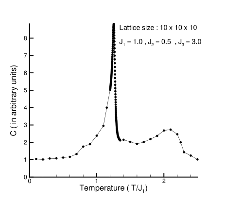
FIG. 1.: Temperature dependence of specific heat for $J_{1}=1.0$, $J_{2}=0.5$ and $J_{3}=3.0$. The points between $T=1.35$ and $T=1.2$ has been derived using multi-histogram method(see the text).

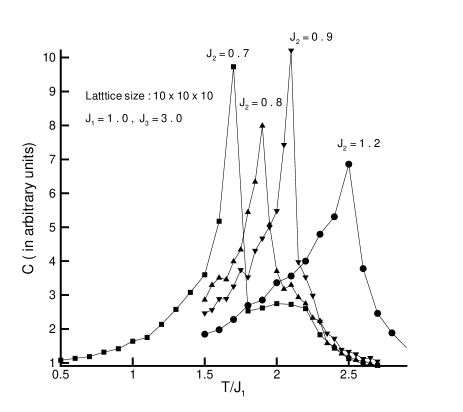
FIG. 2.: Temperature dependence of specific heat for $J_{1}=1.0$, $J_{3}=3.0$ and $J_{2}=0.7,0.8,0.9,1.2$

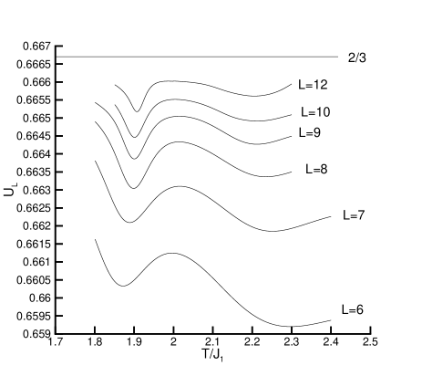
FIG. 3.: Binder’s fourth energy cumulant for $J_{1}=1.0$, $J_{2}=0.8$ and $J_{3}=3.0$. High temperature minima are near the transition from isotropic to hexatic while the low temperature minima indicate the transition from hexatic to hexatic+herringbone state.

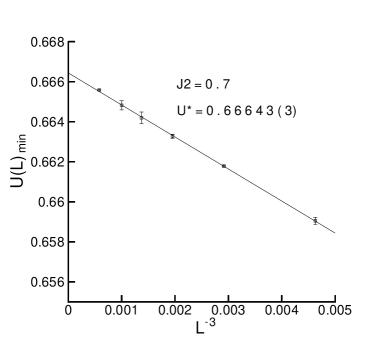
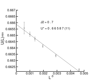
FIG. 4.: Size dependence of binder fourth energy cumulant minima, calculated by optimized re-weighting for $J_{1}=1.0$, $J_{2}=0.7$ and $J_{3}=3.0$.(a)Transition from isotropic to hexatic phase (second order),(b) transition from hexatic to hexatic+herringbone (first order). Solid lines represent fits to (17).

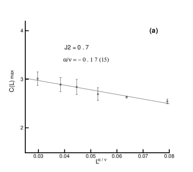
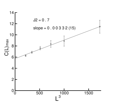
FIG. 5.: Size dependence of the specific heat maxima, $C_{max}$, calculated by optimized re-weighting for $J_{1}=1.0$, $J_{2}=0.7$ and $J_{3}=3.0$.(a)Transition from isotropic to hexatic phase,(b) transition from hexatic to hexatic+herringbone phases. Solid lines represent fits to (14) for (a) and (11) for (b) .

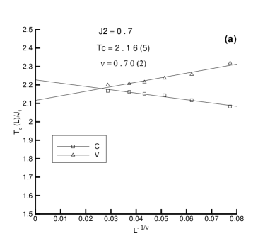
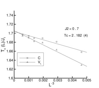
FIG. 6.: Scaling of the effective transition temperatures with lattice size. for $J_{1}=1.0$, $J_{2}=0.7$ and $J_{3}=3.0$. The $T_{c}$’s were obtained from the location of the maxima of specific heat and minima of Binder fourth energy cumulant. (a)Transition from isotropic to hexatic phase ,(b) transition from hexatic to hexatic+herringbone phases. The solid lines represent fits to (15) for (a) and (12) for (b).

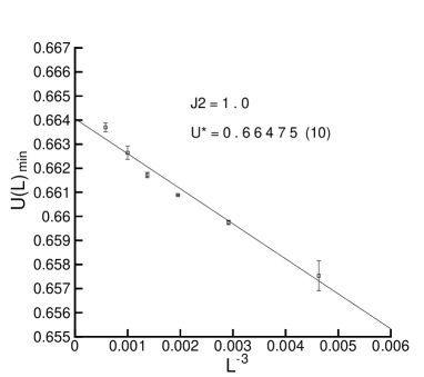
FIG. 7.: Size dependence of binder fourth energy cumulant minima, calculated by optimized re-weighting for $J_{1}=1.0$, $J_{2}=1.0$ and $J_{3}=3.0$ at the transition point from isotropic to hexatic+herringbone phases. Solid line represent fit to (17) the obtained value $U^{*}=0.66475(10)<2/3$ indicates a first order transition.

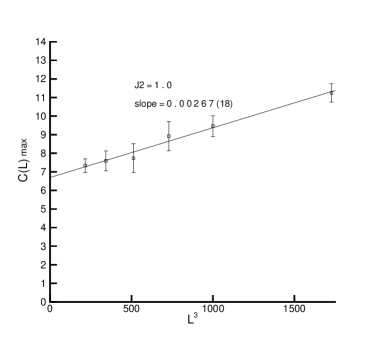
FIG. 8.: Size dependence of the specific heat maxima, $C_{max}$, calculated by optimized re-weighting for $J_{1}=1.0$, $J_{2}=1.0$ and $J_{3}=3.0$ at the transition point from isotropic to hexatic+herringbine phases. Solid line represents fit to (11).

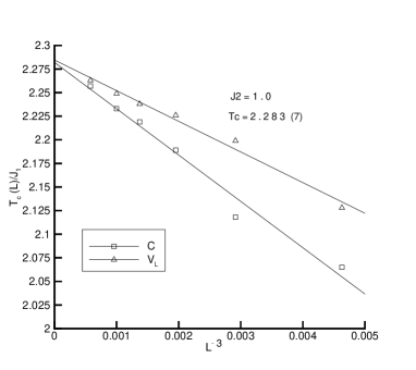
FIG. 9.: Scaling of the effective transition temperatures with lattice size, for $J_{1}=1.0$, $J_{2}=1.0$ and $J_{3}=3.0$. The $T_{c}$’s were obtained from the location of the maxima of specific heats and minima of Binder fourth energy cumulants. Solid lines represent fit (12).

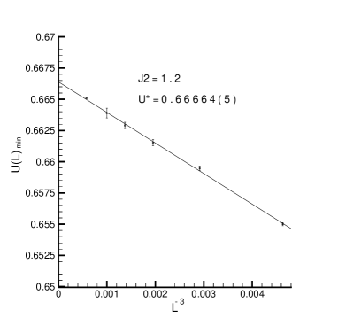
FIG. 10.: Size dependence of binder fourth energy cumulant minima, calculated by optimized reweighting for $J_{1}=1.0$, $J_{2}=1.2$ and $J_{3}=3.0$. Solid line represent fit to (17).

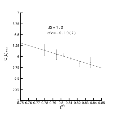
FIG. 11.: Size dependence of the specific heat maxima, $C_{max}$, calculated by optimized re-weighting for $J_{1}=1.0$, $J_{2}=1.2$ and $J_{3}=3.0$ at the transition point from isotropic to hexatic+herringbine phase. Solid line represents fit to (14), indicating a second order transition with negative value for specific heat anomaly exponent $\alpha$.

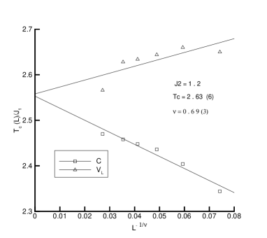
FIG. 12.: Scaling of the effective transition temperatures with lattice size. for $J_{1}=1.0$, $J_{2}=1.2$ and $J_{3}=3.0$. The $T_{c}$’s were obtained from the location of the maxima of specific heats and minima of Binder fourth energy cumulants. Solid lines represent fit (15) with value $0.69(3)$ for exponent $\nu$.

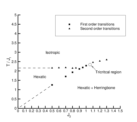
FIG. 13.: Schematic of the phase diagram obtained from simulation. Transition temperatures (in units of $J_{1})$ versus $J_{2}$. Three phases Isotropic, Hexatic and Hexatic+Herringbone has been shown and the dashed lines are just representing the separating of distinct phases. The region specified by circle is the tricritical region where order of the transition changes from being first order for $J_{2}=1.0$ to second order for $J_{2}=1.1$

REFERENCES

-
[1]
J. M. Kosterlitz and D. J. Thouless, J. Phys. C 6, 1181
(1973);
J. M. Kosterlitz, J. Phys. C 7, 1046 (1974) . -
[2]
B. I. Halperin and D. R. Nelson, Phys. Rev. Lett41, 121
(1978);
D.R. Nelson and B. I. Halperin, Phys. Rev. B 19, 2457(1979). - [3] A. P. Young, phys. Rev. B. 19, 1855 (1979).
- [4] K. J. Strandburg, Rev. Mod. Phys. 60, 161(1988)
- [5] R. J. Birgeneau and J. D. Lister, J. Phys. Paris. Lett 39, L339 (1978).
-
[6]
C. C. Huang and T. Stobe, Advances in Physics 42,343 (1993);
T. Stobe and C. C. Huang, Int. J. Mod. Phys B 9, 2285 1995. - [7] R. Pindak et al, Phys. Rev. Lett 46,1135 (1981).
- [8] C. C. Huang et al, Phys. Rev. lett 46,1289(1981).
- [9] T. Pitchford et al, Phys. rev. A 32,1938 (1985).
- [10] T. Stobe, C. C. Huang and J. W. Goodby, Phys. Rev. Lett. 68, 2944 (1992).
- [11] J. C. LeGuillou and J. Zinn Justin, J. Phys. Paris. Lett 46, L137 (1985) .
- [12] R. Bruinsma and G. Aeppli, Phys. Rev. Lett. 48, 1626 (1982).
-
[13]
M. J. P. Gingras, P. C. W. Holdworth and B. Bergersen, Europhys. Lett 9, 539 (1989);
ibid, Phys. Rev. A 41, 3377 (1990); ibid, Phys. Rev. A 41, 6786 (1990). - [14] M. J. P. Gingras, P. C. W. Holdworth and B. Bergersen, Mol. Cryst. Liq. Cryst. 204, 177(1991).
- [15] M. Kohandel, M. J. P. Gingras and J. P. Kemp, Phys. Rev. E. 68,41701(2003).
- [16] F. Shahbazi and M. J. P. Gingras, under preparation.
- [17] I. M. Jiang et al , Phys. rev. E 48, R3240 (1993).
- [18] I. M. Jiang, T. Stobe and C. C. Huang, Phys. Rev. Lett, 76,2910 (1996).
- [19] I. M. Jiang and C. C. Huang, Physica A, 221,104 (1995).
- [20] A. M. Ferrenberg and R. H. Swendsen, Phys. Rev. Lett, 63,1195 (1989).
- [21] D. P. Landau and K. Binder, A guide to monte carlo simulations in statistical physics, (Cambridge university press, 2000)
- [22] Murty. S. s. Challa and D. P. Landau, Phys. Rev. B, 34,1841 (1986).
- [23] J. Lee and J. M. Kosterlitz, Phys. Rev. B, 43,3265 (1991).