Emergence of hexatic and long-range herringbone order in two-dimensional smectic liquid crystals : A Monte Carlo study

Abstract

Using a high resolution Monte Carlo simulation technique based on multi-histogram method and cluster-algorithm, we have investigated critical properties of a coupled XY model, consists of a six-fold symmetric hexatic and a three-fold symmetric herringbone field, in two dimensions. The simulation results demonstrate a series of novel continues transitions, in which both long-range hexatic and herringbone orderings are established simultaneously. It is found that the specific-heat anomaly exponents for some regions in coupling constants space are in excellent agreement with the experimentally measured exponents extracted from heat-capacity data near the smecticA-hexaticB transition of two-layer free standing films.
PACS numbers: 61.30.-v, 64.70.Md

I Introduction

The mysterious critical properties of bulk and thin film liquid crystals at phase transition between smecteicA (SmA) phase with liquid like in-plane behaviour and HexaticB(HexB) phase with long-range bond orientational order but short range in-plane positional order, has been remained as a challenge for experimental and theoretical physicists after about 25 years.

The concept of hexatic phase was first introduced in two dimensional melting theory by Kosterlitz, Thouless, Halperin, Nelson and Young (KTHNY) [1],[2],[3]. According to this theory, two dimensional systems during melting transition from solid to isotropic liquid go through an intermediate phase called hexatic phase for systems that have six-fold(hexagonal) symmetry in their crystalline ground state. This hexatic phase displays short range positional order, but quasi long range bond-orientational order, which is different from the true long range bond-orientational and quasi long range positional order in 2D solid phases. It is known that for two dimensional systems, the transition from the isotropic liquid to hexatic phase could be either a KT transition or a first order transition [4].

The idea of hexatic phase was first applied to three dimensional systems by Birgeneau and Lister, who showed that some experimentally observed smectic liquid crystal phases ,consisting of stacked 2D layers, could be physical realization of 3D hexatics[5]. Assuming that the weak interaction between smectic layers could make the quasi long range order of two dimensional layers truly long ranged, they suggest that the 3D hexatic phases in highly anisotopic systems, possess short range positional and true long range bond-orientational order.

The first signs for the existence of the hexatic phase in three dimensional systems were observed in x-ray diffraction study of liquid crystal compound 65OBC(n-alkyl-4-m-alkoxybiphenyl-4-carboxylate,n=6,m=5)[6, 7], where a hexagonal pattern of diffuse spots was found in intensity of scattered x-rays. In addition to this hexagonal pattern, it was also found that some broader peaks were appeared in the diffracted intensity which indicate the onset of another ordering. These broad peaks are related to packing of molecules according to the herringbone structure perpendicular to the smectic layer stacking direction, although the range of herringbone ordering was not determined by a detailed investigation. The accompanying of the long range hexatic and herringbone orders make this phase a physically rich phase which simply is called Hexatic-B (HexB) phase. When temperature is decreased, the HexB phase transforms via a first order phase transition into the crystal-E (CryE) phase, which is a 3D plastic crystal exhibiting long range herringbone orientational ordering. Subsequently, it was found that other components in nmOBC homologous series (like 37OBC and 75OBC) and a number of binary mixtures of n-alkyl-4’-n-decycloxybiphenyl-4-carboxilate (n(10)OBC) with n ranging from 1 to 3 and also represent smA-HexB transition. In summary the most of $nm$OBC homologous series undergo the following bulk transition sequences Isotropic-SmA-HexB-CryE-CryK,where CryK is the rigid crystal structure, stable at room temperature.

The sixfold symmetry of hexatic phase suggests that bond-orientational order parameter to be defined by $\Psi_{6}=|\Psi_{6}|\exp(i6\psi_{6})$ describing the sixfold azimuthal modulation. The U(1) symmetry of the $\Psi_{6}$, implies that SmA-HexB transition be a member of XY universality class. However, heat capacity measurements on bulk samples of 65OBC [6, 8] and other calorimetric studies on many other components in the nmOBC homologous series [6, 9] have yielded very sharp specific heat anomalies near SmA-HexB transition with no detectable thermal hystersis and with very large value for the heat capacity critical exponent, $\alpha\approx 0.6$. These results indicate that this is a continues (second order) phase transition, but not belonging to The 3D XY universality class, for which the specific heat critical exponent is nearly zero ($\alpha\approx-0.007$[13]). On the other hand, the other static critical exponents determined from thermal conductivity ($\eta=-0.19$)and birefringence experiments ($\beta=0.19$) [6], all differ from the 3D XY values, indicating a novel phase transition with probably a new universality class.

These unusual behaviour also occurs in two dimensional liquid crystal compounds undergoing bulk hexatic transitions. The heat capacity measurement studies of (truly two-dimensional) two-layer free standing films of different nmOBC compound result a second order SmA-HexB transition, with a diverging specific-heat anomaly described by exponent $\alpha=0.31\pm 0.03$[6, 10]. This is obviously in contrast with the usual broad and nonsingular specific-heat hump of the KT transition far above $T_{c}$, predicted in two-dimensional melting theory. On the other hand, electron diffraction studies on $nm$OBC compound films revealed weak herringbone orders in hexatic phases, suggesting that SmA-HexB transition can not be described simply by a unique XY order parameter and the discrepancy between the experimental and two dimensional melting theory could be due to the presence of herringbone order in addition to bond-orientational order in such compounds.

In the light of these observations, Bruinsma and Aeppli[14] formulated a Ginzburg-Landau theory that included both hexatic and herringbone order. There are three inequivalent orientation for herringbone pattern on a triangular lattice, so the herringbone order parameter should be three-fold symmetric. Nevertheless, the broadness of x-ray diffracted peaks associated to herringbone order made Bruinsma and Aeppli to consider it short-ranged and associate an XY order parameter with two fold symmetry for herringbone ordering $(\Phi_{2}=|\Phi_{2}|\exp(i2\phi_{2}))$. Based on symmetry arguments, they also made a minimal coupling between the hexatic and herringbone order parameters as $V_{hex-her}=hRe(\Psi_{6}^{*}\Phi_{2}^{3})$. Microscopically, the origin of this coupling could be the anisotropy presented in liquid crystals molecular structures[15, 16].

In the mean field approach their results indicate that the SmA-HexB transition should be continuous. However one-loop renormalization calculations show that short range molecular herringbone correlations coupled to the hexatic ordering drive this transition first order, which becomes second order at a tricritical point[14]. Their result indicates the existence of two tricritical points, one for the transition between SmA phase ($\Psi=0,\Phi=0$) and the stacked hexatic phase ($\Psi\neq 0,\Phi=0$), and another for the transition between the SmA and the phase possessing both hexatic and herringbone order ($\Psi\neq 0,\Phi\neq 0$). Therefore, They concluded that the occurrence of phase transition near the tricritical points, with heat capacity exponent $\alpha=0.5$, would be a good explanation for large heat capacity exponents observed in the experiments. Recently, the RG calculation of BA model has been revised in [17] which resulted in finding another non-trivial fixed point missed in original work of Bruinsma and Aeppli. But it has been shown that this new fixed point is unstable in one loop level (order of $\epsilon$), which refuses this fixed point to represent a novel phase transition. Indeed, the limitations of RG methods which mostly rely on perturbation expansions, make them insufficient for accessing the strong coupling regimes where one expect that some kind of new treatment to appear. For this purpose, the numerical simulations would be useful.

The first numerical simulations for investigating the nature of the SmA-HexB transition in 2D systems have been done by Jiang et al who have used a model consists of a 2D lattice of coupled XY spins based on the BA Hamiltonian in strong coupling limit[19, 20]. Their simulation results suggest the existence of a new type phase transition in which two different orderings are simultaneously established through a continuous transition with heat capacity exponent $\alpha=0.36\pm 0.05$, in good agreement with experimental values. Recently, we have carried out a high-resolution Monte Carlo simulation, based on multi-histogram method, on BA model in three dimensions. Our results revealed the existence of a tricritical point on the transition line between SmA and hexatic+herringbone phases, but not any tricritical point on isotropic-Hexatic transition line[22].

However, While the occurrence of SmA-HexB in the vicinity of a tricritical point might be convincing reason for its observed large heat capacity exponents, some other questions remain unsolved. One question is that why seven different liquid crystal compounds nmOBC and five binary mixtures n(10)OBC, with very different SmA-HexB temperature ranges(which effect the coupling of two order types) yield approximately the same value $\alpha\approx 0.6$ and should all be in the immediate vicinity of a particular thermodynamic point. For example, the herringbone peaks observed in x-ray diffraction studies of 75OBC is weaker than those of 65OBC, hence if 65OBC is near a tricitical point then 75OBC should be further removed from this point. Yet the same specific-heat critical exponents has been obtained for these two compounds. The other problem concerns the mixture of 3(10)OBC (3-alkyl-4’-n-decycloxybiphenyl-4-carboxilate) and PHOAB (4-propionyl-4’-n-heptanoyloxyazo-benzene) compounds with PHOAB concentration between 30 and 70 percent, for which one expect very small herringbone fluctuations (because of large HexB temperature range) and therefore the SmA-HexB transition must be second order but a first order transition were found for these mixtures.

Therefore, this idea that the coupling of the hexatic order with short-ranged herringbone fluctuations is responsible for the unexpected critical behaviour of SmA-HexB transitions, has been faced with serious challenges by the above consideration. To best of our knowledge no detailed X-ray or electron diffraction studies have been done to determine the range of herringbone fluctuations, so it might not be truly short-ranged. On the other hand, the studies on thin-film heat-capacity data have suggested the probability of the existence of long-range herringbone order in a system with long-range bond orientational order and short-range transational order[6].

In views of the above remarks, we was motivated to investigate the critical properties of a coupled $XY$ model consisting of a hexatic order parameter with sixfold symmetry and a three-fold symmetric herringbone order. For this purpose we employed a high-resolution Monte Carlo technique to derive the critical temperatures and the critical exponents of this model over some ranges of coupling constants.

The rest of this paper is organized as follows. In section. II, we introduce model Hamiltonian and give a brief introduction to Wolf’s embedding method for reducing the critical slowing down and correlation between the measurements, the optimized Monte Carlo method based on multiple histograms and also Some methods for analyzing the Monte Carlo data to determine the order of transitions, critical temperatures and critical exponents. The simulation results and discussion is given in section III and conclusions will appear in section IV.

II Monte Carlo simulation

A Model

Recalling the six-fold symmetry of hexatic order and two-fold symmetry of the long range herringbone order, the Hamiltonian which describes both orderings ought to be invariant with respect to the transformation $\Phi\rightarrow\Phi+n(2\pi/3)$ and $\Psi\rightarrow\Psi+m(2\pi/6)$ where $n$ and $m$ are integers. Thus to lowest order in $\Psi$ and $\Phi$, one can write the following Hamiltonian for this model:

$$H= - J_{1}\sum_{<ij>}\cos(\Psi_{i}-\Psi_{j})-J_{2}\sum_{<ij>}\cos(\Phi_{i}-\Phi_{j})$$ (1)

$$- J_{3}\sum_{i}\cos(\Psi_{i}-2\Phi_{i}),$$ (2)

where the coefficients $J_{1}$ and $J_{2}$ are the nearest-neighbor coupling constants for the bond-orientational order $(\Psi)$ and herringbone order $(\Phi)$, respectively. The coefficient $J_{3}$ denotes the coupling strength between these two types of order at the same 3D lattice site. we are interested in situations in which $\Psi$ and $\Phi$ are coupled relatively strongly. Therefore for the beginning we fixed $J_{3}=2.0$,larger that both $J_{1}$ and $J_{2}$ for all the simulations. Assuming $J_{1}$ much larger than $J_{2}($ $J_{1}>>J_{2}$), for sufficiently high temperatures,(say $T>J_{3}$), the system is in completely disordered phase. For $T_{c1}<T<J_{3}$, the system remains disordered but the phases of the two order parameters become coupled through the herringbone-hexatic coupling term $J_{3}$. because of the XY symmetry of bond-orientational order ,for $T_{c2}<T<T_{c1}$ the hexatic order is first established through a KT transition and one would expect the ordered state to be correspondent to $\Psi_{i}\approx\Psi_{j}$ for all sites i and j, producing two degenerate minima for the free energy. So for these range of temperatures, the above Hamiltonian describes a system with the symmetry of the 2d-Ising model and then the transition between the pure hexatic ($\Psi\neq 0,\Phi=0$)and locked phase (hexatic plus long range herringbone ) ($\Psi\neq 0,\Phi\neq 0$) should be Ising-like at $T_{c2}$ with critical properties of 2d-Ising model. Thus for $J_{2}<<J_{1}<J_{3}$ the model exhibits an KT transition at $T_{c1}\sim{\pi J_{1}\over 2}$ and an Ising-like transition upon decreasing the temperature down to $T_{c2}\sim 2.7J_{2}$ ($k_{B}=1$). For $J_{2}\approx{\pi J_{1}\over 5.4}\approx 0.58J_{1}$, the two transition temperatures turn out to be equal and so a single transition occurs between disordered and locked phase in which two orderings would be established simultaneously.

For $0.58J_{1}<J_{2}<J_{3}$ the herringbone order would establish first and cause the correspondent field $\Phi$ to take nearly the same value for all sites. Because of this, the coupling term $J_{3}$ acts like a field on $\Psi$ and so the hexatic order parameter takes a nonzero value. So for this range of coupling constants the long range herringbone ordering will induce hexatic order at the same time.

To obtain a qualitative picture of transitions and also the approximate location of the critical points, we first set a low resolution simulations. The Simulations were carried out using standard Metropolis spin-flipping algorithm with lattice size $L=20\times 20$. During each simulation step, The angles $\Psi_{i}$ and $\Phi_{i}$ were treated as unconstrained, continuous variables. The random-angles rotations ($\Delta\Psi_{i}$ and $\Delta\Phi_{i}$) were adjusted in such a way that roughly $50\%$ of the attempted angle rotations were accepted. To ensure thermal equilibrium, 100 000 Monte Carlo steps (MCS) per spin were used for each temperature and 200 000 MCS were used for data collection. The basic thermodynamic quantities of interests are the specific heat $c=(\langle E^{2}\rangle-\langle E\rangle^{2})/(T^{2}L^{2})$, the herringbone order parameter $M=L^{-2}[(\sum_{i}\cos(\Phi_{i}))^{2}+(\sum_{i}\sin(\Phi_{i}))^{2}]$ and the susceptibility $\chi=(\langle M^{2}\rangle-\langle M\rangle^{2})/(TL^{2})$.

We have obtained the specific-heat,susceptibility and order parameter data as a function of temperature, shown in Fig. (1-3) for $J_{1}=1.0$ and $J_{2}=0.5,0.6,0.8,1.0$ and $J_{3}=2.0$. From the preceding discussion, it is clear that the small broad peaks near $T=1.1$ in figures (1) and (2) signal the XY transition due to the $J_{1}$ term, while the sharp peak located at $T\sim 0.9$ is expected to signal a transition into the state of 2d-Ising symmetry. For $J_{2}>0.6$, as already mentioned, only one sharp peak is observed in the specific-heat and susceptibility data which verifies our argument that for these values of $J_{2}$, the transition from disordered to long range herringbone ordered phase, simultaneously induces hexatic ordering.

B Wolff’s embedding trick

One important problem in Monte Carlo simulation, especially for large systems, is critical slowing down which is a major source of errors in measurements. To overcome the critical slowing down we used Wolff’s embedding technique[24]. This method is based on the cluster algorithm which originally proposed by Swendsen and wang for the potts model[23]. In Swendsen and Wang cluster algorithm a configuration of activated bonds is constructed from the spin configuration and after the clusters of spins are formed from configuration of bonds, the spin configuration is updated by assigning a randomly new spin value to each cluster and then the same value is given to all spins in the same cluster.

Wolff suggested a single-cluster algorithm in the way that only a single cluster grows from a randomly chosen site and then all the spins in the cluster are flipped. This single-cluster algorithm is very successful when applied to the Ising model[25].

Wolff further developed his technique For spin systems with continuous symmetry by introducing the Ising variable into $O(n)$ ferromagnetic models. Choosing a direction in the spin space at random each spin is projected onto that direction with two components, one perpendicular and the other either parallel or anti-parallel to the randomly chosen direction. An Ising model is then constructed by assigning $+1$ to to spins of parallel components and $-1$ to spins of anti-parallel components. The couplings between the nearest-neighbor Ising spins are determined by the products of these parallel and anti-parallel components and are therefore random in magnitude but are ferromagnetic. Such a random-bond Ising model can efficiently simulated with the single-cluster algorithm and the original $O(n)$ model can be correspondingly updated by changing the sign of parallel or anti-parallel components of spins in the same cluster[26, 31, 32].

For cluster updating of the coupled $XY$ model, we performed the following steps:

i)Choose a random oriented direction in 2-dimensional system with angle $\theta$ respect to $x$-axis and find the relative rotation of one of the two fields, i.e hexatic field ($\Psi$), respect to the randomly chosen direction ($\Psi^{\prime}_{i}=\Psi_{i}-\theta$);

ii)For each axis direction, generate independent random-bond Ising models for $\Psi$ variables by assigning $+1$ to each lattice point if $\cos(\Psi^{\prime}_{i})>0$ and $-1$ if $\cos(\Psi^{\prime}_{i})<0$ ;

iii) For each resultant random-bond Ising model correspondent to hexatic field, choose a lattice site randomly and build a single cluster with a bond-activating probability

$$P_{ij}=1-\exp(min(0,-2K_{1}\cos(\Psi^{\prime})_{i}\cos(\Psi^{\prime})_{j}),$$ (3)

where $K_{1}=J_{1}/T$ and the Boltzamann constant being 1;

iv) The spins in each cluster feel the effect of $\Phi$ fields through coupling term $J_{3}$. Once the $\Psi$ cluster is formed update the its configuration by flipping all correspondent embedded Ising variables in each cluster using Metropolis algorithm . For this purpose consider $\Delta E$ as energy difference of spin flipped and initial configurations for a given cluster in such a way that if $\Delta E<0$ all spins in the cluster will be flipped ($\Psi^{\prime}_{i}\rightarrow\pi-\Psi^{\prime}_{i}$) and if $\Delta E>0$ they will be flipped by probability $p=\exp(-K_{3}\Delta E$ in which $K_{3}=J_{3}/T$. Note that in this procedure all $\Phi$ variables remain unchanged.

v) Repeat (ii) to (iv) several times before going to next step;

vi)Now fix $\Psi$ variables and repeat steps (ii) to (v) for $\phi$ variables, Noting that in step (iii) $K_{1}$ should change to $K_{2}=J_{2}/T$.

vii) Turn to step (i) and choose a new random direction.

This multiple-updating scheme satisfies detailed balance and ergodicity and critical slowing down is reduced dramatically. To improve the quantity of data we combined the above algorithm with the single flip Metropolis method.

All simulations were carried out at five temperatures close to the effective transition points of the square lattices with linear sizes $L=20,24,28,32,36,40,50$ and $60$, by characterizing the corresponding peak position of the specific-heat and finite-lattice susceptibility. In each simulation $1\times 10^{5}$ cluster updating runs were carried out for equilibration. For data collection, $4\times 10^{5}$ measurements were made after enough single cluster-updating followed by single flip Metropolis runs are skipped (at least 10) to reduce the correlation between the measurements. Values of total energy and magnetization from each measurement were stored as a data list for histogram analysis.

C Histogram Method

To determine The location of the transition temperatures and other thermodynamic quantities such as specific heat near the transition points we need to use high resolution methods. For this purpose we used multiple-histogram reweighting method proposed by Ferrenberg and Swendsen [27], which makes it possible to obtain accurate data over the transition region from just a few Monte Carlo simulations. The central idea behind the histogram method is to build up information on the energy probability density function $P_{\beta}(E)$, where $\beta=1/T$ is inverse temperature (in units with $k_{B}=1$). A histogram $H_{\beta}(E)$ which is the number of spin configurations generated between $E$ and $E+\delta E$. $P_{\beta}(E)$ is defined as :

$$P_{\beta}(E_{i})=\frac{H_{\beta}(E_{i})}{Z_{\beta}},$$ (4)

where

$$Z_{\beta}=\sum_{i}H_{\beta}(E_{i}).$$ (5)

On the other hand we now that $P_{\beta}(E_{i})$ is proportional to the Boltzmann weight $\exp(-\beta E_{i})$ as:

$$P_{\beta}(E_{i})=\frac{g(E_{i})\exp(-\beta E_{i})}{Z_{\beta}},$$ (6)

in which $g(E_{i})$ is the density of states with energy $E_{i}$ and is independent of temperature. By knowing the probability distributions in a specific temperature, we can derive the density of states and find the probability distribution of energy at any temperature $\beta^{{}^{\prime}}$ as follows:

$$P_{\beta^{{}^{\prime}}}(E_{i})=\frac{P_{\beta}(E_{i})\exp[(\beta-\beta^{{}^{\prime}})E_{i}]}{\sum_{j}P_{\beta}(E_{j})\exp[(\beta-\beta^{{}^{\prime}})E_{j}]}.$$ (7)

In principle, $P_{\beta}(E)$ only provides information on the energy distribution of nearby temperatures. This is because the counting statistics in the wings of the distribution $H_{\beta}(E)$, far from the average energy at temperature $T$, will be poor.

To improve the estimation for density of states, one can take data at more than one temperature and combine the resultant histograms so as to take the advantages of the regions where each provide the best estimate for the density of states. This method has been studied by Ferrenberg and Swendsen who presented an efficient way for combining the histograms [27]. Their approach relies on first determining the characteristic relaxation time $\tau_{j}$ for the $j$th simulation and using this to produce a weighting factor $g_{j}=1+2\tau_{j}$. The overall probability distribution at coupling $K=\beta J$ obtained from $n$ independent simulation, each with $N_{j}$ configurations, is then given by :

$$P_{K}(E)=\frac{[\sum_{j=1}^{n}g_{j}^{-1}H_{j}(E)]e^{-KE}}{\sum_{j=1}^{n}N_{j}g_{j}^{-1}e^{-K_{j}E-f_{j}}},$$ (8)

where $H_{j}(E)$ is the histogram for the $j$th simulation and the factors $f_{j}$ are chosen self-consistently using Eq.(8) and

$$e^{f_{j}}=\sum_{E}P_{K_{j}}(E).$$ (9)

Thermodynamic properties are determined, as before, using this probability distribution, but now the results would be valid over a much wider range of temperatures than for any single histogram. In addition, this method gives an expression for the statistical error of $P_{K}(E)$ as:

$$\delta P_{K}(E)=[\sum_{j=1}^{n}g_{j}^{-1}H_{j}(E)]^{-1/2}P_{K}(E),$$ (10)

from which it is clear that the statistical error will be reduced when more MC simulations are added to the analysis.

To deal with thermodynamic quantities other than the energy, one can choose to to work with energy probability distribution and microcanonical averages of the quantities of interest. This leads to optimized use of computer memory. The microcanonical average of a given quantity $M$, which is a function of energy, can be calculated directly as :

$$M(E)=\frac{\sum_{t}M_{t}\delta_{E_{t},E}}{\sum_{t}\delta_{E_{t},E}},$$ (11)

from which the canonical average of $M$ can be obtained as a function of $T$:

$$\langle M\rangle=\frac{\sum_{E}M(E)P(E,T)}{\sum_{E}P(E,T)}.$$ (12)

The temperature dependence of thermodynamics quantities were determined by optimized multiple-histogram method. For all system sizes, histograms obtained from simulations overlap sufficiently on both sides of the critical point so that the statistical uncertainty in the wing of the histograms, near the critical point may be suppressed by using the optimized multiple-histogram method. Therefore the locations and magnitudes of the extrema of the thermodynamic quantities can be determined accurately to extract the critical temperature and static critical exponents from the finite-size scaling behaviour.

D Determination of $T_{c}$ and static critical exponents

In order to determinate the critical temperature in the infinite lattice sizes as well as the critical exponents, we use the finite-size scaling theory [33]. According to the finite-size scaling theory, the free energy density can be divided into a singular part $f_{s}$ and a background $f_{ns}$ which is non-singular as :

$$f(t,h;L)=f_{s}(t,h;L)+f_{ns}(t,L),$$ (13)

where $t=(T-T_{c})/T_{c}$ is the reduced temperature for a sufficiently large system at a temperature $T$ close enough to the infinite lattice critical point $T_{c}$ and $h$ is the external ordering field . Using the periodic boundary conditions makes The non-singular part size independent, leaving only the singular part of free energy for studying the critical properties of the system. The singular part is described phenomenologically by a universal scaling form

$$f(t,H;L)=L^{-d}Y(tL^{y_{t}},hL^{y_{h}})+\cdot\cdot\cdot,$$ (14)

where $d$ is the spatial dimension of the system and $y_{t}$ and $y_{h}$ are related to static critical exponents as $y_{t}=1/\nu$ and $y_{h}={\beta\delta\over\nu}$. Scaling form for various thermodynamic quantities can be obtained from proper derivations of the free energy density. Some of them such as magnetization density, susceptibility and specific heat in zero field are:

$$m \approx L^{\beta/\nu}{\mathcal{M}}(tL^{1/\nu})$$ (15)

$$\chi \approx L^{\gamma/\nu}{\mathcal{K}}(tL^{1/\nu})$$ (16)

$$c \approx c_{\infty}(t)+L^{\alpha/\nu}{\mathcal{C}}(tL^{1/\nu})$$ (17)

,

where $\alpha$ ,$\beta$,$\gamma$ and $\delta$ are static critical exponents. The Eqs(15-17) are used to estimate the critical exponents. But before dealing with the critical exponents we should first determine the critical temperature accurately.

The logarithmic derivatives are total magnetization ($mL^{d}$) are important thermodynamic quantities for studying critical phenomena and very useful to high accurate estimation of the critical temperature $T_{c}$ and the critical exponent $\nu$ [31]. For example defining the following quantities:

$$V_{1} \equiv 4[M^{3}]-3[M^{4}],$$ (18)

$$V_{2} \equiv 2[M^{2}]-[M^{4}],$$ (19)

$$V_{3} \equiv 3[M^{2}]-2[M^{3}],$$ (20)

$$V_{4} \equiv (4[M]-[M^{4}])/3,$$ (21)

$$V_{5} \equiv (3[M]-[M^{3}]/2,$$ (22)

$$V_{6} \equiv 2[M]-[M^{2}],$$ (23)

where $M=mL^{d}$ is the total magnetization of the system and

$$[M^{n}]\equiv\ln\frac{\partial\langle M^{n}\rangle}{\partial T}.$$ (24)

From Eq. (15) it is easy to show that

$$V_{j}\approx(1/\nu)\ln L+{\mathcal{V}}_{j}(tL^{1/\nu})$$ (25)

For $j=1,2,\cdot\cdot\cdot,6$. At the critical temperature ($t=0$) the ${\mathcal{V}}_{j}$ should be constants independent of the system size $L$. As we will see it gives us a very accurate tool to estimate both the critical temperature and correlation length exponent $\nu$ independently with high precision.

E Order of the transition

To determine the order of transitions, we used Binder’s forth energy cumulant defined as:

$$U_{L}=1-\frac{<E^{4}>}{3<E^{2}>}.$$ (26)

It has been shown that this quantity reaches a minimum at the effective transition temperature $T_{c}(L)$ whose size dependence is given by:

$$U_{min}(L)=U^{*}+BL^{-d}+O(L^{-2d}),$$ (27)

where

$$U^{*}=\frac{2}{3}-\left(e_{1}/e_{2}-e_{2}/e_{1}\right)^{2}/12.$$ (28)

The quantities $e_{1}$ and $e_{2}$ are the values of energy per site at the transition point a first order phase transition and $d$ is the spatial dimension of the system ($d=2$ in our simulation). Hence, for the continuous transitions for which there is no latent heat ($e_{1}=e_{2}$), in the limit of infinite system sizes, $U_{min}(L)$ tends to the value $U^{*}$ equal to $2/3$. For the first-order transitions, however $e_{1}\neq e_{2}$ and then $U^{*}$ reaches a value less than $2/3$ in the the limit $L\rightarrow\infty$. This method is actually a test for the Gaussian nature of the probability density function $P(E)$ at $T_{c}$. For a continuous transition, $P(E)$ is expected to be Gaussian at, as well as away from $T_{c}$. For a first-order transition, $P(E)$ will be double peaked in infinite lattice size limit, hence deviation from being Gaussian cause the minimum of $U_{L}$ tends $U^{*}$ to be less than $2/3$ as $L\rightarrow\infty$. This method is very sensitive, in a sense that small splitting in $P(E)$ for the infinite system that do not result in a double peak for small lattices can be detected.

III results and discossion

we are interested in investigating those region in coupling constants space for which the two kinds of ordernig establish together, so we limit ourselves to ${J_{2}\over J_{1}}>0.6$. Fixing $J3=1.0$ and $J_{3}=2.0$ we start to get data for $J_{2}=0.6,0.7,0.8,0.9,1.0$.

First of all we deal with the order of transitions. Employing the forth Binder energy cumulant method, discussed in previous section, we found that the order of transition for all values of $0.6\leq J_{2}\leq 1.0$ are second order in contrast to [18]. For example, we have plotted the size dependence of minimum values of $U_{L}$ ($U_{m}in(L)$ vs $L^{-2}$) for $J_{2}=0.6,0.8$ and $1.0$ in Fig.(4). As can be seen from this figure, the asymptotic values $U^{*}$ for all the $J_{2}$’s are equal to $2/3$ in the measurement errors, which indicate the continuous transition for these range of couplings.

After determining the order of transitions we proceed to estimate the critical temperatures and the critical exponents, using the finite-size scaling. The analysis discussed in section II.D provides a way to simultaneously determination of both $\nu$ and $T_{c}$. For this purpose, using Eq. (25) one can find the slope of quantities $V_{1}$ to $V_{6}$ (Eq. 18-23) versus $\ln(L)$ for the region near the critical point. Scanning over the critical region and looking for a quantity-independent slope gives us both the critical temperature $T_{c}$ and correlation length exponent $\nu$ with high precision. Figures (5) and (6) give the examples of such an effort for the set of the couplings ($J1=1.0,J2=0.8,J3=2.0$). From both figures we estimate that $\nu=0.837(5)$ and $T_{c}=1.157(1)$. The linear fits to the data in figure (5) has been obtained by the linear least square method. The similar procedure for couplings set ($J1=1.0,J2=1.0,J3=2.0$), shown in figures (7) gives $\nu=1.01(3)$ and $T_{c}=1.051(1)$.

Once $\nu$ and $T_{c}$ are determined accurately, we can extract other static critical exponents related to the order parameter ($\beta$) and susceptibility ($\gamma$). The ratio $\beta/\nu$ can be estimated by using the size dependence of the order parameter at the critical point given by Eq.(15). Figures (8) and (9) are log-log plots of the size dependence of the order parameter corresponding to field $\Phi$ for $J_{2}=0.6$ and $J_{2}=0.8$ respectively. From these figures the ratio $\beta/\nu$ can be estimated as the slope of the straight lines fitted to the data according to Eq.(15). We then have $\beta/\nu=.143(8)$ for $J_{2}=0.6$ and $\beta/\nu=.169(6)$ for $J_{2}=0.8$ and therefore $\beta=0.144(8)$ for $J2=0.6$ and $\beta=0.142(5)$ for $J_{2}=0.8$.

Accordingly, from Eq.(16) it is clear that the peak values of the finite-lattice susceptibility ($\chi=(\langle M^{2}\rangle-\langle M\rangle^{2})/(TL^{2})$) and the magnitude of the true susceptibility at $T_{c}$ (the same as $\chi$ with $\langle m\rangle=0$) are asymptotically proportional to $L^{\gamma/\nu}$ . So the slope of straight line fitted linearly to the log-log plot of these two quantities versus linear size of the lattices, can be calculated to estimate the ratio $\gamma/\nu$. Such plots have been depicted in Figures.(10) and (11) for $J2=0.6$ and $J2=0.8$, respectively. In Fig.(10), the slope of the bottom straight line (finite-lattice susceptibility) is $1.726(8)$ from the linear fit and the slope for the top one is $1.709(7)$, where the error includes the uncertainty in the slope resulting from uncertainty in our estimate for $T_{c}$. The ratio $\gamma/\nu$ obtained from the average of two slopes is $1.717$, therefore knowing the value of $\nu=1.01(3)$ one gets $\gamma=1.73(6)$ for $J2=0.6$ and $J3=2.0$. Similarly for $J_{2}=0.8$, depicted in Fig.(11), the slope of the bottom straight line (finite-lattice susceptibility) is $1.637(5)$ from the linear fit, while for the top one is $1.656(7)$, so he ratio $\gamma/\nu$ obtained from the average of the slopes is $1.656(9)$ which results in $\gamma=1.39(1)$ for $J2=0.8$ and $J3=2.0$.

Above procedure has been applied for other values of $J_{2}$ and the critical temperatures and critical exponents and for all values of herringbone couplings obtained in this work, have been listed in table.(1). In this table, the critical exponents $\alpha$, $\delta$ and $eta$ have been calculated using scaling laws:

$$\alpha = 2-d\nu$$ (29)

$$\gamma = \nu(2-\eta)=\beta(\delta-1)$$ (30)

on the other hand the Rushbrook scaling law ($\alpha+2\beta+\gamma=2$) is satisfied for all set of exponents in the computation errors.

In order to check the values of specific-heat anomaly exponents, we also estimated them independently, using size dependence of the specific-heat at measured critical temperatures according to Eq.(17). For this purpose we used least square method to find the best value of $\alpha/\nu$ to fit the heat capacity data at $T_{c}$. The plot of such efforts have been represented in figures () and () for $J_{2}=0.7$ and $J_{2}=0.8$ respectively, which resulted in $\alpha/\nu=45(2)$ for $J_{2}=0.7$ and $\alpha/\nu=0.39(1)$ for $J_{2}=0.8$. So knowing the obtained values of $\nu$, we find $\alpha=0.36(2)$ for $J_{2}=0.7$ and $\alpha=0.33(1)$ for $J_{2}=0.8$. This results are in very good agreement with the values obtained from Josefson scaling law.

One can see from table.(1) that the critical exponents for $J_{2}=0.6$ are close to two dimensional Ising model for which the exact exponents are $\alpha=0,\nu=1.0,\beta=0.125,\gamma=1.75,\delta=15$ and $\eta=0.25$. So $J_{2}=0.6$ is the onset of 2d-ising behaviour. By increasing the herringbone coupling constant, the thermal exponents $\alpha$ and $\nu$ differ dramatically from that of 2d-ising value. Heat capacity anomaly exponent $\alpha$ gets its maximum value ($\alpha=0.39$) for $J_{2}=0.7$ and then decreases to $0.22$ for $J_{2}=1.0$. The critical exponents for $J_{2}=0.9$ and $J_{2}=1.0$ are equal up to the simulation errors, hence these two belong to the same universality class.

The specific-heat exponent corresponding to $J_{2}=0.8$ ($\alpha=0.32(2)$) is the closest one to experimentally observed values ($\alpha=0.31\pm 0.03$). To investigate to sensibility of the critical exponents to hexatic-herringbone couplings we also measured the critical exponents for the coupling set $J_{1}=1.0,J_{2}=0.8$ and $J_{3}=1.0$. The static critical exponents obtained for this set of couplings are as $\alpha=0.31(3),\nu=0.845(15),\beta=0.13(2),\gamma=1.43(3),\delta=12.2(1.9)$ and $\eta=0.30(1)$. As we see again the heat capacity exponent is in excellent agreement with experimental value.

IV Conclusion

In summary, using the optimized Monte Carlo simulation based on multi-histogram and wolf’s embedding methods, we investigated the critical properties associated with a Hamiltonian containing two coupled XY order parameters (indicating a hexatic field with sixfold symmetry and a long-ranged herringbone field with twofold symmetry) in two dimensions. Unlike Bruinsma and Aeppli model, which possess the three state potts symmetry, the model proposed in this paper has 2d-Ising symmetry. However, static critical exponents derived by finite-size analysis for some range a coupling in coupling constants space, indicates clear deviations from two dimensional Ising behaviour in transition between isotropic to hexatic+herringbone phases. Our results show a non-universal characteristics along the transition line on which the two kinds of orderings would establish simultaneously. For the value of herringbone coupling ($J_{2}/J_{1}=0.6$), which is the onset of only one transition from disorder to locked phase, the critical behaviour is Ising-like, while by increasing the herringbone coupling the critical exponents begin to deviate from those of Ising values and finally reach to a new universality class correspond to $J_{2}/J_{1}=0.9$ and $J_{2}/J_{1}=1.0$ for which the exponents remain unchanged. Surprisingly for some values of herringbone couplings in between these to limit, i.e $J_{2}/J_{1}\sim 0.8$ and $J_{3}/J{1}=2.0,1/0$, the heat capacity exponents show very good agreement with experimentally observed values. Whether or not that these transitions are indicating a new universality or are just a crossover behaviour is an open problem and requires more theoretical investigations based on renormalization group theory.

Our results suggest that coupling of hexatic ordering to long-range herringbone packing but short-range translational ordering could give a plausible description for large specific-heat anomaly exponents of SmA-HexB transition in some liquid crystal compounds for which the herringbone ordering is accompany with the hexatic ordering. The confirmation of this idea requires the similar simulation in three dimensions and is the subject of our current research.

Experimentally, the accurate measurements of the range of herringbone ordering in HexB phase of $nm$OBC compounds in bulk and thin film samples and also measuring other static critical exponents rather than heat capacity exponent in thin film samples are also needed to check the validity of this model.

We finally hope that our work will motivate further theoretical, numerical and experimental investigations of this very interesting problem.

Acknowledgment We would like to thank prof. Hadi Akbarzadeh for letting us to use his computational facilities.

$J_{2}/J_{1}$	$T_{c}$	$\nu$	$\beta$	$\gamma$	$\alpha$	$\delta$	$\eta$
0.6	1.051(1)	1.01(3)	0.144(14)	1.73(6)	-0.02(6)	13.0(1.6)	0.282(8)
0.7	1.164(1)	0.806(9)	0.143(9)	1.31(3)	0.39(2)	10.1(9)	0.370(30)
0.8	1.257(1)	0.837(8)	0.142(5)	1.39(1)	0.32(2)	10.8(4)	0.344(9)
0.9	1.342(1)	0.886(3)	0.156(5)	1.46(1)	0.23(1)	10.3(4)	0.35(1)
1.0	1.423(1)	0.888(3)	0.150(4)	1.48(2)	0.22(2)	10.8(4)	0.33(1)

TABLE I.: The critical temperatures and static critical exponents for ${J_{2}\over J_{1}}=0.6,0.7,0.8,0.9,1.0$ and ${J_{3}\over J_{1}}=2.0$, derived from finite-size scaling.(see the text)

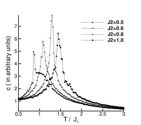
FIG. 1.: Temperature dependence of specific-heat for $J_{1}=1.0$, $J_{3}=2.0$ and $J_{2}=0.5,0.6,0.8,1.0$

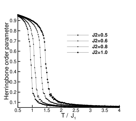
FIG. 2.: Temperature dependence of herringbobe order parameter for $J_{1}=1.0$, $J_{3}=2.0$ and $J_{2}=0.5,0.6,0.8,1.0$

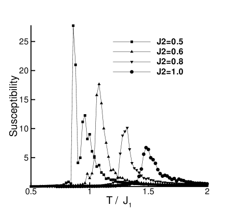
FIG. 3.: Temperature dependence of susceptibility for $J_{1}=1.0$, $J_{3}=2.0$ and $J_{2}=0.5,0.6,0.8,1.0$

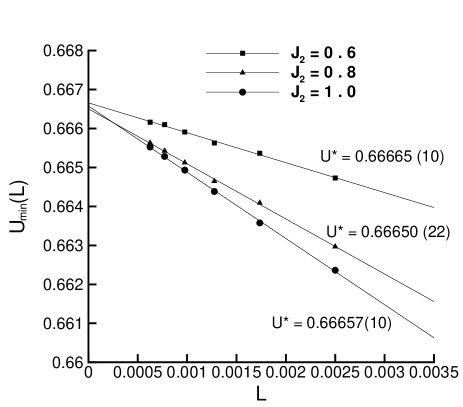
FIG. 4.: Size dependence of binder fourth energy cumulant minima, calculated by optimized re-weighting for $J_{1}=1.0$, $J_{3}=2.0$ and $J_{3}=0.6,0,8,1.0$ . Solid lines represent fits to (27). Error bars are less than the size of the points.

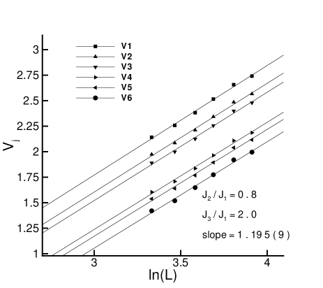
FIG. 5.: dependence of quantity $V_{j}$ (see the text) versus logarithm of $L$ for $J_{1}=1.0$, $J_{3}=2.0$ and $J_{2}=0.8$ at $T=1.258$. The solid lines represent linear fits to Eq.(25). All straight lines have the same slope $1.195$.

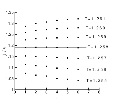
FIG. 6.: Scanning results for the dependence of quantity $V_{j}$ versus $j$ for $J_{1}=1.0$, $J_{3}=2.0$ and $J_{2}=0.8$. The horizontal line is drawn at $1/\nu=1.195$.

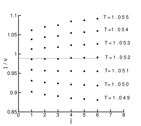
FIG. 7.: Scanning results of quantity $V_{j}$ for $J_{1}=1.0$, $J_{3}=2.0$ and $J_{2}=0.6$. The horizontal line is drawn at $1/\nu=0.99$.

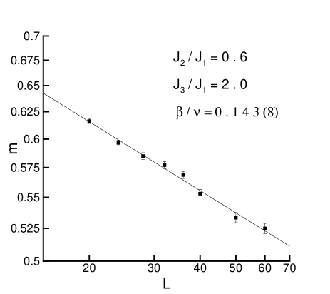
FIG. 8.: Log-log plot of order parameter versus the linear size of the lattice $L$ at $T_{c}=1.052$ for $J_{1}=1.0$, $J_{3}=2.0$ and $J_{2}=0.6$. The solid line is obtained by fitting the data to Eq(15).

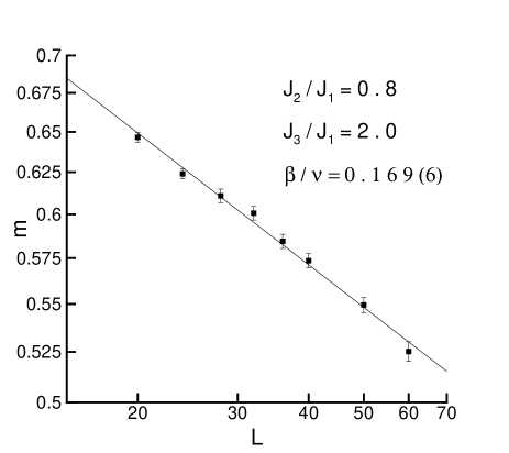
FIG. 9.: Log-log plot of order parameter versus the linear size of the lattice $L$ at $T_{c}=1.257$ for $J_{1}=1.0$, $J_{3}=2.0$ and $J_{2}=0.8$. The solid line is obtained by fitting the data to Eq(15).

FIG. 10.: Log-log plot of finite-lattice susceptibility and true susceptibility versus the linear size of the lattice $L$ at $T_{c}=1.052$ for $J_{1}=1.0$, $J_{3}=2.0$ and $J_{2}=0.6$. The solid line is obtained by fitting the data to Eq(16).

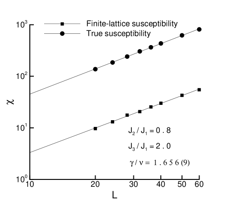
FIG. 11.: Log-log plot of finite-lattice susceptibility and true susceptibility versus the linear size of the lattice $L$ at $T_{c}=1.257$ for $J_{1}=1.0$, $J_{3}=2.0$ and $J_{2}=0.8$. The solid line is obtained by fitting the data to Eq(16).

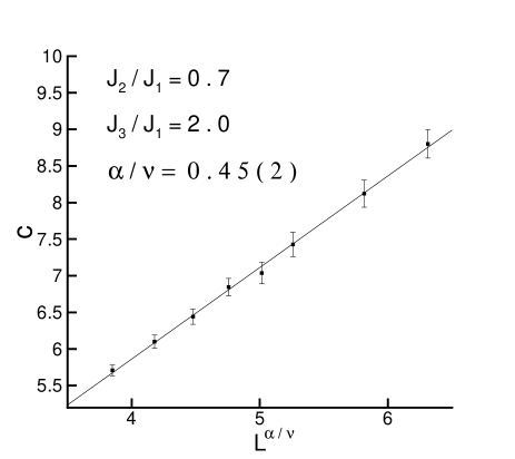
FIG. 12.: Size dependence of specific-heat at $T_{c}=1.164$ for $J_{1}=1.0$, $J_{3}=2.0$ and $J_{2}=0.7$. The solid line is obtained by fitting the data to Eq(17).

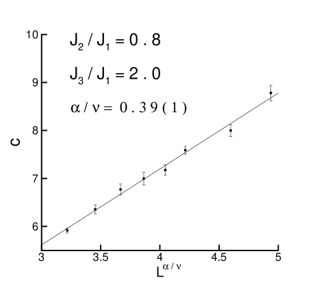
FIG. 13.: Size dependence of specific-heat at $T_{c}=1.257$ for $J_{1}=1.0$, $J_{3}=2.0$ and $J_{2}=0.8$. The solid line is obtained by fitting the data to Eq(17).

REFERENCES

-
[1]
J. M. Kosterlitz and D. J. Thouless, J. Phys. C 6, 1181
(1973);
J. M. Kosterlitz, J. Phys. C 7, 1046 (1974) . -
[2]
B. I. Halperin and D. R. Nelson, Phys. Rev. Lett41, 121
(1978);
D.R. Nelson and B. I. Halperin, Phys. Rev. B 19, 2457(1979). - [3] A. P. Young, phys. Rev. B. 19, 1855 (1979).
- [4] K. J. Strandburg, Rev. Mod. Phys. 60, 161(1988)
- [5] R. J. Birgeneau and J. D. Lister, J. Phys. Paris. Lett 39, L339 (1978).
-
[6]
C. C. Huang and T. Stobe, Advances in Physics 42,343 (1993);
T. Stobe and C. C. Huang, Int. J. Mod. Phys B 9, 2285 1995. - [7] R. Pindak et al, Phys. Rev. Lett 46,1135 (1981).
- [8] C. C. Huang et al, Phys. Rev. lett 46,1289(1981).
- [9] T. Pitchford et al, Phys. rev. A 32,1938 (1985).
- [10] T. Stobe, C. C. Huang and J. W. Goodby, Phys. Rev. Lett. 68, 2944 (1992).
- [11] A. J. Jin, M. Veum, T. Stobe, C. F. Chou, J. T. Ho, S. W. Hui, V. Surendranath and C. C. Huang, Phys. Rev. Lett. 74, 4863 (1995).
- [12] A. J. Jin, M. Veum, T. Stobe, C. F. Chou, J. T. Ho, S. W. Hui, V. Surendranath and C. C. Huang, Phys. Rev. E. 53, 3639 (1996).
- [13] J. C. LeGuillou and J. Zinn Justin, J. Phys. Paris. Lett 46, L137 (1985) .
- [14] R. Bruinsma and G. Aeppli, Phys. Rev. Lett. 48, 1626 (1982).
-
[15]
M. J. P. Gingras, P. C. W. Holdworth and B. Bergersen, Europhys. Lett 9, 539 (1989);
ibid, Phys. Rev. A 41, 3377 (1990); ibid, Phys. Rev. A 41, 6786 (1990). - [16] M. J. P. Gingras, P. C. W. Holdworth and B. Bergersen, Mol. Cryst. Liq. Cryst. 204, 177(1991).
- [17] M. Kohandel, M. J. P. Gingras and J. P. Kemp, Phys. Rev. E. 68,41701(2003).
- [18] E. Granato and J.M. Kosterlitz, Phys. Rev. B 33,4767 (1986).
- [19] I. M. Jiang et al , Phys. rev. E 48, R3240 (1993).
- [20] I. M. Jiang, T. Stobe and C. C. Huang, Phys. Rev. Lett, 76,2910 (1996).
- [21] I. M. Jiang and C. C. Huang, Physica A, 221,104 (1995).
- [22] R. Ghanbari and F. Shahbazi, Phys. Rev. E, 72, 021709 (2005).
- [23] R. H. Swendsen and J. S. Wang, Phys. Rev. Lett, 58, 86 (1987).
- [24] U. wolf, Phys. Rev. Lett, 62, 361 (1989);Nucl. Phys. B 322, 759 (1989).
- [25] P. Tamayo, R. C. Brower and w. Klein, J. Stat. Phys, 58, 1083 (1990).
- [26] D. Kandel and E. Domany, Phys. Rev. B, 43, 8539 (1991).
- [27] A. M. Ferrenberg and R. H. Swendsen, Phys. Rev. Lett, 63,1195 (1989).
- [28] D. P. Landau and K. Binder, A guide to monte carlo simulations in statistical physics, (Cambridge university press, 2000)
- [29] Murty. S. s. Challa and D. P. Landau, Phys. Rev. B, 34,1841 (1986).
- [30] J. Lee and J. M. Kosterlitz, Phys. Rev. B, 43,3265 (1991).
- [31] K. Chen, A.M. Ferrenberg and D. P. Landau, Phys. Rev. B, 48,3249 (1993).
- [32] P. Peczak, A.M. Ferrenberg and D. P. Landau, Phys. Rev. B, 43,6087 (1991).
- [33] M .N .Barber, Phase transitions and critical phenomena, edited by C. Domb and J. L. Lebowitz (Academic, New York, 1983), Vol. 8, p. 145.