Quantum instabilities in the system of identical bosons

Abstract

The quantum instability of the mean-field theory for identical bosons is shown to be described by an appropriate Bogoliubov transformation. A connection between the quantum and classical linear stability theories is indicated. It is argued that the instability rate in a system of identical bosons must be strongly affected by the nonlinear terms (interactions). In the case of the repulsive interactions or strong attractive interactions the instability rate is suppressed. On the other hand, a weak attraction significantly enhances the instability rate. The results can have applications in the field of Bose-Einstein condensates of dilute quantum gases.

Under some conditions, a quadratic Hamiltonian describing a system of identical bosons can be diagonalized by the Bogoliubov transformation BGLB . The physical sense of the diagonalization lies in a redefinition of the vacuum state and introduction of quasiparticles satisfying the boson commutation relations. The diagonalization is used, for instance, in description of the excitations in a Bose-Einstein condensate of dilute quantum gas BEC .

Diagonalization is not always possible which means that the quasiparticle excitations may give rise to an instability Anglin . Below it is shown that such instabilities are described by an appropriate Bogoliubov transformation which, however, is not related to the diagonalization procedure. Moreover, it is argued that even weak interactions (i.e. the higher-order terms) can cause a dramatic effect on the instability rate.

Driving a quantum many-body system through an instability region by changing the system parameters is an important tool in the quantum state engineering in BEC physics BEC , for instance, in the process of the atomic association ExpAtomAssoc1 ; ExpAtomAssoc2 ; TheorAtomAssoc1 and molecular dissociation in BEC QEffAtomMol ; QCurveCross2 . In a region of instability the mean-field theory breaks down TheorAtomAssoc1 ; QEffAtomMol ; QCorrMFT . The instability in system of identical bosons is also referred to as the curve crossing QCurveCross2 ; QCurveCross1 and is related to the Landau-Zener theory QCurveCross2 ; Anglin . In a condensate with the attractive interactions the quantum corrections are crucial for description of the dynamics when the mean field state is unstable BSB .

Let us first briefly recall the basics of the diagonalization procedure BGLB . Consider a Hamiltonian quadratic in the boson creation ($b_{j}^{\dagger}$) and annihilation ($b_{j}$) operators:

$$H=\sum_{k,l}A_{k,l}b^{\dagger}_{k}b_{l}+\frac{1}{2}\sum_{k,l}B_{k,l}b^{\dagger}_{k}b^{\dagger}_{l}+\frac{1}{2}\sum_{k,l}B^{*}_{k,l}b_{k}b_{l},$$ (1)

where $A^{\dagger}=A$ and $\tilde{B}=B$ (here $\dagger$, $\;{}_{\widetilde{}}\;$, and $*$ denote the Hermitian conjugation, the transposition, and the complex conjugation, respectively). The diagonalization of the Hamiltonian (1) introduces new boson operators, say $\xi^{\dagger}_{j}$ and $\xi_{k}$, such that the corresponding matrix $A$ becomes diagonal and $B$ vanishes.

The fact that the new operators satisfy the boson commutation relations together with the linearity and homogeneity of the transformation gives immediately the most general form of the Bogoliubov transformation:

$$\left(\begin{array}[]{c}\xi\\ \xi^{\dagger}\end{array}\right)=\left(\begin{array}[]{cc}U^{\dagger}&-V^{\dagger}\\ -\tilde{V}&\tilde{U}\end{array}\right)\left(\begin{array}[]{c}b\\ b^{\dagger}\end{array}\right),\quad U^{\dagger}U-V^{\dagger}V=I,\quad\tilde{U}V-\tilde{V}U=0.$$ (2)

Here, for simplicity, the index-free operators denote the whole column of such operators, e.g. $\xi\equiv(\xi_{1},\ldots,\xi_{n})$. Note that the conditions on matrices $U$ and $V$ in equation (2) also guarantee the existence of the inverse transformation

$$\left(\begin{array}[]{c}b\\ b^{\dagger}\end{array}\right)=\left(\begin{array}[]{cc}U&V^{*}\\ V&U^{*}\end{array}\right)\left(\begin{array}[]{c}\xi\\ \xi^{\dagger}\end{array}\right).$$ (3)

To diagonalize the Hamiltonian (1) the Bogoliubov transformation must be such that columns of the transformation in equation (3) are the eigenvectors of the following matrix eigenvalue problem

$$\left(\begin{array}[]{cc}I&0\\ 0&-I\end{array}\right)\left(\begin{array}[]{cc}A&B\\ B^{*}&A^{*}\end{array}\right)\left(\begin{array}[]{c}U_{\cdot,k}\\ V_{\cdot,k}\end{array}\right)=\lambda_{k}\left(\begin{array}[]{c}U_{\cdot,k}\\ V_{\cdot,k}\end{array}\right),$$ (4)

where $U_{\cdot,k}$ and $V_{\cdot,k}$ denote the $k$-th columns of the respective matrices. If the diagonalization is possible, the Hamiltonian (1) in the quasiparticle representation reads $H=\sum\lambda_{k}\xi^{\dagger}_{k}\xi_{k}-\sum\lambda_{k}\left(\sum_{l}|v_{l,k}|^{2}\right)$, where $v_{l,k}$ are the elements of the matrix $V$ BGLB . Note that the number of quasiparticles $N=\sum\xi^{\dagger}_{k}\xi_{k}$ is conserved.

The diagonalization procedure described above is closely related to the classical theory of stability of the stationary points of the Hamiltonian systems MacKay . Indeed, the second matrix on the l.h.s. of equation (4),

$$\mathcal{H}=\left(\begin{array}[]{cc}A&B\\ B^{*}&A^{*}\end{array}\right),$$ (5)

is the Hessian of the classical Hamiltonian system corresponding to the quantum Hamiltonian (1) when the boson operators $b$ and $b^{\dagger}$ are replaced by the $c$-numbers. Hence, the eigenvalues $\lambda_{k}$ of the eigenvalue problem (4) come in quartets $\{\lambda,\lambda^{*},-\lambda,-\lambda^{*}\}$. For the diagonalization to exist it is necessary that there are $n$ non-zero real eigenvalues and $n$ corresponding eigenvectors with the positive normalization, i.e. $U^{\dagger}U-V^{\dagger}V=I$.

The simplest sufficient condition for the diagonalization is the positivity of the corresponding Hessian. In the classical stability theory the quadratic form of the Hessian is the first non-zero term in the energy expansion, thus its positivity implies linear stability MacKay . The physical sense of the positivity of the Hessian is that the linearized system about the stationary solution is equivalent to a system of uncoupled oscillators (in the stationary case). In the quantum case the corresponding Hamiltonian, quadratic in boson operators, can be diagonalized. However, it is clear that the diagonalization is not always possible (for example, the Hamiltoian (6) below cannot be diagonalized when $|\delta|<\gamma$). In this case there no interpretation in terms of the uncoupled oscillators since the linearized system is hyperbolic.

A mean-field theory for bosons can be considered stable if the quasiparticle excitations remain bounded (for instance, when the Hessian is positive). There is a correspondence between the classical and quantum stability. Physically such a correspondence seems to be quite clear: due to the linearity of the Heisenberg evolution equations (for $b$ and $b^{\dagger}$) the stability in the classical sense implies that the diagonalization of the corresponding Hamiltonian, quadratic in boson operators, is possible. In the classical theory it is established that under a variation of the parameters the solution to a Hamiltonian system may become unstable due to collision of the imaginary eigenvalues with the energy of opposite signs (the opposite Krein signatures) or due to a collision of the eigenvalues at zero MacKay . Hence, the simplest quantum instability is due to a collision of two frequencies at a resonance.

The simplest example of the quantum instability (or non-diagonalizable boson Hamiltonian) has already appeared in the description of a boson system driven through a resonance QCurveCross1 ; QCurveCross2 ; Anglin . The corresponding Hamiltonian reads QCurveCross2 ; Anglin

$$H=[\omega+\delta(t)]a_{1}^{\dagger}a_{1}+[-\omega+\delta(t)]a_{2}^{\dagger}a_{2}+\gamma(a_{1}^{\dagger}a_{2}^{\dagger}+a_{1}a_{2}).$$ (6)

This Hamiltonian conserves the difference of the number of bosons: $[H,a_{1}^{\dagger}a_{1}-a_{2}^{\dagger}a_{2}]=0$. The total number of bosons is not conserved which is a reflection of the fact that the Hamiltonian (6) appears as a linearization of the full nonlinear Hamiltonian about the mean-field state or in the case of a macroscopically populated source of bosons. For instance, such a Hamiltonian appears in the description of the formation of atomic pairs by the dissociation of a molecular condensate QCurveCross1 ; QCurveCross2 . In the case of one highly populated molecular mode, while the atomic mode populations are not large, the model Hamiltonian is $H_{am}=[\omega+\delta(t)]\psi_{1}^{\dagger}\psi_{1}+[-\omega+\delta(t)]\psi_{2}^{\dagger}\psi_{2}+(g\Psi_{m}\psi_{1}^{\dagger}\psi^{\dagger}_{1}+g^{*}\Psi_{m}^{\dagger}\psi_{1}\psi_{2})$. If a macroscopic number of molecules does not change considerably, the annihilation operator for the molecular state can be approximated by an order parameter, $\Psi_{m}\to\langle\Psi_{m}\rangle$. Defining $\gamma=|g\langle\Psi_{m}\rangle|$ and $\psi_{j}=e^{i\chi}a_{j}$ with $\chi=\mathrm{arg}\{g\langle\Psi_{m}\rangle\}/2$ we obtain the Hamiltonian (6).

For the Hamiltonian (6) the corresponding Hessian reads

$$\mathcal{H}=\left(\begin{array}[]{cc}A&B\\ B^{*}&A^{*}\end{array}\right)=\left(\begin{array}[]{cc}\begin{array}[]{cc}\delta+\omega&0\\ 0&\delta-\omega\end{array}&\begin{array}[]{cc}\quad 0&\quad\gamma\\ \quad\gamma&\quad 0\end{array}\\ \begin{array}[]{cc}\quad 0&\quad\gamma\\ \quad\gamma&\quad 0\end{array}&\begin{array}[]{cc}\delta+\omega&0\\ 0&\delta-\omega\end{array}\end{array}\right).$$ (7)

The characteristic equation is bi-quadratic: $\lambda^{4}-2(\omega^{2}+\delta^{2}-\gamma^{2})\lambda^{2}+(\gamma^{2}-\delta^{2}+\omega^{2})^{2}=0$, it has the following four roots $\lambda=\pm(\omega\pm\sqrt{\delta^{2}-\gamma^{2}})$ (the two $\pm$ signs can be arbitrarily selected). Therefore the Hamiltonian (6) can be diagonalized for $|\delta|>\gamma$ by solving the eigenvalue problem (4). Setting $\sigma=\delta/\gamma$ one obtains the diagonalizing transformation

$$U=\left(\begin{array}[]{cc}u_{1}e^{i\theta_{1}}&0\\ 0&u_{1}e^{i\theta_{2}}\end{array}\right),\quad V=\left(\begin{array}[]{cc}0&u_{2}e^{i\theta_{2}}\\ u_{2}e^{i\theta_{1}}&0\end{array}\right),$$ (8)

with $\quad u_{1}=\left(1-[\sqrt{\sigma^{2}-1}-\sigma]^{2}\right)^{-1/2}$ and $u_{2}=[\sqrt{\sigma^{2}-1}-\sigma]u_{1}$ (without loss of generality, the arbitrary phases $\theta_{1,2}$ can be set to zero). In particular, the new boson operators read

$$\xi_{1}=e^{-i\theta_{1}}(u_{1}a_{1}-u_{2}a_{2}^{\dagger}),\quad\xi_{2}=e^{-i\theta_{2}}(u_{1}a_{2}-u_{2}a_{1}^{\dagger})$$ (9)

and the Hamiltonian reduces to

$$H=(\sqrt{\delta^{2}-\gamma^{2}}+\omega)\xi_{1}^{\dagger}\xi_{1}+(\sqrt{\delta^{2}-\gamma^{2}}-\omega)\xi_{2}^{\dagger}\xi_{2}+\sqrt{\delta^{2}-\gamma^{2}}-\delta.$$ (10)

When $\sigma=\delta/\gamma$ is time-independent the diagonalization decouples the Heisenberg evolution equations for the boson operators $\xi_{1}$ and $\xi_{2}$:

$$i\frac{\mathrm{d}\xi_{1}}{\mathrm{d}t}=(\sqrt{\delta^{2}-\gamma^{2}}+\omega)\xi_{1},\quad i\frac{\mathrm{d}\xi_{2}}{\mathrm{d}t}=(\sqrt{\delta^{2}-\gamma^{2}}-\omega)\xi_{2}.$$ (11)

Otherwise, there is no point in diagonalizing the Hamiltonian since the Bogoliubov transformation will be time-dependent and the evolution of the new boson operators $\xi_{1}$ and $\xi_{2}$ will be coupled (similar as the evolution equations for the original operators $a_{1}$ and $a_{2}$).

In the classical stability theory the Hessian (7) describes a collision of two eigenfrequencies at $|\delta|=\gamma$ ($\delta\to-\gamma$ from below or $\delta\to\gamma$ from above) with the appearance of complex eigenvalues (eigenfrequencies). This corresponds to the fact that the boson Hamiltonian (6) cannot be diagonalized for $|\delta|<\gamma$. The corresponding quantum instability can be thought as the exponential growth of the number of bosons, described by the boson operators $a_{1}$ and $a_{2}$, since the total number is not conserved.

Though the Hamiltonian cannot be diagonalized in the region of instability, the Bogoliubov transformation (2) plays an essential role in the solution of the Heisenberg evolution equations. This statement is valid for any quadratic Hamiltonian (1) and follows from the fact that the action of the corresponding time evolution operator on the boson creation and annihilation operators can be represented by an appropriate time-dependent Bogoliubov transformation (which is different from the diagonalizing transformation). The latter fact is just a consequence of the boson commutation relations for the creation and annihilation operators.

Let us consider the Hamiltonian (6) as an illustrative example. First one notes that $\omega$ can be eliminated by the unitary transformation with the generator $a_{1}^{\dagger}a_{1}-a_{2}^{\dagger}a_{2}$, which results in the substitution $a_{1}\to e^{i\omega t}a_{1}$ and $a_{2}\to e^{-i\omega t}a_{2}$ . Then, taking into account the symmetry of the transposition $a_{1}\leftrightarrow a_{2}$, the Bogoliubov transformation solving the Heisenberg evolution equations can be cast as

$$\left(\begin{array}[]{c}a\\ a^{\dagger}\end{array}\right)=\left(\begin{array}[]{cc}U^{\dagger}&-V^{\dagger}\\ -\tilde{V}&\tilde{U}\end{array}\right)\left(\begin{array}[]{c}a_{0}\\ a_{0}^{\dagger}\end{array}\right),\quad U=\left(\begin{array}[]{cc}{u}^{*}_{1}&0\\ 0&{u}^{*}_{1}\end{array}\right),\quad V=\left(\begin{array}[]{cc}0&-{u}^{*}_{2}\\ -{u}^{*}_{2}&0\end{array}\right).$$ (12)

The condition $U^{\dagger}U-V^{\dagger}V=I$ requires that $|u_{1}|^{2}-|u_{2}|^{2}=1$, while the second condition from equation (2) is satisfied identically. Differentiating equation (12) with respect to time and expressing the constant operators $a_{0}$ and $a_{0}^{\dagger}$ through the time-dependent operators $a$ and $a^{\dagger}$ by using the inverse Bogoliubov transformation one arrives at the following linear system for the parameters of the transformation

$$i\frac{\mathrm{d}}{\mathrm{d}t}\left(\begin{array}[]{c}u_{1}\\ {u}^{*}_{2}\end{array}\right)=\left(\begin{array}[]{cc}\delta(t)&\gamma\\ -\gamma&-\delta(t)\end{array}\right)\left(\begin{array}[]{c}u_{1}\\ {u}^{*}_{2}\end{array}\right).$$ (13)

A solution of system (13) determines the corresponding solution to the Heisenberg equations for the boson operators $a$ and $a^{\dagger}$. In fact, the latter equations can be obtained by the formal replacement: $u_{1}\to a_{1}$ and $u^{*}_{2}\to a^{\dagger}_{2}$. Note that the transformation defined by the solution of equation (13) has nothing to do with the diagonalization of the Hamiltonian.

System (13) formally coincides with the normalized classical system, which obtains from the Hamiltonian (6) by replacing the boson operators with $c$-numbers (equations (22) and (23) with $g=0$). The Hamiltonian (6) can also be cast as a linear combination of generators of the group $SU(1,1)$ (in our case: $\mathcal{K}_{0}=(a^{\dagger}_{1}a_{1}+a^{\dagger}_{2}a_{2}+1)/2$, $\mathcal{K}_{+}=a^{\dagger}_{1}a^{\dagger}_{2}$ and $\mathcal{K}_{-}=a_{1}a_{2}$ with $[\mathcal{K}_{0},\mathcal{K}_{\pm}]=\pm\mathcal{K}_{\pm}$ and $[\mathcal{K}_{+},\mathcal{K}_{-}]=-2\mathcal{K}_{0}$), thus the quantum instability case is formally similar to the problem of parametrically forced quantum oscillator BZP1 . However, the physics is quite different. For instance, in the quantum instability case there no adiabatic frequencies in the region of instability. The time-dependent Bogoliubov transformation was first used in the solution of the forced oscillator problem in Ref. BZP2 .

System (13) is equivalent to the approach of Refs. Anglin ; QCurveCross2 . Let us show, for instance, how the asymptotic formula of Ref. Anglin , relating the boson operators at $t\to\pm\infty$ in the case $\delta(t)=\varkappa^{2}t$, appears in our approach. The first order system (13) is equivalent to a second order equation (satisfied by both $u_{1}$ and $u_{2}$). Setting $t=z/\alpha$ with $\alpha^{2}=2i\varkappa^{2}$ we get the equation for the parabolic cylinder (Weber) functions: SpecFun

$$\frac{\mathrm{d}^{2}u_{k}(z/\alpha)}{\mathrm{d}z^{2}}+\left[-\frac{z^{2}}{4}+\nu+\frac{1}{2}\right]u_{k}(z/\alpha)=0$$ (14)

with $\nu=i\gamma^{2}/2\varkappa^{2}$. Using the simplified version of the integrating Bogoliubov transformation

$$\left(\begin{array}[]{c}a_{1}\\ a_{2}^{\dagger}\end{array}\right)=\left(\begin{array}[]{cc}u_{1}&u_{2}\\ {u}^{*}_{2}&{u}^{*}_{1}\end{array}\right)\left(\begin{array}[]{c}a_{10}\\ a_{20}^{\dagger}\end{array}\right),$$ (15)

the asymptotic conditions $u_{1}\to 1$ and $u_{2}\to 0$ as $ze^{-i\pi/4}\to-\infty$ complemented with the asymptotics of the first derivative derived from equation (13) and the standard asymptotic formulae for the parabolic cylinder functions one can arrive at the asymptotic formula of Ref. Anglin :

$$a_{k}(+\infty)=e^{\pi\gamma^{2}/2\varkappa^{2}}a_{k}(-\infty)+e^{i\eta}[e^{\pi\gamma^{2}/\varkappa^{2}}-1]^{1/2}a^{\dagger}_{k^{\prime}}(-\infty),$$

$$e^{i\eta}\equiv 2^{-i\gamma^{2}/2\varkappa^{2}}e^{-i\pi/4}\left[\frac{\Gamma(1-i\gamma^{2}/2\varkappa^{2})}{\Gamma(1+i\gamma^{2}/2\varkappa^{2})}\right]^{1/2},$$ (16)

with $k^{\prime}=2$ for $k=1$ and $k^{\prime}=1$ for $k=2$.

It is noted that formula (16) resembles the well-known Landau-Zener formula LZ (where the Weber functions also play the key role, see for instance Ref. LZ1 ). However, the quantum instability due to a collision of two eigenfrequencies is completely different from the Landau-Zener problem. This is manifested by our system (13). Indeed, system (13) resembles the Landau-Zener system but the evolution matrix on the r.h.s. of equation (13) is not Hermitian and the normalization condition for the “wave vector” $(u_{1},u_{2})$ is formulated in the Minkowsky space rather than in the Euclidian one. One consequence is that, as distinct from the Landau-Zener case, there is no equivalent of the adiabatic transition for slow time dependence of $\sigma=\delta/\gamma$, since the boson system passes through a region ($|\delta|<\gamma$) where the diagonalized Hamiltonian (10) is invalid. In other words, there is no adiabatic eigenfrequencies slowly depending on time in the region of $|\delta|<\gamma$, instead the system is hyperbolic with the solution given by a combination of the exponents $e^{\pm\sqrt{\gamma^{2}-\delta^{2}}t}$.

Therefore, the principal physical difference from the Landau-Zener problem lies in the fact that, due to the very instability that system (13) describes, the number of bosons grows in time and their interaction cannot be neglected at all times, in general. Let us consider what effect the interactions may have on the instability rate. Remembering that the Hamiltonian (6) appears as an approximation to the full nonlinear Hamiltonian (for instance, with the binary atomic collision term in the case of molecular dissociation) and eliminating the $\omega$ by $a_{1}\to a_{1}e^{i\omega t}$ and $a_{2}\to a_{2}e^{-i\omega t}$ one arrives at the simplest non-quadratic Hamiltonian describing the instability and interactions

$$H=\delta(t)(a_{1}^{\dagger}a_{1}+a_{2}^{\dagger}a_{2})+\gamma(a_{1}^{\dagger}a_{2}^{\dagger}+a_{1}a_{2})+g_{11}(a_{1}^{\dagger}a_{1})^{2}+g_{12}a_{1}^{\dagger}a_{1}a_{2}^{\dagger}a_{2}+g_{22}(a_{2}^{\dagger}a_{2})^{2}.$$ (17)

Below, for simplicity, we will set all the interaction coefficients equal, $g\equiv g_{11}=g_{12}=g_{22}$. The Heisenberg evolution equations written for the operators $\hat{a}_{1}=e^{-igKt}a_{1}$ and $\hat{a}_{2}^{\dagger}=e^{-igKt}a_{2}^{\dagger}$, with $K=a^{\dagger}_{1}a_{1}-a^{\dagger}_{2}a_{2}$, read

$$i\frac{\mathrm{d}}{\mathrm{d}t}\left(\begin{array}[]{c}\hat{a}_{1}\\ \hat{a}_{2}^{\dagger}\end{array}\right)=\left(\begin{array}[]{cc}\delta(t)+g+3g\hat{n}_{1}&\gamma\\ -\gamma&-\delta(t)-g-3g\hat{n}_{2}\end{array}\right)\left(\begin{array}[]{c}\hat{a}_{1}\\ \hat{a}_{2}^{\dagger}\end{array}\right),$$ (18)

where $\hat{n}_{1}=\hat{a}_{1}^{\dagger}\hat{a}_{1}$ and $\hat{n}_{2}=\hat{a}_{2}^{\dagger}\hat{a}_{2}$.

System (18) is equivalent to an infinite-dimensional linear system of equations arising in the Fock representation of the Schrödinger equation with the Hamiltonian (17). It turns out that a satisfactory numerical simulation of such a system requires a large number of the Fock modes to be used (about 10 000) due to the spreading of the excitations over a large number of the Fock amplitudes. This is in contrast to the linear case ($g=0$) when the corresponding infinite dimensional system in the Fock space is equivalent to the finite-dimensional system (13) for the parameters of the the Bogoliubov transformation.

Therefore, in the nonlinear case one has to rely on an approximate system. Our approximation is based on the replacement of the number operators $\hat{n}_{1}$ and $\hat{n}_{2}$ in equation (18) by their averages. Then the evolution of the boson operators $\hat{a}_{1}$ and $\hat{a}_{2}^{\dagger}$ must be given by an appropriate Bogoliubov transformation. The parameters of the corresponding Bogoliubov transformation satisfy the system

$$i\frac{\mathrm{d}}{\mathrm{d}t}\left(\begin{array}[]{c}\hat{u}_{1}\\ \hat{u}^{*}_{2}\end{array}\right)=\left(\begin{array}[]{cc}\delta(t)+g+3g\langle\hat{n}_{1}\rangle&\gamma\\ -\gamma&-\delta(t)-g-3g\langle\hat{n}_{2}\rangle\end{array}\right)\left(\begin{array}[]{c}\hat{u}_{1}\\ \hat{u}^{*}_{2}\end{array}\right).$$ (19)

Equation (15) (with all $a$ replaced by $\hat{a}$) provides the expression for the boson operators through their initial values. Using it one arrives at the following expressions for the averages:

$$\langle\hat{n}_{1}\rangle=|\hat{u}_{1}|^{2}\langle\hat{n}_{10}\rangle+|\hat{u}_{2}|^{2}(\langle\hat{n}_{20}\rangle+1),\quad\langle\hat{n}_{2}\rangle=|\hat{u}_{1}|^{2}\langle\hat{n}_{20}\rangle+|\hat{u}_{2}|^{2}(\langle\hat{n}_{10}\rangle+1)$$ (20)

under the assumption that there is no initial pairing of the bosons: $\langle\hat{a}_{10}\hat{a}_{20}\rangle=0$. Using the normalization condition $|\hat{u}_{1}|^{2}-|\hat{u}_{2}|^{2}=1$ and making the phase transformation $\hat{u}_{1}=e^{3ig(\langle\hat{n}_{20}\rangle+1/2)t}u_{1}^{\prime}$ and $\hat{u}_{2}=e^{3ig(\langle\hat{n}_{20}\rangle+1/2)t}u_{2}^{\prime}$ we arrive at the nonlinear system

$$i\frac{\mathrm{d}}{\mathrm{d}t}\left(\begin{array}[]{c}u^{\prime}_{1}\\ {u^{\prime}}^{*}_{2}\end{array}\right)=\left(\begin{array}[]{cc}\delta(t)+g/2+3g(N_{0}+1)|u^{\prime}_{1}|^{2}&\gamma\\ -\gamma&-\delta(t)-g/2-3g(N_{0}+1)|u^{\prime}_{2}|^{2}\end{array}\right)\left(\begin{array}[]{c}u^{\prime}_{1}\\ {u^{\prime}}^{*}_{2}\end{array}\right),$$ (21)

where $N_{0}=\langle\hat{n}_{10}\rangle+\langle\hat{n}_{20}\rangle$.

At this point it is interesting to compare the approximate system (21) with the classical system resulting from the Hamiltonian (17) when the boson operators are replaced by the $c$-numbers:

$$H_{\mathrm{cl}}=\delta(t)[C^{*}_{1}C_{1}+C^{*}_{2}C_{2}]+\gamma[C^{*}_{1}C^{*}_{2}+C_{1}C_{2}]+g[(C^{*}_{1})^{2}C_{1}^{2}+C^{*}_{1}C_{1}C^{*}_{2}C_{2}+(C^{*}_{2})^{2}C_{2}^{2}].$$ (22)

The corresponding classical system reads

$$i\frac{\mathrm{d}}{\mathrm{d}t}\left(\begin{array}[]{c}C^{\prime}_{1}\\ {C^{\prime}}^{*}_{2}\end{array}\right)=\left(\begin{array}[]{cc}\delta(t)+3gK_{0}|C^{\prime}_{1}|^{2}&\gamma\\ -\gamma&-\delta(t)-3gK_{0}|C^{\prime}_{2}|^{2}\end{array}\right)\left(\begin{array}[]{c}C^{\prime}_{1}\\ {C^{\prime}}^{*}_{2}\end{array}\right),$$ (23)

where $C_{1}=e^{igK_{0}t}\sqrt{K_{0}}C_{1}^{\prime}$, ${C}^{*}_{2}=e^{igK_{0}t}\sqrt{K_{0}}{C^{\prime}}^{*}_{2}$, with $K_{0}=|C_{1}|^{2}-|C_{2}|^{2}$ being an integral of motion. Here $|C_{1}^{\prime}|^{2}-|C_{2}^{\prime}|^{2}=1$.

Systems (23) and (21) are similar. One difference between them lies in the definition of the nonlinearity coefficient. In the classical system it is proportional to the integral of motion, while in system (21) the nonlinearity coefficient is determined by the initial average of the total number of the bosons. (Note that for $K_{0}=0$ the correspondence between systems (23) and (21) cannot be established.) Another difference between the two systems lies in the physical sense of the variables. In the classical system $C^{\prime}_{k}$ are the (normalized) amplitudes of the perturbation about the mean-filed state, while in the case of system (21) $u_{k}$ are parameters of the Bogoliubov transformation which describes the evolution of the boson operators.

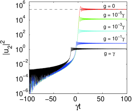
Figure 1: Numerical solution of the reduced system (21) in the case of repulsive interactions between the bosons. Here $\varkappa=0.5\gamma$. The dashed line is the asymptotic value of $\langle\hat{n}_{1}\rangle=|u_{2}|^{2}$ for $g=0$, according to formula (16).

Consider now the effect of nonlinearity on the quantum instability. Let us assume that the system is driven through the instability linearly, $\delta=\varkappa^{2}t$. Consider, for example, evolution of the system which was initially in the vacuum state (i.e. $N_{0}=\langle\hat{n}_{10}\rangle+\langle\hat{n}_{20}\rangle=0$) and far from resonance: $-t_{0}\gg\gamma/\varkappa^{2}$.

We are interested in the average values of the number operators, which, according to formula (20), in the case of $N_{0}=0$ read $\langle\hat{n}_{1}\rangle=\langle\hat{n}_{2}\rangle=|u_{2}|^{2}$.

We have found that in the case of the repulsive interactions between the bosons, $g>0$, the instability rate is significantly reduced and the asymptotic averages are lower by orders of magnitude, see fig 1. Note that even a weak repulsion has a dramatic effect on the resulting asymptotic number of the bosons.

In the case of the attractive interactions, $g<0$, the effect of a weak attraction consists in enhancing the production of the bosons, as seen from fig. 2. On the other hand, a strong attractive interaction decreases the instability rate.

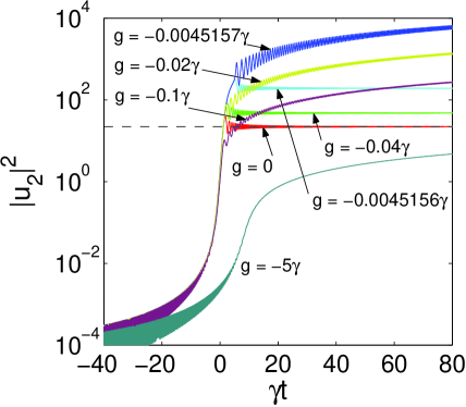
Figure 2: Numerical solution of the reduced system (21) in the case of attractive interactions between the bosons. Here $\varkappa=\gamma$. The dashed line is the corresponding asymptotic result for $g=0$. We have used $t_{0}=-100$.

In conclusion, it is shown that the quantum instability of the mean-field theory for identical bosons can be described by an appropriate Bogoliubov transformation. The relation to the instability in the corresponding classical system is established. We argue that a quantum instability in a system of identical bosons is strongly affected by the interactions. In the case of repulsion or strong attraction between the bosons the instability rate is suppressed. On the other hand, a weak attraction significantly enhances the instability rate. These results can have applications in the field of Bose-Einstein condensates of quantum gases.

References

- (1) N.N. Bogoliubov and N.N. Bogoliubov, Jr., Introduction to Quantum Statistical Mechanics, World Scientific Pub Co., 1982.
- (2) L. Pitaevskii and S. Stringari, Bose-Einstein Condensation, Clarendon Press, Oxford, 2003.
- (3) J.R. Anglin, Phys. Rev. A 67 (2003) 051601(R).
- (4) R. Wynar, R.S. Freeland, D.J. Han, C. Ryu, and D.J. Heinzen, Science 287 (2000) 1016.
- (5) J. Herbig, T. Kraemer, M. Mark, T. Weber, C. Chin, H.-C. N Agerl, and R. Grimm, Science 301 (2003) 1510.
- (6) M. Kostrun, M. Mackie, R. Côté, and J. Javanainen, Phys. Rev. A 62 (2000) 063616.
- (7) J.R. Anglin and A. Vardi, Phys. Rev. A 64 (2001) 013605.
- (8) A. Vardi, V.A. Yurovsky, and J.R. Anglin, Phys. Rev. A 64 (2001) 063611.
- (9) M.A. Kayali and N.A. Sinitsyn, Phys. Rev. A 67 (2003) 045603.
- (10) V.A. Yurovsky, A. Ben-Reuven, and P.S. Julienne, Phys. Rev. A 65 (2002) 043607.
- (11) G.P. Berman, A. Smerzi, and A.R. Bishop, Phys. Rev. Lett. 88 (2002) 120402.
- (12) R.S. MacKay, Stability of equilibria of Hamiltonian systems, in Nonlinear Phenomena and Chaos, ed. S. Sarkar, Hilger, Bristol, 1986, p. 254.
- (13) A.M. Perelomov and V.S. Popov, Sov. Phys. JETP 56 (1969) 1375; ibid 57 (1969) 1684; Teoret. Mat. Fiz. 3 (1969) 360.
- (14) A.I. Baz, Ya.B. Zeldovich and A.M. Perelomov, Scattering, Reactions and Decays in the Nonrelativistic Quantum Mechanics, Moscow, Nauka, 1971.
- (15) M. Abramowitz and I.A. Stegun, Handbook of Mathematical Functions, Dover, New York, 1964.
- (16) L.D. Landau, Phys. Z. Sowjetunion 2 (1932) 46; C. Zener, Proc. R. Soc. London A 137 (1932) 696.
- (17) N.V. Vitanov and B.M. Garraway, Phys. Rev. A 53 (1996) 4288.