Persistent currents in two dimensions:
New regimes induced by the interplay between electronic correlations and disorder

Abstract

Using the persistent current $I$ induced by an Aharonov-Bohm flux in square lattices with random potentials, we study the interplay between electronic correlations and disorder upon the ground state (GS) of a few polarized electrons (spinless fermions) with Coulomb repulsion. ${\bf K}$ being the total momentum, we show that $I\propto{\bf K}$ in the continuum limit. We use this relation to distinguish between the continuum regimes, where the lattice GS behaves as in the continuum limit and $I$ is independent of the interaction strength $U$ when ${\bf K}$ is conserved, and the lattice regimes where $I$ decays as $U$ increases. Changing the disorder strength $W$ and $U$, we obtain many regimes which we study using the map of local currents carried by three spinless fermions. The decays of $I$ characterizing three different lattice regimes are described by large $U$ perturbative expansions. In one of them, $I$ forms a stripe of current flowing along the axis of the diamagnetic Wigner molecule induced by large electronic correlations. This stripe of current persists in the continuum limit. The quantum melting of the diamagnetic molecule gives rise to an intermediate “supersolid” regime where a paramagnetic correlated pair co-exists with a third particle, before the total melting. The concepts of stripe and of supersolid which we use to describe certain regimes exhibited by three spinless fermions are reminiscent of the observations and conjectures done in other fields at the thermodynamic limit (stripe for high-Tc cuprates, supersolid for Helium quantum solids).

1 Introduction

1.1 Motivations

Let us first give some reasons which have motivated this study of a few polarized electrons (spinless fermions) and of their persistent current in two dimensional disordered lattice models. In the last decade, the conductance of two dimensional electron gases (2DEGs) have been measured abrahams at low temperatures as a function of their densities. Using 2DEGs created in Ga-As heterostructures or Si-MOSFETs at densities smaller than those used for studying the weak-localization corrections to the Drude-Boltzmann conductance, a “two dimensional metal-insulator transition” has been observed. When the temperature increases, the conductance does not change at a certain critical density, while it increases at smaller densities and decreases at larger densities. The increase corresponds to the insulating phase and the decay to the metallic phase. In Ga-As heterostructures or Si-MOSFETs, there is a more or less important disorder due to charged impurities and rough interfaces. In presence of disorder, a 2DEG can be insulating for two reasons: either because it forms a Fermi glass with Anderson localization at high densities or because it forms a pinned Wigner crystal at low densities. Since this transition is observed at low densities, it was suggested yoon that the low density insulator would be a pinned Wigner crystal, which would give an unexpected metal when it melts above the critical density. While a 2d insulator is expected, the observation of a 2d metal remains unexplained. If one goes simmons from the Fermi glass towards the pinned Wigner crystal via a 2d metal as the density decreases, the existence of a new metallic phase between two insulating phases of different nature becomes unavoidable. And indeed, exact numerical studies of small disordered clusters have shown bwp1 ; bwp2 ; avishai ; sp the trace of an intermediate regime consistent with this hypothesis.

Subsequent numerical studies of similar systems have shown ksp ; np that an intermediate regime persists without disorder. The possibility of having some hybrid phase made of a quantum solid co-existing with delocalized defects, was suggested in refs. ksp ; np , in analogy with the “supersolid” proposed long ago by Andreev and Lifshitz for quantum Helium solids in three dimensions andreev-lifshitz ; DKL . Using a similar analogy with Helium physics, but assuming macroscopic inhomogeneities of the carrier density due to an inhomogeneous substrate potential, a qualitative explanation of the dependence of the resistance as a function of a parallel magnetic field and of the temperature has been discussed in Ref. spivak1 .

For a simple 2DEG without a random substrate, to understand how the ground state (GS) changes when one varies the carrier density remains a challenge despite a few decades of efforts. The simplest model for a 2DEG is a continuum Hamiltonian $H_{c}$ having three parts: one body kinetic terms, a two body Coulomb repulsion and a one body potential describing the effect of the positive ions. The last potential is necessary to have a stable system of electrons because of Coulomb repulsions. However, if one takes periodic boundary conditions (BCs) and a uniform jellium for the positive ions, the corresponding potential becomes a constant term. The scale of the one body quantum effects is given by the Bohr radius $a_{B}=\hbar^{2}/me^{2}$, $e$ and $m$ being the electronic charge and mass. The strength of the Coulomb repulsion depends on the radius $a$ of a circle which encloses on the average one electron. Measuring the energies in rydbergs ($1Ry=me^{4}/2\hbar^{2}$) and the lengths in units of $a$, the continuum 2DEG Hamiltonian for $N$ electrons reads

$$H_{c}=-\frac{1}{r_{s}^{2}}\sum_{i=1}^{N}\nabla_{i}^{2}+\frac{2}{r_{s}}\sum_{1\leq i<j\leq N}\frac{1}{|{\bf r}_{i}-{\bf r}_{j}|}+const,$$ (1)

which only depends on a single scaling ratio

$$r_{s}=\frac{a}{a_{B}}$$ (2)

when $N\rightarrow\infty$. We neglect the spin degrees of freedom, considering fully polarized electrons (spinless fermions). Even in this simpler case, the interplay between Coulomb repulsion and the kinetic energy is a complicated issue. When many electrons are inside the quantum volume $a_{B}^{2}$, $r_{s}$ is small and the 2DEG is a Fermi liquid, with a Fermi energy much larger than the Coulomb energy. When $r_{s}$ is large, the volume per electron $a^{2}$ is large compared to $a_{B}^{2}$, and one has an electron solid (Wigner crystal) with weak quantum effects. Between those two limits, the nature of the ground state remains unclear.

From Quantum Monte Carlo studies, it is generally believed that there is a single first order liquid-solid transition. However this result is not free of certain assumptions, because of the well known “sign problem” of the Monte Carlo methods applied to fermions. One reason to question the existence of a single transition comes from general considerations about Landau theory of phase transitions and estimates of interface energies. According to Ref. spivak2 , a single first order transition is ruled out because a macroscopic phase separation between a liquid and a solid is unstable. A way to fix the sign problem of the Monte Carlo approaches consists in imposing the GS nodal structure. Using a fixed node approach, two nodal structures (a Slater determinant of plane waves for the liquid, of localized orbitals for the solid) have been compared ceperley , giving $r_{s}^{W}\approx 37$ for the critical density at which the transition occurs between the two assumed nodal structures. However, one cannot exclude the existence of better nodal structures giving lower GS energies when $r_{s}$ is neither small nor large. And indeed, a third nodal structure has been recently studied fw ; f in a fixed node Monte Carlo approach, using Bloch waves in a variational attractive potential located at the sites of the Wigner lattice instead of free plane waves. This third nodal structure gives a lower GS energy for $30<r_{s}<80$ and $N\rightarrow\infty$, supporting the existence of a new hybrid liquid-solid phase. Since one does not know the nodal structures, the Monte Carlo methods make problem, and exact numerical studies of small systems remain useful, despite the presence of large finite size effects. They could provide a better understanding of the low energy physics of a 2DEG, suggesting better trial wave functions for fixed node Monte Carlo methods. Or they could be the starting point of a finite size scaling theory bwp3 for the interacting 2DEG. This is the road which we have explored in a series of works bwp1 ; bwp2 ; sp ; ksp ; np ; mp ; fnp and which we continue here.

To do an exact study, we take $N$ electrons on a $L\times L$ lattice for having an Hilbert space of finite size. If $N$ and $L$ are small enough, the GS can be obtained by Lanczos algorithm. Beside the finite size effects due to the finite value of $N$, one has the lattice effects due to the finite value of $L$. If the lattice effects are irrelevant, the lattice GS behaves as the continuum GS. Notably, the parameter $r_{s}$ remains a scaling parameter. If the lattice effects are relevant, $r_{s}$ becomes meaningless, the scaling behavior of the continuum limit ceases to exist for giving rise to a new lattice physics. In the absence of disorder, the lattice effects were studied fnp as a function of the strength $U$ of the Coulomb repulsion. The strength $U^{*}$ above which the lattice GS and the continuum GS become different was given. The previous studies of a few particle systems ksp ; np ; fnp give the following picture: If one increases $U$ for a sufficiently small number $N$, the Fermi system disappears above $U^{F}$ to become a Wigner solid above $U^{W}$, through an intermediate regime for $U^{F}<U<U^{W}$ which could be the microscopic trace of an “electron supersolid”, before exhibiting strong lattice effects above $U^{*}$. The Wigner solid without lattice effects can be described by a continuum expansion where the small parameter is $1/\sqrt{r_{s}}$. For a lattice model, $r_{s}=(UL/t)(1/\sqrt{4\pi N})$, where the hopping term $t$ sets the scale of the lattice bandwidth without interaction. Above $U^{*}$, the continuum expansion breaks down and the Wigner solid with lattice effects is described by a different expansion in power of another small parameter $t/U$. If $N$ is large, the lattice effects can appear in the Fermi regime, a case which we will not consider here. In Ref. fnp , the different regimes have been illustrated by numerical studies using $N=3$ spinless fermions in lattices of size $L=6$ up to $18$. Three criteria where given to get $U^{*}$ and check for $N=3$. The numerical results have been reproduced by a continuum $1/\sqrt{r_{s}}$ expansion of the Wigner solid for $U<U^{*}$ and by a lattice $t/U$-expansion for $U>U^{*}$. Since it is possible to extend these expansions to an arbitrary number $N$ of particles, the lattice threshold $r_{s}^{*}$ below which the lattice effects are relevant was given in the thermodynamic limit as a function of $s/a_{B}$, $s$ being the lattice spacing. The purpose of this work is to use the persistent current as a tool for characterizing the effect of a weak disorder upon the four regimes which we have identified without disorder. The considered system is a $2d$ torus pierced by an Aharonov-Bohm flux. The random potentials remove the various translational, rotational, and inversion symmetries exhibited by the non-disordered lattice. The persistent currents display new regimes induced by the interplay between electronic correlations and random potentials and show more precisely the nature of the supersolid GS. In the numerical part of this work, we take $N=3$ spinless fermions for lattices of sizes $L=6$ and $9$. When possible, our numerical results are reproduced by analytical expansions which can be generalized to more particles.

1.2 Summary of the main results

This paper is organized as follows: the disordered lattice model is introduced in section 2. The persistent currents (local, total, transverse, longitudinal) yielded by an enclosed Aharonov-Bohm flux $\Phi$ are defined in section 3. A relation between the expectation value $\left<{\bf K}\right>$ of the total momentum and the current $I$ is derived in section 4 for the continuum limit of a lattice of arbitrary dimension $d$. Since this relation is only valid when the one particle states of high momenta ${\bf k}$ are empty, the continuum and the lattice regimes can be defined from the study of $I$. In the continuum regime, $I$ is invariant when ${\bf K}$ is invariant. In the lattice regime, $I$ can decay while ${\bf K}$ remains invariant. In the continuum regime, the lattice GS behaves as in the continuum limit and displays the same universal scaling laws. In the lattice regime, the lattice GS becomes different and there is no scaling.

Hereafter, we assume $N=3$ spinless fermions and we vary the lattice parameters $t$ (kinetic energy), $U$ (Coulomb repulsion), $W$ (disorder) and $L$ (lattice size). In section 5, we review the 4 regimes obtained when $U/t$ increases without disorder ($W/t=0$) for a sufficient value of $L$: continuum Fermi system ($U<U^{F}$), continuum supersolid ($U^{F}<U<U^{W}$), continuum Wigner molecule ($U^{W}<U<U^{*}$) and lattice Wigner molecule ($U^{*}<U$). The effects of a very weak disorder are described in section 6. One gets 3 lattice regimes as $U$ exceeds $U^{*}$. First the disorder remains negligible and one gets a Ballistic Wigner Molecule (BWM regime). When $U$ reaches a value $U_{stripe}>U^{*}$, a new lattice regime characterized by a Coulomb Guided Stripe of Current (CGSC) is found when $U_{stripe}<U<U_{loc}$. Above $U_{loc}$, one gets a Localized Wigner Molecule (LWM regime). In the CGSC regime, $I$ flows along the axis of the Wigner molecule instead of flowing along the shortest direction enclosing the flux, as when $U<U_{stripe}$ (BWM regime) or when $U>U_{loc}$ (LWM regime). The perturbation theories describing these three lattice regimes are given, and their range of validity are estimated. In section 7, figures where one can see how $I$ depends on $U$, $W$ and $t$ are shown, exhibiting the decay of $I$ predicted by the three lattice perturbation theories, and the continuum regimes where $I$ is invariant when ${\bf K}$ is invariant. In section 8, the effect of the disorder upon the continuum-lattice crossover is studied. We also show how an avoided level crossing induces a jump of $I$ and a change of its sign when $N=3$, in a continuum regime where $I$ is otherwise invariant. The phase diagram of the different lattice regimes obtained using $N=3$ spinless fermions is sketched in the plane $\left(U/t,W/t\right)$ (Fig 18). In section 9, we study the effect of random potentials in continuum regimes where $I$ remains invariant. We give a detailed study of the case $W=t=1$, where the motion is diffusive without interaction for the considered values of $L$. The study of the map of local currents shows that the stripe of current observed in the lattice CGSC-regime persists in the continuum limit. The persistence of 1d motions yielded by the Coulomb repulsion in a 2d disordered lattice allows us to obtain the parity of the number of particles contributing to $I$ from the sign of $I$. This leads us to suggest that a $N=3$ diamagnetic Wigner molecule melts in a disordered lattice through an intermediate “supersolid” regime where a $N=2$ paramagnetic Wigner molecule co-exists with a third nearly localized particle, before becoming a Fermi glass. In section 9, the three first harmonics of the function $I(\Phi)$ are given as a function of $r_{s}$, showing in greater details how a 2d current $I$ of random sign becomes a 1d current of given sign when the electronic correlations increase. In section 10, we underline the main results obtained in studying three particles: the existence of a regime of stripe and of a supersolid regime where the zero point motion of the electron solid becomes of the order of the system size without disorder, or where a delocalized pair co-exists with a localized particle with disorder. We conclude by discussing the possible relevance of our results when $N$ becomes larger.

2 Lattice Hamiltonian with disorder

The lattice Hamiltonian $H_{l}$ describing $N$ polarized electrons free to move on a $L\times L$ disordered square lattice with periodic boundary conditions (BCs) reads:

$$H_{l}=H_{kin}+H_{int}+H_{dis}.$$ (3)

We write these three terms using the creation (annihilation) operators in real space and in momentum space.

2.1 Site basis

Using the operators $c_{\bf{j}}^{\dagger}$ ($c_{\bf{j}}$) which create (annihilate) a polarized electron (spinless fermion) at the lattice site $\bf{j}$, the kinetic term reads:

$$H_{kin}=t\left(4N-\sum_{\left<{\bf j},{\bf j^{\prime}}\right>}c_{\bf j}^{\dagger}c_{\bf j^{\prime}}\right),$$ (4)

the Coulomb term reads:

$$H_{int}=\frac{U}{2}\sum_{{\bf j}\neq{\bf j^{\prime}}}\frac{n_{\bf j}n_{\bf j^{\prime}}}{|d_{\bf jj^{\prime}}|}.$$ (5)

The third term describes a random substrate:

$$H_{dis}=W\sum_{\bf j}\epsilon_{\bf j}n_{\bf j}.$$ (6)

$W$ gives the strength of the disorder and the variables $\epsilon_{\bf j}$ are taken at random between $[-1/2,1/2]$. $\left<{\bf j},{\bf j^{\prime}}\right>$ means that the sum is restricted to nearest neighbors. $n_{\bf j}=c_{\bf{j}}^{\dagger}c_{\bf{j}}$. For a square of area $D^{2}$, the lattice size is given by $L=D/s$, where $s$ is the lattice spacing. Assuming periodic BCs, we define the distance $d_{\bf jj^{\prime}}$ between the sites ${\bf j}$ and ${\bf j^{\prime}}$ in unit of $s$, as

$$d_{\bf jj^{\prime}}=\frac{L}{\pi}\sqrt{\sin^{2}\frac{|d_{x}|\pi}{L}+\sin^{2}\frac{|d_{y}|\pi}{L}}.$$ (7)

This metric coincides at short distance with the natural $2d$ metric and avoids fnp to have singular repulsions with cusps when $d_{\bf jj^{\prime}}\approx L/2$ and $s\rightarrow 0$. The corresponding Coulomb repulsion is essentially equivalent to the one obtained from Ewald’s summation, where one assumes the infinite periodic repetition of the same $L\times L$ square instead of a $2d$ torus.

2.2 Plane wave basis

The Hamiltonian (3) can also be written using the operators $d_{\vec{k}}^{\dagger}$ ($d_{\vec{k}}$) creating (annihilating) a polarized electron in a plane wave state of momentum $\vec{k}$:

$$d_{\bf k}=\frac{1}{L}\sum_{\bf j}e^{-i{\bf kj}}c_{\bf j}.$$ (8)

$$H_{kin}=4Nt-2t\sum_{k}\left(\cos k_{x}+\cos k_{y}\right)d_{\bf k}^{\dagger}d_{\bf k}$$ (9)

$$H_{int}=U\sum_{{\bf k},{\bf k^{\prime}},{\bf q}}V({\bf q})d_{{\bf k}+{\bf q}}^{\dagger}d_{{\bf k^{\prime}}-{\bf q}}^{\dagger}d_{\bf k^{\prime}}d_{\bf k}$$ (10)

$$H_{dis}=W\sum_{{\bf k},{\bf q}}\epsilon({\bf q})d_{{\bf k}+{\bf q}}^{\dagger}d_{\bf k}$$ (11)

where

$$V({\bf q})={1\over 2L^{2}}\sum_{\bf j}{\cos{\bf qj}\over d_{\bf j0}}.$$ (12)

and

$$\epsilon({\bf q})={1\over L^{2}}\sum_{\bf j}\epsilon_{\bf j}\exp(-i{\bf q\cdot j}).$$ (13)

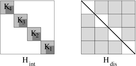
Figure 1: Structures of the interaction and disorder Hamiltonian matrices written in the basis of the PWSDs. The kinetic energy gives a diagonal matrix. We have sketched the structures for 4 subspaces of total momenta ${\bf K}_{1},\ldots,{\bf K}_{4}$. The matrix elements are zero in the white parts. For $H_{int}$, the darker regions corresponds to hopping terms between PWSDs built out from one body states of small momenta $\bf k$ only. In the shaded parts of $H_{int}$ and $H_{W}$, the matrices are sparse.

In Fig. 1, the structure of the Hamiltonian matrix for $N$ spinless fermions is sketched in the basis of the Plane Wave Slater Determinants (PWSDs) $d_{\bf k_{1}}^{\dagger}\ldots d_{\bf k_{N}}^{\dagger}\left|0\right>$. The matrix corresponding to $H_{kin}$ is diagonal. If we order the PWSDs by series of same total momentum ${\bf K}=\sum_{i=1}^{N}{\bf k_{i}}$, the matrix corresponding to $H_{int}$ is block-diagonal, each block being characterized by the same momentum ${\bf K}$. Inside each block, we order the PWSDs by increasing kinetic energy. The matrix elements between PWSDs for which all the components of ${\bf k}$ are small such that $\sin k_{x}\approx k_{x}$ and $\sin k_{y}\approx k_{y}$, are indicated by a darker grey. Moreover, only PWSDs of same ${\bf K}$ having $N-2$ momenta ${\bf k}$ in common out of $N$ can be directly coupled by the two-body interaction. When $N\geq 3$, this means that each block of given ${\bf K}$ is sparse. In contrast, the random matrix due to $H_{W}$ has zero matrix elements inside the diagonal blocks of momenta ${\bf K}$, but gives non zero off-diagonal terms coupling those diagonal blocks. These coupling off-diagonal blocks are even sparser, having non zero terms between PWSDs differing by a single ${\bf k}$ only, out of $N$.

2.3 Lattice factor $r_{s}$

The continuum thermodynamic limit is obtained when the finite size effects due to the finite value of $N$ and the lattice effects due to the finite value of $L$ are negligible. This is clearly out of reach of the Lanczos algorithm. However, for a finite value of $N$, $r_{s}$ remains a scaling parameter when the lattice effects are negligible. In a medium of dielectric constant $\varepsilon$, the strength $U$ of the Coulomb repulsion reads:

$$U=\frac{e^{2}}{\varepsilon s}$$ (14)

while

$$t=\frac{\hbar^{2}}{2m^{*}s^{2}}$$ (15)

is the hopping element between nearest neighbor sites and sets the bandwidth of carriers of effective mass $m^{*}$. Taking $m=m^{*}$ and $\varepsilon=1$, one has in lattice units $1Ry=U^{2}/4t$, $a_{B}=2st/U$ and

$$r_{s}=\frac{a}{a_{B}}=\frac{UL}{2t\sqrt{\pi N}}$$ (16)

for the rydberg, the Bohr radius and the factor $r_{s}$ respectively.

Instead of changing the number $N$ of particles, one can vary $r_{s}$ keeping $N$ fixed and varying $U$, $t$ and $L$, and hence the parameter

$$r_{l}=\frac{UL}{t}=r_{s}\sqrt{4\pi N}.$$ (17)

This amounts to change $r_{s}$ by changing $a_{B}$ instead of $a$. The lattice effects are important fnp either at large values of $U$ (hence large $r_{l}$) for a given $N$, or at large values of $N$ (hence small $r_{s}$) for a given $U$. Hereafter, we use $r_{l}$ or $U$ instead of $r_{s}$ in order to avoid confusion.

3 Persistent current $I$

An Ahronov Bohm flux $\Phi$ is enclosed around the longitudinal $x$-direction as sketched in Fig. 2.

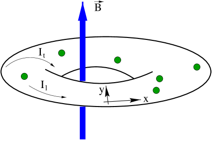
Figure 2: 2d Torus with $N$ electrons enclosing an Aharonov-Bohm flux $\Phi\propto B$

By a gauge transformation, $\Phi$ can be included in the longitudinal BC (antiperiodic BC corresponding to $\Phi=\Phi_{0}/2$ in our convention), while the BC remains always periodic in the transverse $y$-direction. This flux creates persistent currents for a GS of wave-function $\left|\Psi_{0}\right>$ and of energy $E_{0}(\Phi)$:

• At a site ${\bf j}=(j_{x},j_{y})$, the local longitudinal current $j^{l}_{\bf j}(\Phi)$ and the local transverse current $j^{t}_{\bf j}(\Phi)$ read

  $$j^{l}_{\bf j}(\Phi)=2\Im\left<\Psi_{0}\left|c_{\bf j}^{\dagger}c_{(j_{x}+1,j_{y})}e^{2\pi i{\Phi\over L\Phi_{0}}}\right|\Psi_{0}\right>,$$ (18)

  $$j^{t}_{\bf j}(\Phi)=2\Im\left<\Psi_{0}\left|c_{\bf j}^{\dagger}c_{(j_{x},j_{y}+1)}\right|\Psi_{0}\right>$$ (19)

  in units of $\sqrt{t/2m}/s$.

• The total longitudinal current $I_{l}(\Phi)$ enclosing the flux is obtained by summing the local longitudinal currents:

  $$I_{l}(\Phi)=-\frac{\partial E_{0}(\Phi)}{\partial\Phi}=\sum_{j_{y}=1}^{L}j^{l}_{\bf j}={1\over L}\sum_{\bf j}j^{l}_{\bf j}.$$ (20)

  The latter equation comes from the conservation of the current. The total transverse current $I_{t}(\Phi)$ is given by a similar formula using the $j^{t}_{\bf j}\Phi)$.

• The change $\Delta E_{0}(\Phi)$ of the GS energy $E_{0}$ induced by $\Phi$:

  $$\Delta E_{0}(\Phi)=E_{0}(0)-E_{0}(\Phi)$$ (21)

  is a quantity related to $I$ which is simpler to study.

The GS total longitudinal current

$$I_{l}(\Phi)=\frac{2}{L}\Im\sum_{\bf j}\left<\Psi_{0}\left|c_{\bf j}^{\dagger}c_{(j_{x}+1,j_{y})}e^{2\pi i{\Phi\over L\Phi_{0}}}\right|\Psi_{0}\right>$$ (22)

can be expressed in terms of the operators $d_{\vec{k}}^{\dagger}$ ($d_{\vec{k}}$). Hereafter, the $k_{x}$ and $k_{y}$ components are quantized in multiples of $2\pi/L$, and an explicit phase factor $\exp(2\pi\Phi/(\Phi_{0}L))$ is added to the $k_{x}$-components. This gives

$$I_{l}(\Phi)=\frac{2}{L}\Im\sum_{\bf k}e^{i\left(k_{x}+2\pi{\Phi\over L\Phi_{0}}\right)}\left<\Psi_{0}\left|d^{\dagger}_{\bf k}d_{\bf k}\right|\Psi_{0}\right>$$ (23)

for the total longitudinal current and

$$I_{t}(\Phi)=\frac{2}{L}\Im\sum_{\bf k}e^{ik_{y}}\left<\Psi_{0}\left|d^{\dagger}_{\bf k}d_{\bf k}\right|\Psi_{0}\right>$$ (24)

for the total transverse current.

Expressed in terms of its projections $\Psi_{\bf k_{1},\ldots,k_{N}}$ onto the PWSDs $\prod_{n=1}^{N}d_{\bf k_{n}}^{\dagger}\left|0\right>$, the GS reads:

$$\left|\Psi_{0}\right>=\sum_{\bf k_{1},\ldots,k_{N}}\Psi_{\bf k_{1},\ldots,k_{N}}\prod_{n=1}^{N}d_{\bf k_{n}}^{\dagger}\left|0\right>$$ (25)

which gives

$$I_{l}(\Phi) = \frac{2}{L}\sum_{\bf k_{1},\ldots,k_{N}}\left|\Psi_{\bf k_{1}\ldots k_{N}}\right|^{2}\sum_{i=1}^{N}\sin{\left(k_{ix}+2\pi{\Phi\over L\Phi_{0}}\right)}$$

$$I_{t}(\Phi) = \frac{2}{L}\sum_{\bf k_{1},\ldots,k_{N}}\left|\Psi_{\bf k_{1}\ldots k_{N}}\right|^{2}\sum_{i=1}^{N}\sin{k_{iy}}.$$ (26)

4 Relation between $I$ and ${\bf K}$ in the continuum limit and lattice threshold $U^{*}$

As far as the lattice GS occupies small momenta ${\bf k}$, one can approximate the dispersion relation of the lattice model by the parabolic dispersion relation of the continuum limit:

$$2-2\cos k_{i}\approx k_{i}^{2}\ \ \ and\ \ \ \sin k_{i}\approx k_{i}.$$ (27)

In this approximation, the expressions (26) become

$$I_{l}(\Phi) \approx \frac{2}{L}\sum_{\bf k_{1},\ldots,k_{N}}\left|\Psi_{\bf k_{1},\ldots,k_{N}}\right|^{2}\sum_{i=1}^{N}\left(k_{ix}+{2\pi\Phi\over L\Phi_{0}}\right)$$ (28)

$$I_{t}(\Phi) \approx \frac{2}{L}\sum_{\bf k_{1},\ldots,k_{N}}\left|\Psi_{\bf k_{1},\ldots,k_{N}}\right|^{2}\sum_{i=1}^{N}k_{iy}$$ (29)

which give

$$I_{l} = \frac{2}{L}\left(\left<K_{x}\right>+{2\pi N\over L}{\Phi\over\Phi_{0}}\right)$$ (30)

$$I_{t} = \frac{2}{L}\left<K_{y}\right>,$$ (31)

where $\left<K_{x,y}\right>=\sum_{\bf k_{1},\ldots,k_{N}}\left(\sum_{i=1}^{N}k_{i,x,y}\right)\left|\Psi_{\bf k_{1},\ldots,k_{N}}\right|^{2}$.

This proves an important theorem which was known in one dimension and numerically checked muller-groeling ; krive ; burmeister in two dimensions: the GS persistent current $I$ is independent of the interaction strength $U$ in the continuum limit of a non-disordered lattice model of arbitrary dimensions. Moreover, this provides one criterion (criterion 2 of Ref. fnp ) for obtaining the lattice threshold $U^{*}$. We have shown that $I$ is proportional to ${\bf K}$ when the momenta ${\bf k}$ occupied by the GS are small, allowing to use the approximation (27). The invariance of $I$ is a direct consequence of the invariance of ${\bf K}$. When $U=W=0$, the approximations (27) require small filling factors $N/L^{2}$. If one turns on $U$ for $W=0$ and a small filling factor, $I\propto{\bf K}$ remains independent of $U$ when $U$ is smaller than the threshold $U^{*}$. When $U>U^{*}$, the GS of a non-disordered lattice begins to occupy, inside the same subspace of total momentum ${\bf K}$, large one particle momenta ${\bf k}$, and the relation between $I$ and ${\bf K}$ ceases to be valid. Without disorder, ${\bf K}$ is always conserved, and $I$ remains independent of $U$ as far as $I\propto{\bf K}$. The breakdown of the invariance of $I$ is a consequence of a localization-delocalization crossover induced by $U$ in momentum space. For a fixed value of $t$, this crossover can be induced by $U$ inside a subspace of given total momentum ${\bf K}$, by $W$ among subspaces of different ${\bf K}$, or by the combined role of $U$ and $W$. The regime where ${\bf K}$ is conserved defines the ballistic many body regime.

5 Overview of the non disordered case for $N=3$

Before considering the case where random potentials are included, it is useful to summarize what we know when there is no disorder. Let us review a few published np ; fnp and unpublished results based on a study of the case $N=3$.

5.1 Continuum Wigner molecule above $U^{W}$
($r_{s}>r_{s}^{W}\approx 50$)

On a continuum $D\times D$ square with periodic BCs, the Coulomb repulsion with the taken $2d$ metric reads

$$V({\bf r})={e^{2}\pi\over D\sqrt{\sin^{2}{r_{x}\pi\over D}+\sin^{2}{r_{y}\pi\over D}}}.$$ (32)

The GS center of mass is delocalized. When the density $N/D^{2}$ is small enough, the spacings $d$ between the particles are large and one obtains a Wigner molecule, which is in the continuum limit if the fluctuations of $d$ are also larger than $s$. For a given center of mass, to put the particle on the sites ${\bf r}_{1}=(0,0)$, ${\bf r}_{2}=(D/3,D/3)$ and ${\bf r}_{3}=(-D/3,-D/3)$ yields for the Coulomb energy a minimum value:

$$E_{Coul}=\frac{\sqrt{6}e^{2}\pi}{D}.$$ (33)

For a large $D$, one can expand the pair-potential around the equilibrium inter-particle spacing ${\bf r}_{0}=(D/3,D/3)$ up to the second order to get harmonic oscillations around the equilibrium positions. The Hamiltonian $H_{c}\approx E_{Coul}+H_{harm}$, where the harmonic part reads:

$$H_{harm}={1\over 2m}\sum_{i=1}^{3}{\bf p}_{i}^{2}+{\vec{X}}{\hat{M}}{\vec{X}}.$$ (34)

The vector ${\vec{X}}=(x_{1},y_{1},x_{2},y_{2},x_{3},y_{3})$ describes the motions of the molecule around equilibrium. The $6\times 6$ matrix ${\hat{M}}$ is given by:

$${\hat{M}}=\left(\matrix{2A&2B&-A&-B&-A&-B\cr 2B&2A&-B&-A&-B&-A\cr-A&-B&2A&2B&-A&-B\cr-B&-A&2B&2A&-B&-A\cr-A&-B&-A&-B&2A&2B\cr-B&-A&-B&-A&2B&2A}\right).$$ (35)

where

$$A={7\sqrt{6}\over 72}{e^{2}\pi\over D^{3}}$$ (36)

and $B=3A/7$. Diagonalizing ${\hat{M}}$, one obtains the normal modes, while the eigenvalues of ${\hat{M}}$ give their frequencies.

One obtains two eigenvectors ${\vec{\chi}_{1}}$ and ${\vec{\chi}_{2}}$ of eigenvalue $0$, which corresponds to the translation of the center of mass of the molecule, two other eigenvectors ${\vec{\chi}_{3}}$ and ${\vec{\chi}_{4}}$ of eigenvalue $10B$, which corresponds to the longitudinal mode, while the two last eigenvectors ${\vec{\chi}_{5}}$ and ${\vec{\chi}_{6}}$ of eigenvalue $4B$ correspond to the transverse mode. The expressions of eigenvectors ${\vec{\chi}_{i}}$ are given in Ref. fnp .

Using these normal coordinates, the Hamiltonian (34) becomes a decoupled sum of four harmonic oscillators:

$$H_{harm}-{\hbar^{2}\over 2m}\sum_{\alpha=1}^{6}{\partial^{2}\over\partial\chi_{\alpha}^{2}}=10B(\chi_{3}^{2}+\chi_{4}^{2})+4B(\chi_{5}^{2}+\chi_{6}^{2}),$$ (37)

Without disorder, the interaction can only couple states of same total momentum ${\bf K}$. Inside a subspace of a total momentum ${\bf K}$, the wave functions can be factorized as

$$\Psi(\chi_{1},\dots,\chi_{6})=\Psi^{\bf K}_{cm}(\chi_{1},\chi_{2})\Psi^{n_{3},\dots,n_{6}}_{rel}(\chi_{3},\dots,\chi_{6}).$$ (38)

The kinetic energy associated to the motion of the center mass reads:

$$E_{cm}({\bf K})=-{\hbar^{2}\over 2Nm}{\bf K}^{2}.$$ (39)

The wave-function $\Psi^{n_{3}=0,\dots,n_{6}=0}(\chi_{3},\dots,\chi_{6})$ corresponding to the relative motions can be factorized as:

$$\Psi^{n_{3}=0,\dots,n_{6}=0}_{rel}=\varphi_{0L}(\chi_{3})\varphi_{0L}(\chi_{4})\varphi_{0T}(\chi_{5})\varphi_{0T}(\chi_{6})$$ (40)

for the ground state ($n_{3}=0,\dots,n_{6}=0$) of momentum ${\bf K}$. $L,T$ refer to the transverse and longitudinal modes and $\varphi_{0}$ is the GS of an harmonic oscillator:

$$\varphi_{0}(x)={1\over l_{\omega}^{1/2}\pi^{1/4}}\exp-\frac{x^{2}}{2l_{\omega}^{2}},$$ (41)

of characteristic length:

$$l_{\omega}=\left(\frac{\hbar^{2}}{m^{2}\omega^{2}}\right)^{1/4}.$$ (42)

For the expanded pair potentials, the GS energy $E_{0}({\bf K})$ inside a subspace of momentum ${\bf K}$ becomes

$$E_{0}({\bf K})=E_{Coul}+E_{cm}({\bf K})+\hbar(\omega_{T}+\omega_{L});$$ (43)

where

$$\omega_{L}=\sqrt{\frac{20B}{m}}\ \ ,\ \omega_{T}=\sqrt{\frac{8B}{m}}.$$ (44)

In lattice units, one gets:

$$E_{0}({\bf K})=E_{Coul}+E_{cm}({\bf K})+E_{rel,0},$$ (45)

where $E_{rel}(n_{3}=0,\dots,n_{6}=0)=E_{rel,0}$.

$$E_{cm}({\bf K}) = \frac{t}{N}{\bf K}^{2}$$ (46)

$$E_{rel,0} = \frac{\sqrt{6}\pi U}{L}+(\sqrt{5}+\sqrt{2})\sqrt{\sqrt{6}\pi^{3}\over 3}\sqrt{Ut\over L^{3}}.$$ (47)

$E_{0}({\bf K})$ depends on ${\bf K}$ only through $E_{cm}({\bf K})$, while $E_{Coul}$ and the transverse and longitudinal modes remain independent of ${\bf K}$. This is still the case if one goes beyond the harmonic approximation for the pair potentials, including anharmonic corrections. The only approximation which we have done is to assume that the relative motions are small compared to $D$. Thus the GS relative wave functions $\Psi^{n_{3}=0,\dots,n_{6}=0}_{rel}(\chi_{3},\dots,\chi_{6})$ and $E_{rel}(n_{3}=0,\dots,n_{6}=0)$ are approximated by the solutions of an unbounded $2d$ system, while the wave functions of the center of mass $\Psi^{\bf K}_{cm}(\chi_{1},\chi_{2})$ and $E_{cm}({\bf K})$ correspond to a bounded $2d$ system. The assumed $2d$ harmonic oscillations make sense only if the Wigner molecule is rigid enough for making negligible the boundary effects upon the relative motions.

5.2 Supersolid molecule below $U^{W}$
($r_{s}^{F}<r_{s}<r_{s}^{W}$)

To determine the values of $r_{s}$ where the GS energy is described by Eq (45), we plot in Fig. 3 the GS energies $E_{0}({\bf K})-E_{cm}({\bf K})-E_{Coul}$ as a function of $r_{s}$, for a size $L=18$ and different subspaces of momentum ${\bf K}$. $E_{Coul}=\sqrt{6}\pi U/L$ when $L/3$ is integer.

Figure 3: $W=0$, $L=18$ and $N=3$: The GS-energies $E_{0}({\bf K})-E_{cm}({\bf K})-E_{Coul}$ for different total momenta ${\bf K}$ as a function of $r_{s}$. The arrow shows $r_{s}^{W}\approx 50$ above which the behavior is given by Eq 45 (solid line $0.139\sqrt{r_{s}}$) up to the lattice threshold $r_{s}^{*}$.

The solid line ($0.139\sqrt{r_{s}}$) gives the behavior implied by the continuum harmonic expansion (Eq 45) with unbounded relative motions. One can see that this theory is accurate for $r_{s}^{W}<r_{s}<r_{s}^{*}$. Above $r_{s}^{W}\approx 50$, the relative motions become localized and coincide to unbounded harmonic vibrations. Below $r_{s}^{W}$, the behavior is more complicated. On one side, the $E_{0}({\bf K})$ are roughly described above $r_{s}^{F}\approx 10$ by the expansion (45) valid for a continuum solid molecule. On the other side, the relative motions depend on ${\bf K}$, a dependence which cannot exist unless the relative motions are extended over a scale of the order of the system size $D=Ls$. Large zero-point motions are expected in a supersolid. For $N=3$, we have shown that there is regime where there is a floppy Wigner molecule, though the relative motions depends on the quantization of ${\bf K}$ and hence on the BCs. This intermediate “supersolid” regime was noted in Ref. np using another $2d$ metric for $L=6$, a limit where the lattice effects play a role. Our results for a Wigner molecule describable by a continuum theory when $L=18$ gives further support to the existence of an intermediate regime for $r_{s}^{F}<r_{s}<r_{s}^{W}$ which is not a lattice effect. Hereafter, we use the word “supersolid” to refer to this regime.

5.3 Lattice regime above $U^{*}(L)$
($r_{l}>r_{l}^{*}(L)$)

The GS energy of the lattice model (Hamiltonian 3) is also not described by the continuum expansion (45) above the lattice threshold $r_{l}^{*}(L)$. Three equivalent criteria were introduced in Ref. fnp for giving $r_{l}^{*}(L)$. One was based on the breakdown of the invariance of $I$ discussed in section 4. Let us introduce a fourth criterion which gives a similar answer: the lattice spacing $s$ becomes relevant when the size $l_{\omega}$ of the harmonic oscillations becomes of the order of the lattice spacing $s$. The longitudinal modes giving the smallest scale, the criterion reads

$$l_{\omega_{L}}=\left(\frac{\hbar^{2}}{m^{2}{\omega}_{L}^{2}}\right)^{1/4}\approx s,$$ (48)

giving $r_{l}^{*}(L)\approx(2\sqrt{6})/(5\pi)L^{4}$ or

$$\frac{U^{*}(L)}{t}\approx\frac{2\sqrt{6}}{5\pi}L^{3}.$$ (49)

When $U>U^{*}(L)$ ($r_{l}>r_{l}^{*}(L)$), the lattice model exhibits a different behavior than its continuum limit and $r_{s}$ ceases to be a scaling parameter. This difference is shown in Fig. 4, where one can see the universal scaling regime below $r_{l}^{*}(L)$ and the non universal lattice behaviors above $r_{l}^{*}(L)$.

To show scaling when the GSs of different total momenta ${\bf K}$ correspond to a rigid molecule with ${\bf K}$-independent harmonic oscillations and a ${\bf K}$-dependent translation of the center of mass, we use the dimensionless quantum correction $F_{0}({\bf K},r_{l})$ to the classical electrostatic energy:

$$F_{0}({\bf K},r_{l})=\frac{E_{0}({\bf K},r_{l})-E_{cm}({\bf K})-E_{Coul}}{E_{0}({\bf K}=0,U=0)}.$$ (50)

$F_{0}({\bf K},r_{l})$ is shown in Fig. 4 as a function of $r_{l}=UL/t$ for different momenta ${\bf K}$ and $N=3$. One can see that the data obtained for $L=9$ and $18$ are on the same universal curve below $r_{l}^{*}(L)$, the curve depending on ${\bf K}$ below a value $r_{l}^{W}$ corresponding to $r_{s}^{W}\approx 50$. The universal ${\bf K}$-independent scaling curve $0.2326\sqrt{r_{l}}$ is obtained assuming that $E_{0}({\bf K}=0,U=0)\approx 8\pi^{2}t/L^{2}$ as in the continuum limit:

$$F_{0} = {\sqrt{5}+\sqrt{2}\over 8\pi^{2}}\sqrt{\sqrt{6}\pi^{3}\over 3}\sqrt{UL\over t}$$ (51)

$$= {\sqrt{5}+\sqrt{2}\over\sqrt{96}}\left({18\over\pi}\right)^{1/4}\sqrt{r_{s}}$$

$$= 0.5764\sqrt{r_{s}}=0.2326\sqrt{r_{l}}.$$

$F_{0}$ saturates above $r_{l}^{*}(L)$ to a value $4Nt/(8\pi^{2}t/L^{2})$ which is independent of $U$.

Figure 4: $W=0$, $N=3$: The dimensionless GS-energies $F_{0}$ for different total momenta ${\bf K}$ as a function of $r_{l}=UL/t$ for $L=9$ and $L=18$. The solid line $0.2326\sqrt{r_{l}}$ comes from Eq (51).

6 Effects of a weak disorder in the lattice regime of an electron solid

Figure 5: Sketches of the hopping processes characterizing the three lattice regimes of a very weakly disordered lattice when $U>U^{*}$ for $L=6$ and $N=3$. From left to right: Ballistic Wigner molecule (BWM) when $U^{*}<U<U_{stripe}$; Coulomb Guided Stripe of Current (CGSC) when $U_{stripe}<U<U_{loc}$ and one particle motion out of a Localized Wigner Molecule (LWM) above $U_{loc}$.

Without interaction ($U=0$) one has three regimes (ballistic, diffusive and localized) as $W$ increases. Assuming Drude formula and Born approximation, the dimensionless conductance $g$ reads walker :

$$g\approx\frac{k_{F}l}{2}\approx 96\pi\frac{N}{L^{2}}\left(\frac{t}{W}\right)^{2}.$$ (52)

For a Fermi momentum $k_{F}\approx\sqrt{4\pi N}/(Ls)^{2}$, the elastic mean free path $l$ becomes

$$l\approx\frac{96\sqrt{\pi}N}{L}\left(\frac{t}{W}\right)^{2}s.$$ (53)

If $U=0$, $N=3$, $L\approx 6-9$, this gives a ballistic motion when $W/t\approx 0.01-0.1$, a diffusive motion when $W/t\approx 1$, and strong Anderson localization for $W/t\approx 10-20$.

Let us first study the effect of a weak disorder in the simple lattice regime where the three particles form an electron solid (Wigner molecule). Since $r_{l}$ becomes an irrelevant parameter above $r_{l}^{*}$, we simply use the parameter $U$, $U^{*}$ being the interaction strength corresponding to $r_{l}^{*}(L)$ for the used values of $L$ and $t$. For $U>U^{*}$, the low energy physics of the $N$-body problem can be described by an effective one particle problem. For $N=3$ and $L/3$ integer, the Wigner molecule is oriented along one of the two diagonals of the square lattice. The average interparticle spacing $\left<d\right>=(\pm L/3,\pm L/3)$ and the fluctuations of $d$ are smaller than $s$ above $U^{*}$. Taking $t=1$, a fixed value of $L$ and a weak value of $W$, one gets three lattice regimes when one increases $U$ above $U^{*}$, characterized by three different lattice perturbation expansions. First, there is a Ballistic Wigner Molecule (BWM) on a scale $L$ smaller than the elastic mean free path $l_{cm}$ characterizing the motion of the center of mass. On this small scale, the disorder can be neglected, the motion of the center of mass remains ballistic and can be described by a non-random single particle lattice model with an effective nearest neighbor hopping term $t_{eff}\propto t^{N}/U^{N-1}$. Above an interaction $U_{stripe}>U^{*}$, the effects of disorder become relevant and must be included in the effective single particle model. This gives a new regime where the interplay between disorder and electronic correlations leads to a Coulomb Guided Stripe of Current (CGSC), since the current $I$ flows along the axis of the Wigner molecule. Eventually, the effective model breaks down when $U$ exceeds a large threshold $U_{loc}>U_{stripe}>U^{*}$, and we have the perturbative regime analyzed in refs. efros ; sw for a localized Wigner molecule (LWM). While the motion induced by $\Phi$ is along the shortest paths enclosing $\Phi$ in the BWM and in the LWM regimes, the motion in the intermediate CGSC regime uses a longer path of smaller electrostatic cost.

In Fig. 5, we have sketched the different hopping processes characterizing these three regimes when $L=6$. The left figure corresponds to a Ballistic Wigner molecule (BWM). The middle figure describes the Coulomb Guided Stripe of Current (CGSC) induced by the interplay between disorder and electronic correlations. The right figure shows a Localized Wigner Molecule (LWM) carrying exponentially small one particle currents.

6.1 Lattice regime for a Ballistic Wigner Molecule

When $L$ is smaller than the elastic mean path $l_{cm}$ of the center of mass of the Wigner molecule, ${\bf K}$ does not vary and one can consider a subspace of total momentum ${\bf K}$. Assuming $L/3$ integer and $t/U\rightarrow 0$, the GS reads

$$\left|\Psi_{0}({\bf K})\right>=A\sum_{\bf j}e^{i{\bf K\cdot j}}C^{\dagger}_{\bf j}\left|0\right>,$$ (54)

where

$$C^{\dagger}_{\bf j}=c^{\dagger}_{\bf j}c^{\dagger}_{{\bf j}+(L/3,L/3)}c^{\dagger}_{{\bf j}+(2L/3,2L/3)}$$ (55)

and $A$ is a normalization constant. When $t=0$, we have $2L^{2}/3$ configurations $C^{\dagger}_{\bf j}\left|0\right>$ of identical Coulomb energy $E_{Coul}$. Without disorder, this large degeneracy is removed by a hopping term $t_{eff}\propto t^{3}/U^{2}$ coupling two nearest neighbor configurations $C^{\dagger}_{\bf j}\left|0\right>$ and $C^{\dagger}_{\bf j^{\prime}}\left|0\right>$, as indicated in Fig. 5 left. At this order, one gets an effective one particle $L/3\times L$ lattice model described by

$$H_{eff}(W=0)=4Nt+E_{Coul}-t_{eff}\sum_{\left<{\bf j,j^{\prime}}\right>}C^{\dagger}_{\bf j}C_{\bf j^{\prime}}.$$ (56)

where the effective hopping term reads

$$t_{eff}=\sum_{\{P\}}\frac{t^{N}}{\prod_{\gamma}\left(E_{Coul}-E_{P_{\gamma}}\right)},$$ (57)

$P$ labeling a series of intermediate configurations coupling ${\bf j}$ and ${\bf j^{\prime}}$ of Coulomb energy $E_{P_{\gamma}}$. This gives

$$t_{eff}\sim{t^{N}\over U^{N-1}}L^{3N-3},$$ (58)

and for $N=3$

$$t_{eff}=6{t^{3}\over\left({7\sqrt{6}\over 36}{U\pi\over L^{3}}\right)^{2}}.$$ (59)

Including the flux in the longitudinal hopping terms $t_{eff}\exp\left(i2\pi N\Phi/\Phi_{0}L\right)$, one gets for the change of the GS energy

$$\Delta E_{0}\left(\Phi,{\bf K}\right)=2t_{eff}\left(\cos(K_{x}+\frac{2\pi N\Phi}{\Phi_{0}L})-\cos K_{x}\right).$$ (60)

In Fig. 6 as in the following ones, the maps of local currents characterizing a disordered sample and the corresponding site occupation numbers $n_{\bf j}^{0}$ given by

$$n_{\bf j}^{0}=\left<\Psi_{0}(U)\left|c^{\dagger}_{\bf j}c_{\bf j}\right|\Psi_{0}(U)\right>$$ (61)

are shown using the same convention: the arrows between neighboring sites give the local currents, the largest local current found in the sample is shown by an arrow of length $s$, while $n_{\bf j}^{0}=1$ is shown by a disk of diameter $s$. A small value $\Phi=0.05\Phi_{0}$ is used for driving the persistent currents.

In Fig. 6, the map of local currents are given for a weakly disordered sample ($W=0.01$ and $t=1$) with an interaction strength $U=300$ above $U^{*}$ and the corresponding site occupation numbers $n_{\bf j}^{0}$. The map of currents and the density exhibit an almost perfect translational invariance in this ballistic regime and gives an illustration of the BWM motion characterized by $t_{eff}$.

Figure 6: Ballistic translation of a Wigner Molecule in the lattice regime (BWM regime), obtained in a disordered sample with $N=3$, $L=9$, $W=0.01$, $t=1$ and $U=300$. Left figure: map of currents for $\Phi=0.05\Phi_{0}$. Right figure: corresponding site occupation numbers $n_{\bf j}^{0}$.

6.2 Lattice regime for a Coulomb Guided Stripe of Current

As one continues to increase $U$, the effect of disorder cannot be ignored and the Wigner molecule finishes to be pinned in the GS configuration $C^{\dagger}_{\bf j}\left|0\right>$ of minimum Coulomb energy for which $\sum_{\bf j}\epsilon_{\bf j}$ is also minimum. As one can see in Fig. 7 (right), a complete localization of the center of mass of the rigid molecule is achieved for a disordered sample with $W=t=1$ and $U=1000$. The GS probability to occupy a site is almost zero outside three sites where $C^{\dagger}_{\bf j}\left|0\right>$ has a minimum energy. It is likely that this complete localization is obtained after a small diffusive regime. In this pinned regime, two competing motions are now relevant for enclosing the flux, which are sketched in Fig. 5 (middle and right). The CGSC motion (Fig. 5 middle) is larger when $U_{stripe}<U<U_{loc}$ while the LWM motion (Fig. 5 right) dominates the longitudinal motion when $U_{loc}<U$. Let us first study the CGSC motion. The effect of disorder can be included by adding random site potentials $W\omega_{\bf j}$ to the effective one particle model (56):

$$H_{eff}(W)=H_{eff}(W=0)+W\sum_{\bf j}\omega_{\bf j}C^{\dagger}_{\bf j}C_{\bf j},$$ (62)

where $\omega_{\bf j}=\epsilon_{\bf j}+\epsilon_{{\bf j}+(L/3,L/3)}+\epsilon_{{\bf j}-(L/3,L/3)}$.

Assuming the Hamiltonian (62), the GS flux dependence is obtained at the order $2L/3$ of an expansion in powers of $t_{eff}/W$, corresponding to the $(L/3,L/3)$-translation shown in Fig. 5 middle. One gets for the GS energy change

$$\Delta E_{0}\left(\Phi\right) \propto \frac{t_{eff}^{2L/3}\cos\left(2\pi\Phi/\Phi_{0}\right)}{{{\sqrt{N}}W}^{2L/3-1}}$$ (63)

$$\propto \frac{t^{2L}L^{4L}\cos\left(2\pi\Phi/\Phi_{0}\right)}{W^{2L/3-1}U^{4L/3}},$$ (64)

which gives for the two sizes $L$ which we have studied

$$\Delta E_{0}\left(L=6,\Phi\right) \propto \frac{t^{12}}{W^{3}U^{8}}\cos\left(2\pi\Phi/\Phi_{0}\right)$$ (65)

$$\Delta E_{0}\left(L=9,\Phi\right) \propto \frac{t^{18}}{W^{5}U^{12}}\cos\left(2\pi\Phi/\Phi_{0}\right)$$ (66)

respectively.

The current $I$ forms a stripe which follows the axis of the pinned Wigner molecule for enclosing the flux. The path is longer than the shortest path, but it uses intermediate configurations of minimum Coulomb energy. An illustration of such a stripe is given in Fig. 7 (left), obtained using a disordered sample where $W=t=1$ and $U=1000$: the pinned Wigner molecule carries in the CGSC regime a current of components $I_{l}=I_{t}$, in contrast to the BWM and LWM regimes where $I_{t}$ is negligible compared to $I_{l}$.

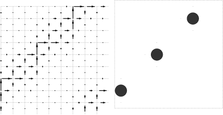
Figure 7: Coulomb Guided Stripe of Current (CGSC) in the lattice regime, obtained in a disordered sample with $N=3$, $L=9$, $W=t=1$ and $U=1000$. Left figure: map of currents for $\Phi=0.05\Phi_{0}$. Right figure: corresponding site occupation numbers $n_{\bf j}^{0}$.

6.3 Lattice regime for a Localized Wigner Molecule

When $U$ becomes very large, the previous CGSC remains and gives the transverse current $I_{t}$, but the main contribution to $I_{l}$ is no longer given by the effective Hamiltonian (62). This is because one particle hops, using $L-1$ intermediate states of high Coulomb energy become more advantageous than the correlated effective hopping using $2L-1$ states of smaller Coulomb energy. For $N=3$, this corresponds to one particle hops along the shortest path inclosing the flux (see Fig. 5 right). To numerically get this regime for a very weak disorder and $L=9$ requires a very large value of $U/t$, where the numerical results become inaccurate. Nevertheless, an illustration of this regime using a sample with a large disorder ($W/t=20$) is given for $U/t=1000$ in Fig. 8, with the corresponding GS occupation numbers.

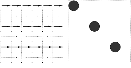
Figure 8: One particle motions out of a Localized Wigner Molecule (LWM) in the lattice regime: Disordered sample with $N=3$, $L=9$, $t=1$, $W=20$ and $U=1000$. Left figure: map of currents for $\Phi=0.05\Phi_{0}$. Right figure: corresponding site occupation numbers $n_{\bf j}^{0}$.

The GS energy change $\Delta E_{0}\left(\Phi\right)$ reads:

$$\Delta E_{0}\left(\Phi\right)\propto\frac{t^{L}L^{3L-3}}{U^{L-1}}\cos\left(2\pi\Phi/\Phi_{0}\right)$$ (67)

which gives for the two sizes $L$ which we have studied

$$\Delta E_{0}\left(L=6,\Phi\right) \propto \frac{t^{6}}{U^{5}}\cos\left(2\pi\Phi/\Phi_{0}\right)$$ (68)

$$\Delta E_{0}\left(L=9,\Phi\right) \propto \frac{t^{9}}{U^{8}}\cos\left(2\pi\Phi/\Phi_{0}\right)$$ (69)

respectively.

6.4 Crossovers between the different lattice regimes

To obtain the threshold values where a crossover between different lattice regimes occurs, we compare the GS energy changes $\Delta E_{0}\left(\Phi\right)$ of the different lattice regimes (Eqs. 60, 64 and 67).

Increasing $W/t$ for a ratio $U/t>U^{*}/t$, the BWM-CGSC crossover takes place when $W$ reaches a threshold value $W_{stripe}\approx t_{eff}$. This gives:

$$\frac{W_{stripe}}{t}\propto\left(\frac{t}{U}\right)^{2}L^{6}.$$ (70)

The CGSC-LWM crossover takes place when $W/t$ reaches a second threshold

$$\frac{W_{loc}}{t}\propto\left(\frac{t}{U}\right)^{\frac{L+3}{2L-3}}L^{\frac{3L+9}{2L-3}}$$ (71)

If one increases $U/t$ above $U^{*}/t$ for a given ratio $W/t$, the BWM-CGSC crossover occurs when $U/t$ becomes of the order of

$$\frac{U_{stripe}}{t}\propto\left(\frac{t}{W}\right)^{1/2}L^{3},$$ (72)

followed by the CGSC-LWM crossover when $U/t$ reaches

$$\frac{U_{loc}}{t}\propto\left(\frac{t}{W}\right)^{\frac{2L-3}{L+3}}L^{\frac{3L+9}{L+3}}.$$ (73)

Figure 9: $L=6$ and $t=1$: Amplitude $|I_{l}(\Phi=0.05\Phi_{0})|$ of the total longitudinal current as a function of $U$ for a disordered sample with increasing values of $W$. The thick solid lines give the expected lattice decays.

Figure 10: $L=9$ and $t=1$: Amplitude $|I_{l}(\Phi=0.05\Phi_{0})|$ of the total longitudinal current as a function of $U$ for a disordered sample with increasing values of $W$. The thick solid lines give the expected lattice decays.

7 Numerical results for $N=3$ particles.

The study of different samples confirms the dependences of the effective hopping terms predicted for the three lattice regimes as a function of the lattice parameters $U$, $W$ and $t$ in the expected ranges of parameters. We show numerical results for the total currents $I_{l}$ and $I_{t}$, and their ratios $I_{t}/I_{l}$ obtained using disordered samples, fixing two parameters ($U$, $W$ or $t$) and varying the third, when a small flux $\Phi=0.05\Phi_{0}$ is enclosed. We give the typical behavior obtained using a single sample, without ensemble average. The sample to sample fluctuations are negligible for weak disorders, and can be more important when $W$ becomes large.

7.1 Persistent currents as a function of $U$

In Figs. 9 and 10, the amplitude of the total longitudinal current $|I_{l}|$ is shown as a function of $U$ for $t=1$ and various values of $W$, for $L=6$ and $9$ respectively. The power laws with the predicted exponents characterize the decay of the currents ($U^{-2},U^{-4L/3}$ and $U^{1-L}$) in the three expected lattice regimes.

Figure 11: $L=6$ and $t=1$: Ratio $I_{t}/I_{l}$ for $\Phi=0.05\Phi_{0})$ as a function of $U$ for increasing values of $W$.

Figure 12: $L=9$ and $t=1$: Ratio $I_{t}/I_{l}$ for $\Phi=0.05\Phi_{0}$ as a function of $U$ and increasing values of $W$.

In Figs. 11 and 12, the ratio $|I_{t}/I_{l}|$ is given as a function of $U$. Since the stripe of current characterizing the CGSC-regime yields a ratio $|I_{t}/I_{l}|=1$, one can see on those figures the values of $U$ where the CGSC-regime takes place. For small values of $U$ which are below the lattice threshold $U^{*}$, one can see in Figs. 9 and 10 that $|I_{l}|$ and $|I_{t}|$ are essentially independent of $U$, excepted around a value $U_{lc}$ where an avoided level crossing occurs. The value of $U_{lc}$ depends on $W$ and $t$ and exhibits small sample to sample fluctuations. This avoided crossing yields a change of the sign of $I_{l}$, a sharp drop of $|I_{l}|$ and a singularity in $|I_{t}/I_{l}|$ which can be seen in Figs. 11 and 12. The continuum behaviors taking place when $U<U^{*}$, where $I_{l}$ and $I_{t}$ are essentially independent of $U$ instead of exhibiting the lattice decays while $|I_{t}/I_{l}|\approx 1$, are studied in section 9.

7.2 Persistent currents as a function of $W$

Figure 13: $L=6$ and $t=1$: Amplitudes $|I_{l}|$ (indicated by a line with a symbol) and $|I_{t}|$ (indicated by a line without symbol) of the total longitudinal and transverse currents as a function of $W$. The data are obtained using a disordered sample with $\Phi=0.05\Phi_{0}$. The symbols and lines corresponding to different values of $U$ are defined in the figure. The thick solid lines give the $W^{-3},W^{-1},W^{1}$ and $W^{2}$ decays respectively.

Figure 14: $L=9$ and $t=1$: Amplitudes $I_{l}$ (indicated by a line with a symbol) and $I_{t}$ (indicated by a line without symbol) as a function of $W$. The studied values of $U$ are represented as in Fig.13. The thick solid lines give the $W^{-5},W^{-1}$ and $W^{2}$ decays respectively.

Figs. 13 and 14 show for $L=6$ and $9$ respectively how the amplitudes $|I_{l}|$ (indicated by lines with symbols) and $|I_{t}|$ (indicated by the same lines without symbol) vary as a function of $W$ for $t=1$ and various values of $U$. When $U$ is large ($U=100-1000$), one can see the expected lattice behaviors: the CGSC-decay $I_{l}\propto W^{-(2L/3-1)}$ for $W_{stripe}<W<W_{loc}$ followed above $W_{loc}$ by the LWM-regime where $I_{l}$ saturates to a small value independent of $W$. When $U$ is smaller ($U=1-10$), $I_{l}$ is first almost independent of $W$, before decaying as $W^{-1}$ when $1<W<10$ for $L=6$ and $9$.

The transverse current $I_{t}$ begins to increase as a function of $W$ from the zero value characterizing the limit $W=0$. This increase of $I_{t}$ takes place for the values of $W$ where $I_{l}$ is roughly independent of $W$. This increase goes as $W^{2}$ for large interactions ($U=100-1000$) and as $W$ for small interactions ($U=1-10$), as underlined in Fig.13. These two different powers can be explained by a perturbative expansion in powers of $W$. When $W=0$, GSs of different total momenta ${\bf K}$ are degenerate when $U$ is small and $I_{t}\propto W$. As $U$ increases, there is a level crossing for $W=0$ above which there is a non-degenerate GS of momentum ${\bf K}=0$ and $I_{t}\propto W^{2}$ when $U$ is large. The increase of $I_{t}$ is followed by a regime where $I_{t}\approx I_{l}$ when $L=6$ or exhibits the same decays ($W^{-1}$ or $W^{-(2L/3-1})$) than $I_{l}$ when $L=9$. For large $U$ and above $W_{loc}$, $I_{t}$ continues to decay as in the lattice CGSC-regime ($I_{t}\propto W^{-(2L/3-1)}$) while $I_{l}$ saturates to a $W$-independent value.

7.3 Persistent currents as a function of $t$

Figure 15: $L=6$ and $W=1$: Amplitudes $|I_{l}|$ (lines with symbols) and $|I_{t}|$ (lines without symbol) as a function of $t$, obtained using a disordered sample with increasing values of $U$ and $\Phi=0.05\Phi_{0}$. The thick solid lines give the expected lattice behaviors.

Figure 16: $L=9$ and $W=1$: Amplitudes $|I_{l}|$ (line with symbols) and $|I_{t}|$ (line without symbol) as a function of $t$, obtained using a disordered sample with increasing values of $U$ and $\Phi=0.05\Phi_{0}$. The thick solid lines give the expected lattice behaviors.

In Figs. 15 and 16, the amplitudes $|I_{l}|$ and $|I_{t}|$ are shown as a function of $t$ for $W=1$ and various values of $U$, using disordered samples of size $L=6$ and $9$ respectively. The power laws shown by thick lines give the decay of the currents $t^{L},t^{2L}$ for $L=6$ and $9$ respectively, as expected for lattice regimes ($t<t^{*}$) with $W=1$. The $t^{3}$-behavior expected in the BWM-regime requires a smaller disorder to be observed. For $t>t^{*}$, the behaviors are similar to those observed for $t=1$ and $U<U^{*}$. In the lattice LWM regime ($t\rightarrow 0$), one can see that $|I_{t}|$ continues to exhibit the lattice CGSC-behavior $\propto t^{2L}$ while $|I_{l}|\propto t^{L}$ becomes much larger.

8 Continuum-Lattice crossovers with disorder

We have shown in section 4 that $I\propto\left<{\bf K}\right>$ unless the GS begins to occupy states of high momenta ${\bf k}$. Therefore, the breakdown of the interaction-invariance of $I$ is a consequence of a localization-delocalization transition induced by $U$ or $W$ in momentum space, unless one has a level crossing. Without disorder, a jump in the GS total momentum ${\bf K}$ can be induced by level crossings between GSs of different ${\bf K}$. In the presence of disorder, these level crossings become avoided level crossings. We discuss in the following sub-section how avoided level crossings limit the interaction-invariance of $I$, outside the lattice regimes where the relation $I\propto\left<{\bf K}\right>$ is broken.

8.1 Level crossings below $r_{s}^{W}$ and momentum conservation

When $W=0$, ${\bf K}$ is conserved and one can follow the GS of given ${\bf K}$ as a function of $U$. When $U=0$, the GS momentum is ${\bf K}=0$ only if the Fermi shell is full. For a square lattice, this corresponds to $N=1,5,9,\ldots$. For $U^{W}<U<U^{*}$, the GS is a Wigner molecule with harmonic oscillations and a delocalized center of mass. This is what we have shown for $N=3$ in section. 5. The GS energy

$$E_{0}({\bf K},r_{s})\approx E_{cm}({\bf K})+E_{rel}(r_{s})+E_{coul}$$ (74)

depends on ${\bf K}$ via the motion of the center of mass only. In this continuum Wigner regime, the kinetic energy of the center of mass is minimum for ${\bf K}=0$. So for $N=1,5,9,\ldots$, the GS remains in the sub-space of ${\bf K}=0$ when $U$ varies and does not exhibit level crossings between GSs of different ${\bf K}$. For $N=3$, this is different, because the GS momentum ${\bf K}\neq 0$ at $U=0$ and must be zero above $U^{W}$. This yields a GS-level crossing at an interaction $U_{lc}$ which is necessary smaller than $U^{W}$. In the presence of a weak disorder, this crossing becomes weakly avoided. Following the true GS as a function of $U$, we expect that its total momentum will be conserved, outside the avoided crossing where ${\bf K}$ exhibits a sharp drop from a value ${\bf K}\neq 0$ to ${\bf K}=0$. This is illustrated in Fig. 17 where one can see the change $\Delta E_{0}$ of the GS energy induced by $\Phi=0.05\Phi_{0}$ as a function of $U$. $\Delta E_{0}\left({\bf K}\right)$ are given when $W=0$ and $L=6$ for ${\bf K}=(0,0)$ and $2\pi/L(1,1)$. One can see the interaction independent behaviors up to a lattice threshold $U^{*}(L=6)\approx 100$, followed by the lattice decay $\propto U^{-2}$. When we include a very weak disorder ($W/t=0.01$), and follow the true GS, $\Delta E_{0}(W=0.01)\approx\Delta E_{0}\left(W=0,{\bf K}=2\pi/L(1,1)\right)$ up to the avoided crossing taking place at an interaction $U_{lc}\approx 10$ where $\Delta E_{0}$ jumps towards the GS-behavior characterizing $W=0$ and ${\bf K}=2\pi/L(0,0)$.

Figure 17: $L=6$ and $t=1$: Change $\Delta E_{0}$ of the GS energy induced by $\Phi=0.005\Phi_{0}$ as a function of $U$ for different values of $W$.

We now study when the relation $I\propto\left<{\bf K}\right>$ is broken in a disordered lattice of elastic mean free path $l$ and localization length $\xi$ without interaction. To obtain the threshold values where the lattice-continuum crossover takes place, we use the change $\Delta E_{0}$ of the GS energy instead of $I$, and look when the $\Delta E_{0}(U)$ characterizing the three lattice regimes described in section 6 become of the order of $\Delta E_{0}(U=0)$.

8.2 Lattice-Continuum crossover in the ballistic regime ($L<l$)

When $L<l$, $\Delta E_{0}\approx t$ without interaction and goes as $t_{eff}$ in the BWM-regime. The condition:

$$t\approx\frac{L^{6}t^{3}}{U^{2}},$$ (75)

gives for the threshold $U^{*}/t$ the same equation

$$\frac{U^{*}}{t}\approx L^{3},$$ (76)

than Eq. 49.

8.3 Continuum-Lattice crossover in the diffusive regime ($l<L<\xi$)

When the one particle motion is diffusive without interaction, $\Delta E_{0}(U=0)\propto I(U=0)\propto\hbar ek_{F}l/(mLs^{2})\propto gt/L^{2}$ (see refs Montambaux-Bouchiat ; Cheung-Gefen ). When $\Delta E_{0}$ becomes smaller than $\Delta E_{0}(U=0)$ for values of $U>U_{stripe}$, the exponent of the decay which can be seen in Figs. 9 and 10 (curves for $W=0.1t$ and $1t$) shows that one enters in the lattice CGSC-regime. Since $g\propto(t/(LW))^{2}$, the crossover threshold $U_{stripe}$ is given by the condition $\Delta E_{0}(U=0)\approx gt/L^{2}\approx\Delta E_{0,stripe}$, or

$$\frac{t^{3}}{W^{2}L^{4}}\approx\frac{t^{2L}L^{4L}}{W^{2L/3-1}U^{4L/3}},$$ (77)

which gives a continuum-lattice crossover taking place in the diffusive regime when:

$$\frac{U_{stripe}}{t}\propto\left(\frac{t}{W}\right)^{1/2}L^{3}.$$ (78)

Comparing Eq. 78 and Eq. 72, one can see that one gets the same relation for the continuum-lattice crossover in a diffusive sample (e.g. $W\approx t$ for $L=6-9$) and for the BWM-CGSC crossover in the lattice regime of a weakly disordered sample (e.g. $W\approx 0.01t$ for $L=6-9$).

8.4 Continuum-Lattice crossover in the localized regime ($L>\xi$)

When all the particles are localized without interaction, $\Delta E_{0}\approx t\exp-(L/\xi)$ where the localization length $\xi\approx\sqrt{t/W}$ for a large ratio $W/t$ (see ref.kroha ). When $\Delta E_{0}$ decays as a function of $U$, we can see in Fig. 17 that this decay corresponds to the lattice LWM-regime. The continuum-lattice crossover in strongly disordered samples takes place when

$$t\exp\left(-L\sqrt{\frac{W}{t}}\right)\approx\frac{t^{L}L^{3L-3}}{U^{L-1}}$$ (79)

which gives an interaction threshold

$$\frac{U_{glass}}{t}\approx L^{3}\exp\left(\sqrt{\frac{W}{t}}\right)$$ (80)

above which one has the LWM-regime instead of a correlated Anderson insulator (CAI) for a large size $L$.

Let us mention that a complete discussion of the various possible lattice regimes requires to consider also the lattice regimes yielded by large values of $W$ as we have considered the lattice regimes yielded by large values of $U$, since the GS can occupy large momenta ${\bf k}$ either when $U$ or $W$ are large. A complete study will require also to determine if the CAI regime is in a continuum limit or in a lattice limit, as a function of the disorder strength $W$ and $L$. We do not discuss in more details this issue, though the data which we show for large values of $W/t$ are certainly not in a continuum regime.

8.5 Sketch of the phase diagram of the different lattice regimes obtained for $N=3$

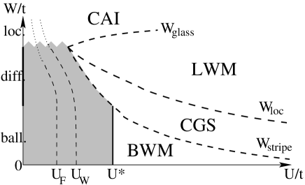
Figure 18: Different lattice regimes for $N=3$ spinless fermions in $L\times L$ disordered lattices. The shaded part of the $\left(U/t,W/t\right)$ plane gives the continuum regimes where $I$ does not depend on $U/t$. The thick dashed lines give the threshold values $W_{stripe}$ and $W_{loc}$ and $W_{glass}$ separating different lattice regimes. $U^{*}$, $U_{W}$ and $U_{F}$ are defined in section 3. The continuum and lattice CAI regimes occuring at large disorders are not separated.

We have sketched in Fig.18 the different lattice regimes characterizing $N=3$ spinless fermions in the plane $\left(U/t,W/t\right)$. The shaded part of the $\left(U/t,W/t\right)$ plane gives the continuum regimes which we will study in more details in section 9. The non shaded part gives the lattice regimes which we have studied. Let us summarize the behaviors obtained by increasing $U$ for small disorder strengths $W$.

When $W=0$, one gets between $U_{F}$ and $U_{W}$ a continuum supersolid molecule between the Fermi system and the continuum Wigner molecule before having a lattice Wigner molecule above $U^{*}$ (see section 5).

When $W/t<1$ and $L\approx 6-9$, the continuum ballistic regimes are followed by three lattice regimes taking place above $U^{*}/t$: a BWM regime for $U^{*}<U<U_{stripe}$; a CGSC regime for $U_{stripe}<U<U_{loc}$ and eventually a LWM regime above $U_{loc}$. The disorder is irrelevant below $U_{stripe}$, unless the system is at the vicinity of an avoided level crossing.

When $W/t$ is large enough to yield Anderson localization inside a small scale $L\approx 6-9$, the Fermi glass with Anderson localization (CAI regime) becomes a highly correlated solid as $U$ increases, through an intermediate regime studied in Ref. bwp1 . Three examples are given in Fig. 17 for $W/t=10,20,40$, showing that when $U$ exceeds $U_{glass}$, a localized regime where $I$ is independent of $U$ gives rise to another localized regime where $I$ becomes independent of $W$. In those three cases, $I_{l}$ changes its sign around $U_{glass}$. As pointed out in Refs. bwp1 ; bwp2 , the sign of $I_{l}$ fluctuates from sample to sample for weak $U$ while it becomes non-random at large $U$.

We study in the following section the effect of $U$ upon the continuum limit of a diffusive sample where $W=t=1$ for $L=6$ and $9$.

9 Analysis of the continuum regimes of a diffusive sample

For a ratio $W/t\approx 1$, there is a diffusive motion when $U/t=0$ and $L\approx 6$ or $9$. We study the continuum limit where $I$ does not exhibit the power law decays characteristic of lattice regimes. For values of $U/t$ smaller than the lattice threshold $U^{*}/t$, one can indeed see in Figs. 9 and 10 that $|I_{l}|$ and $|I_{t}|$ are almost independent of $U$, excepted around the value $U_{lc}$ where an avoided level crossing occurs. $U_{lc}$ depends on $W$ and $t$ and exhibits sample to sample fluctuations. This avoided crossing yields a change of the sign of $I_{l}$, a sharp drop of $|I_{l}|$ and singularities in $|I_{t}/I_{l}|$ (see Figs. 11 and 12). Since the total current $I$ is independent of $U/t$ outside level crossings in the continuum limit, one needs to study the local currents and the corresponding particle densities for detecting the different continuum regimes.

9.1 Continuum regime for a Coulomb Guided Stripe of Current

As one can see in Figs. 11 and 12, $|I_{t}/I_{l}|=1$ below $U^{*}/t$, while $I_{l}$ and $I_{t}$ are independent of $U$ instead of exhibiting the lattice decays. This shows us that the regime of current stripes is robust, and persists outside the lattice limit, in the continuum diffusive limit. This continuum CGSC regime is illustrated in Fig. 19. The left figure shows the map of local currents obtained in a disordered sample with $N=3$, $L=9$, $W=1$, $t=1$ and $U=50$. The current exhibits the Coulomb guided flow along the diagonal direction, while one can see in Fig. 10 that $I$ does not vary as a function of $U$ around $U=50$. The corresponding site occupation numbers given in Fig. 19 (right) form an extended diagonal stripe, instead of being localized upon three main sites, as in the CGSC lattice regime shown in Fig. 7 (right).

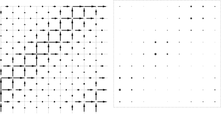
Figure 19: Coulomb guided stripe of current in the continuum limit. Disordered sample with $N=3$, $L=9$, $W=1$, $t=1$ and $U=50$. Left figure: map of currents for $\Phi=0.05\Phi_{0}$. Right figure: corresponding site occupation numbers $n_{\bf j}^{0}$.

9.2 Diamagnetic or Paramagnetic currents?

Before considering weaker values of $U$ to be closer to the quantum Fermi limit, it is useful to mention a theorem proved by Leggett leggett1 for one dimensional spinless fermions with arbitrary interaction and external potentials. This theorem allows to determine the parity of the number of particles carrying $I$ from the sign of $I$. Using a certain variational ansatz for the GS wave-function, one can show that $I$ is diamagnetic for an odd number $N$ of particles when $\Phi\approx n\Phi_{0}$ or for an even number $N$ of particles when $\Phi\approx(n+1/2)\Phi_{0}$, where $n$ is an integer. This means that the charge stiffness

$$D=\frac{(-1)^{N}L}{2}\left(E_{0}(0)-E_{0}(\pi)\right)\geq 0$$ (81)

in one dimension. To odd numbers $N$ correspond diamagnetic currents, while they are paramagnetic if $N$ is even. This result has always been verified sjwp in numerical studies of one dimensional systems with arbitrary disorders and interactions. The argument is based on the study of the nodes of the wave functions, a simple exercise in one dimension which becomes highly nontrivial and still unsolved in higher dimensions. If the transverse dimensions are small, one can argue that nodal surfaces having a two dimensional topology will cost too much kinetic energy, and that the sign of $I$ is still given by the one dimensional rule. In the square lattices which we consider, we do not use Leggett’s rule because the system is a narrow stripe, but because the Coulomb repulsion gives rise to a narrow stripe of current in the 2d lattice, reducing the two dimensional dynamics to a simpler one dimensional contribution. From the sign of $I$, one can know the parity of the effective number of particles which give rise to the observed one dimensional stripe of current.

9.3 Disordered supersolid regime

When we continue to decrease $U$, to eventually get a Fermi glass of three independent particles, we observe for $N=3$ a level crossing around $U_{lc}$ where the sign of $I$ changes. $I$ is diamagnetic above $U_{lc}$ and paramagnetic below $U_{lc}$. When $U$ is not too weak, the local currents forms a stripe of an almost one dimensional topology. This allows us to use Leggett’s rule to argue that a diamagnetic current stripe is carried by $N=3$ particles, while the paramagnetic current stripe which persists below $U_{lc}$ is due to a single delocalized pair ($N=2$ even) in the background of an almost localized third particle. Below $U_{lc}$, the correlated pair gives a dominant paramagnetic current, while the third localized particle gives rise to a negligible $2d$ current of random sign. This disordered supersolid regime seems to be associated with the $1/W$-behavior of $I$ shown in Figs. 13 and 14.

Using the same sample which displays the continuum diamagnetic stripe shown in Fig. 19 for $U=50$, one shows the map of currents and the occupation numbers $n_{\bf i}^{0}$ in Fig. 20 and Fig. 21 for $U\approx U_{lc}\approx 15$ and $U=7$ respectively. The $n_{\bf i}^{0}$ are close to those obtained in the same sample for $U=50$ (see Fig. 19). They form approximately the same stripe, though its width becomes broader. However, the map of currents are very different. As one can see in Fig. 21 for $U=7$, the current stripe shown in the left figure is perpendicular to the density stripe visible in the right figure, while there is a superposition of two perpendicular diagonal flows near the avoided level crossing ( Fig. 20). The width of the paramagnetic stripe of current increases to give a two dimensional pattern of local currents when $U\rightarrow 0$ and $W/t\approx 1$, the sign of $I$ becoming sample dependent.

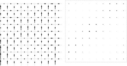
Figure 20: Behavior obtained near the avoided level crossing ($U_{lc}$) for a disordered sample with $N=3$, $L=9$, $W=1$, $t=1$ and $U=15$. Left figure: map of currents for $\Phi=0.05\Phi_{0}$. Right figure: corresponding site occupation numbers $n_{\bf j}^{0}$. The $n_{\bf j}^{0}$ are similar to those obtained in the same sample with $U=50$ (see Fig. 19) while the currents is the superposition of two perpendicular diagonal motions.

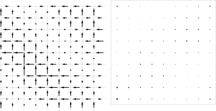
Figure 21: Behavior obtained below the paramagnetic-diamagnetic crossover for a disordered sample with $N=3$, $L=9$, $W=1$, $t=1$ and $U=7$ ($r_{s}\approx r_{s}^{F}$) . Left figure: map of currents for $\Phi=0.05\Phi_{0}$. Right figure: corresponding site occupation numbers $n_{\bf j}^{0}$. The left and right figures are now disconnected, $I$ flowing mainly perpendicularly to the axis where the $n_{\bf j}^{0}$ are maxima.

9.4 $\Phi_{0}$, $\Phi_{0}/2$ and $\Phi_{0}/3$ harmonics of $I(\Phi)$

Figure 22: $I_{l}$ as a function of $\Phi/\Phi_{0}$ for a disordered sample with $N=3$, $L=9$, $W=1$ and $t=1$ and three values of $U$. The negative (positive) currents are paramagnetic (diamagnetic) for an infinitesimal positive flux. One can see a change of sign between $U=15$ and $U=50$.

To study more precisely how melts the Wigner molecule when $U\rightarrow 0$ in a disordered sample where $L=9$, $t=W=1$, we give in Fig. 22 $I_{l}$ as a function of $\Phi$, for the values of $U$ where one expects the end of the Fermi glass ($U=5$), a disordered supersolid ($U=15$) and the continuum CGSC-regime ($U=50$) respectively. For large $U$, Leggett’s rule gives a diamagnetic molecule of $N=3$ particles, when the dynamics remains inside a 1d stripe. This rule is indeed observed for $U=50$ where $I_{l}(\Phi)$ exhibits an amplitude as large as for weaker interactions with no trace of other characteristic period than $\Phi_{0}$. In contrast, the curves obtained for $U=15$ and $U=5$ have reacher harmonic structures.

$I_{l}(\Phi)$ is an odd function of $\Phi$ ($I_{l}(\Phi)=-I(\Phi)$) of period $\Phi_{0}$ which can be expanded as:

$$I_{l}(\Phi)=\sqrt{2}\sum_{n=1}^{\infty}I_{n}\sin\left(2\pi n\frac{\Phi}{\Phi_{0}}\right)$$ (82)

where the Fourier components $I_{n}$ are

$$I_{n}=\int_{0}^{\Phi_{0}}I_{l}(\Phi)\sqrt{2}\sin\left(2\pi n\frac{\Phi}{\Phi_{0}}\right)d\Phi$$ (83)

We give in Figs. 23 and 24 the $\Phi_{0}$, $\Phi_{0}/2$ and $\Phi_{0}/3$ harmonics of $I_{l}(\Phi)$ as a function of $r_{s}$ for two disordered samples of size $L=6$ and $9$ respectively, with $W=t=1$. These harmonics, mainly $I_{1}$ and $I_{2}$, give the largest contributions. One can see that they are negative (paramagnetic) up to $r_{s}^{F}$. Around $r_{s}^{F}$, $I_{3}$ becomes positive, to reach a maximum for $r_{s}\approx 25$ where $I_{1}\approx 0$. Above $r_{s}\approx 25$, the odd harmonics $I_{1}$ and $I_{3}$ are diamagnetic, while the even harmonic $I_{2}$ remain paramagnetic. This is what Leggett’s rule gives if each $I_{n}$ was due to a $n$ body motion in one dimension. This allows us to give for each sample the characteristic values where the current topology becomes one dimensional and Leggett’s rule applies. For $U\approx 40$ in the sample shown in Fig. 24, the diamagnetic $I_{1}$ is maximum while the two others are negligible, and one has the continuum stripe (CGS-regime) shown in Fig. 19. The period $\Phi_{0}$ should be expected for a continuum disordered stripe, a $L/3,L/3$ translation of each of the $3$ particles being equivalent to have a single particle enclosing $\Phi_{0}$.

Figure 23: Harmonics $I_{n}$ characterizing the period $\Phi_{0}/n$ of the longitudinal current $I_{l}(\Phi)$ as a function of $r_{s}$ for a disordered sample with $N=3$, $L=6$, $W=1$ and $t=1$.

Figure 24: Harmonics $I_{n}$ characterizing the period $\Phi_{0}/n$ of the longitudinal current $I_{l}(\Phi)$ as a function of $r_{s}$ for a disordered sample with $N=3$, $L=9$, $W=1$ and $t=1$.

10 Summary

Considering only $N=3$ spinless fermions in a 2d square lattice with random potentials, we have obtained many different regimes by increasing the strength $U$ of the electronic correlations. Studying how $I$ depends on the system parameters, we have distinguished the continuum regimes from the lattice regimes. Increasing $U$ in a disordered sample of size $L$, we have studied the effect of electronic correlations in the ballistic, diffusive and localized regimes without interaction. Looking at the map of local currents induced by a flux $\Phi$, we have identified two regimes reminiscent of phases discussed in other fields, the stripes in the theory of strongly correlated electrons and the supersolids in the theory of quantum solids.

In the regime of the current stripe, the observed diagonal motion is clearly characteristic of the oblique shape of the Wigner molecule with $N=3$. For larger $N$, it is likely that one has a regime where the current flows along the axes of the Wigner crystal. If those axes form an angle with the shortest direction enclosing the flux, the ratio $I_{t}/I_{l}\neq 0$. When the electron crystal is pinned by disorder, this suggests that one can have an anisotropic resistivity tensor inside a certain range of density. Similar behaviors are observed in cuprate oxides with high temperature superconductivity in a certain range of chemical doping and in 2DEGs under high perpendicular magnetic fields. More directly related to our problem, the existence of stripe phases in 2DEGs is also discussed in Ref. spivak3 .

The nature of the intermediate regime between the solid and the liquid is a more delicate issue. We suggest that one could have a “supersolid”. This concept was introduced long ago to describe the quantum melting of 3d quantum solids at very low temperature when the pressure is varied. Decades of studies of Helium-3 (fermions) or Helium-4 (bosons) atoms have not allowed to reach a firm conclusion. Very recent experiments by Kim and Chan in solid Helium-4 today ; kim1 ; kim2 ; leggett2 can be interpreted as an observation of an apparent superfluid component, suggesting that a melting solid could have a supersolid fraction at certain intermediate pressures. For electrons in two dimensions, a supersolid phase is a possibility mentioned in Refs ksp ; np . One can also mention other possibilities. For instance a quantum liquid crystal bwp2 (quantum hexatic phase), in analogy with the thermal melting of an electron crystal of very large $r_{s}$. Clearly, more works are needed to understand more precisely the exact nature of the 2DEG at intermediate values of $r_{s}$. Let us conclude by summarizing three facts characterizing the intermediate values of $r_{s}$ : (i) the existence of an unexpected 2d-metallic behavior given by transport measurements, (ii) the particular maps of local persistent currents obtained in exact numerical studies using a few spinless fermions, obtained in this work or in Refs bwp1 ; bwp2 ; avishai ; sp ; ksp ; np , (iii) the results of a recent fixed node Monte Carlo study fw using $N\approx 50-200$ spinless fermions and extrapolated to the limit $N\rightarrow\infty$ which show that the nodal structure of a Slater determinant of delocalized Bloch waves gives a smaller GS energy than the trial wave-functions previously used to describe either a pure solid or a pure liquid, for intermediate values of $r_{s}$ ($30<r_{s}<80$).

Z. Á. Németh acknowledges the financial support provided through the European Community’s Human Potential Programme under contract HPRN-CT-2000-00144.

References

- (1) E. Abrahams, S.V. Kravchenko and M.P. Sarachik, Rev. Mod. Phys. 73, 251 (2001) and refs therein.
- (2) J. Yoon, C.C. Li, D. Shahar, D.C. Tsui and M. Shayegan, Phys. Rev. Lett. 82, 1744 (1999).
- (3) M.Y. Simmons, A.R. Hamilton, M. Pepper, E.H. Linfeld, P.D. Rose and D.A. Ritchie, Phys. Rev. Lett. 84, 2489 (2000).
- (4) G. Benenti, X. Waintal and J.-L. Pichard, Phys. Rev. Lett. 83, 1826 (1999).
- (5) G. Benenti, X. Waintal and J.-L. Pichard, Europhys. Lett. 51, 89 (2000).
- (6) R. Berkovits and Y. Avishai, Phys. Rev. B 57, R15076 (1998).
- (7) F. Selva and J.-L. Pichard, Europhys. Lett. 55, 518 (2001).
- (8) G. Katomeris, F. Selva and J.-L. Pichard, Eur. Phys. J. B 31 401 (2003).
- (9) Z. Á. Németh and J.-L. Pichard, Eur. Phys. J. B 33 8799 (2003).
- (10) A. F. Andreev and I. M. Lifshitz, Sov. Phys. JETP 29, 1107 (1969).
- (11) I. E. Dzyaloshinskii, P. S. Kondatenko and V. S. Levchenko, JETP 35 (1972) 823 and 1213.
- (12) B.I. Spivak, Phys. Rev. B 67, 125205 (2003).
- (13) R. Jamei, S.A. Kivelson and B.I. Spivak, Phys. Rev. Lett. 94, 056805 (2005).
- (14) B. Tanatar and D.M. Ceperley, Phys. Rev. B 39, 5005 (1989).
- (15) H. Falakshahi and X. Waintal, Phys. Rev. Lett. 94, 046801 (2005).
- (16) H. Falakshahi. Ph-D Thesis, University of Paris-Sud (Orsay) (2004).
- (17) X. Waintal, G. Benenti, and J.-L. Pichard, Europhys. Lett. 49, 466 (2000).
- (18) M. Martínez and J.-L. Pichard, Eur. Phys. J. B. 30, 93 (2002).
- (19) H. Falakshahi, Z. Á. Németh and J.-L. Pichard, Eur. Phys. J. B. 39, 93 (2004).
- (20) A. Müller-Groeling and H.A. Weidenmüller, Phys. Rev. B 49, 4752 (1994).
- (21) I.V. Krive, P. Sandström, R.I. Shekhter, S.M. Girvin and M. Jonson, Phys. Rev. B 52, 16451 (1995).
- (22) G. Burmeister and K. Maschke, Phys. Rev. B 65, 155333 (2002).
- (23) P.N. Walker, G. Montambaux, and Y. Gefen, Phys. Rev. B 60, 2541 (1999).
- (24) E. V. Tsiper and A. L. Efros, Phys. Rev. B 57, 6949 (1998).
- (25) F. Selva and D. Weinmann, Eur. Phys. J. B 18, 137 (2000).
- (26) H. F. Cheung, E. K. Riedel and Y. Gefen, Phys. Rev. Lett. 62, 587 (1989).
- (27) G. Montambaux, H. Bouchiat, D. Sigeti and R. Friesner, Phys. Rev. B 42, 7647 (1990).
- (28) J. Kroha, Physica A 167, 231 (1990).
- (29) A. J. Leggett, in Granular Nanoelectronics, edited by D. K. Ferry, Plenum, New York, 297 (1991).
- (30) P. Schmitteckert, R.A. Jalabert, D. Weinmann, and J.-L. Pichard, Phys. Rev. Lett. 81, 2308 (1998).
- (31) B.I. Spivak and S.A. Kivelson, cond-mat/0310712.
- (32) S. K. Blau, Physics Today, 23 , November 2004.
- (33) E.S. Kim and M.H.W. Chan, Nature 427, 225 (2004).
- (34) E.S. Kim and M.H.W. Chan, Science 305, 1941 (2004).
- (35) A.J. Leggett, Science 305, 1921 (2004).