Quantum Noise in the Electromechanical Shuttle

Abstract

We consider a type of Quantum Electro-Mechanical System, known as the shuttle system, first proposed by Gorelik et al. , [Phys. Rev. Lett., 80, 4526, (1998)]. We use a quantum master equation treatment and compare the semi-classical solution to a full quantum simulation to reveal the dynamics, followed by a discussion of the current noise of the system. The transition between tunnelling and shuttling regime can be measured directly in the spectrum of the noise.

I Introduction

Nanofabrication techniques, combined with single electronics, have recently enabled position measurements on an electromechanical oscillator to approach the Heisenberg limitknobel-cleland ; lahaye ; ekinci . In this paper we present a master equation treatment of a version of a quantum electromechanical system (QEMS), the charge shuttle, first proposed by Gorelik gorelik . In the original proposal a metallic grain is surrounded by elastic soft organic molecules and placed between two electrodes. This forms a Single Electron Transistor (SET) with a movable island. The coupling between the vibration of the island and the tunnelling onto the SET island dramatically alters the transport properties of the SET. The tunnelling amplitudes between the reservoirs and the island are an exponential function of the separation between island and the reservoirs. If the island is oscillating with a non negligible amplitude, this separation is a function of the displacement of the island from equilibrium and thus the tunneling current is modulated by the motion of the island. When there is a non-zero charge on the island the applied electric field accelerates the island. As the electron number on the island is a stochastic quantity, the resulting applied force is itself stochastic, but constant for a given electron occupancy of the island. Assuming the restoring force on the island can be approximated as harmonic, we have a picture of a system moving on multiple quadratic potential surfaces, with differing equilibrium displacements, connected by conditional Poisson processes corresponding to tunneling of electrons on and off the island. The shuttle thus provides a fascinating example of a quantum stochastic system in which electron transport and vibrational motion are strongly coupled.

In this paper we idealise the island to a single quantum dot with only one quasi-bound electronic state. This corresponds to an extreme Coulomb blockade regime in which the energy required for double occupancy is not bound. This minimal model captures the essential quantum stochastic dynamics of the shuttle system. The quantum dot jumps between two quadratic potential surfaces, displaced from each other, corresponding to no electron on the island and one electron on the island. As noted by previous authors, the system exhibits rich dynamics including a fixed point to limit cycle bifurcation in which the average electron occupation number on the island exhibits a periodic square wave dependence. In this paper we give a quantum master equation treatment of this quantum stochastic dynamical system, with particular attention to the shuttling and the current noise spectrum. We use the Quantum Optics Toolboxqotoolbox to compare and contrast the well known semiclassical predictions to the full quantum dynamics. In particular, we compare the picture of ensemble averaged dynamics of various moments with a ‘quantum trajectory’molmer simulation of moments. A quantum trajectory is a concept taken from quantum optics to describe the conditional dynamics of the system conditioned on a particular history of stochastic events. Such conditional dynamics provide insight into the effect of quantum noise on the the semiclassical prediction of regular electron shuttling on the limit cycle.

Various versions of a charge shuttle system have been experimentally investigated. A review of the theoretical and experimental achievements in shuttle transport can also be found in the work of Shekhter et al.shekhter . When a voltage bias is applied between the electrodes, a current quantisation resulting from electron interactions with the vibrational levels for different voltage bias was found. By using C₆₀ embedded between two gold electrodes, Park et al. park have demonstrated that indeed there is current quantisation for various bias voltage which results in a stair-like feature within the current-voltage curve. Although because of its high frequency (around Terra Hertz) and low amplitude oscillation, the molecule hardly shuttles between the electrodes in this setup, this experiment has provided key evidence of the involvement of vibrational levels in changing the properties of the current. This quantized conductance also was observed in several other experiments zhitenev ; erbe . Zhitenev et al. zhitenev utilize metal single electron transistor attached on the tip of quartz rods as scanning probe while the experiment by Erbe et al. erbe , combines a nanomechanical resonator with an electron island to produce a QEMS system. The experimental setup used by Erbe is similar to the one proposed by Gorelik gorelik . Huang et al. also reported the operation of a GHz mechanical oscillatorhuang .

Several attempts to explain the behaviour of the system have been offered both from classical and quantum point of view. The current quantisation and its low frequency noise was investigated via a classical approach by Isacsson isacsson_noise . The current-voltage relation in the shuttle system exists within two regimes. The first regime is when the electron tunnels straight into the dot from the source and off to the drain, without much involvement of the island movement. This is called the tunnel regime. The C₆₀ system lies within this tunnel regime. The other regime is when the island oscillates to accommodate the current flow, which we call the shuttle regime. However, measurement of average current alone cannot provide enough information to distinguish whether the system is in the shuttle regime or tunnel regime. It was shown that a calculation of the noise is needed in addition. Therefore the noise signature was first obtained by finding the Fano factor at zero frequency novotny_shot . Recently Flindt et al.flindt have calculated the current noise spectrum using a method different form that used in this paper. We compare the two methods in section VI.

Another interesting property of the system is the existence of a dynamical instability with limit-cycle behavior which was found in a similar setup using a single metallic grain placed on a cantilever between two electrodes isacsson . This forms a three-terminal contact shuttle system. Classical analysis of the system points to the fact that this instability in the system leads to deterministic chaos. The semiclassical dynamics of the simpler case of the isolated island, the subject of this paper, was thoroughly investigated by Donarini et al. donarini .

One of the early attempt to investigate the system within the quantum limit is given by Aji et al. aji where electronic-vibrational coupling is investigated both in elastic and inelastic electron transport by looking at the current-voltage relationship and conductance. Other properties of the transport within the shuttle system such as negative differential conductance have also been found mccarthy although the derivation only considers terms linear in the position of the island. Various conditions, such as when the electron tunnelling length is much greater than the amplitude of the zero point oscillations of the central island, have been investigated by Fedoretsfedorets_shuttle . Using phase space methods in terms of Wigner function Novotny et al. novotny ; jauho identify crossover from tunnelling to shuttling regime.

Another variation of the shuttle is offered by Armour and MacKinnon armourandmackinon . In this model the steady state current across a chain of three quantum dots system (one dot connected to each leads and one dot as vibrating island) was analysed by looking at the eigenspectrum. Numerical simulation here considers 25 phonon levels, within the large bias limit.

In a recent thesis of Donarini donarini , the single dot quantum shuttle and the three dot shuttle system was investigated using Generalized Master Equation approach using Wigner distribution functions. The current and Fano factor at zero frequency is also investigated.

II The Model

The system consists of a quantum dot ’island’ moving between two electrodes, the source and the drain. This is analogous to a quantum dot SET in which the island of the SET is allowed to oscillate and thus modulate the tunnel conductance between itself and the reservoirs. However unlike a SET we do not include a separate charging gate for the island. When a voltage bias is applied between the two electrodes, the electron from the source can tunnel onto the island and as the island moves closer to the drain the electron can tunnel off, thus producing a current. Here we assume that only one electronic level is available within the island, a condition of strong coulomb blockade.

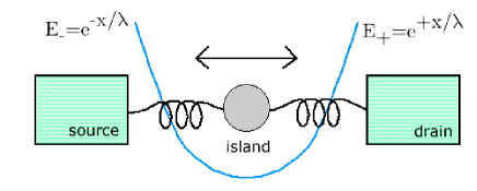
Figure 1: Schematic representation of shuttling between a source and a drain through a quantum dot.

The electronic single quasi-bound state on the dot is described by Fermi annihilation and creation operators $c,c^{\dagger}$, which satisfy the anti commutation relation $cc^{\dagger}+c^{\dagger}c=1$. While the vibrational degree of freedom is described by a displacement operator $\hat{x}$ which can be written in terms of annihilation and creation operators $a$ and $a^{\dagger}$, with the commutation relation $aa^{\dagger}-a^{\dagger}a=1$.

$$\hat{x}=\sqrt{\frac{{\mathchoice{{\raisebox{-1.42082pt}{$\displaystyle\mathchar 22\relax$}\mkern-7.2muh}}{{\raisebox{-1.42082pt}{$\displaystyle\mathchar 22\relax$}\mkern-7.2muh}}{{\raisebox{-0.25832pt}{$\scriptstyle\mathchar 22\relax$}\mkern-7.2muh}}{{\raisebox{-0.08612pt}{$\scriptscriptstyle\mathchar 22\relax$}\mkern-7.2muh}}}}{2m\nu}}(a+a^{\dagger}).$$ (1)

The Hamiltonian of the system is given by:

$$H={\mathchoice{{\raisebox{-1.42082pt}{$\displaystyle\mathchar 22\relax$}\mkern-7.2muh}}{{\raisebox{-1.42082pt}{$\displaystyle\mathchar 22\relax$}\mkern-7.2muh}}{{\raisebox{-0.25832pt}{$\scriptstyle\mathchar 22\relax$}\mkern-7.2muh}}{{\raisebox{-0.08612pt}{$\scriptscriptstyle\mathchar 22\relax$}\mkern-7.2muh}}}\omega_{I}c^{\dagger}c+U_{c}\hat{n}^{2}$$ (7)

$$+\hskip 2.84544pt{\mathchoice{{\raisebox{-1.42082pt}{$\displaystyle\mathchar 22\relax$}\mkern-7.2muh}}{{\raisebox{-1.42082pt}{$\displaystyle\mathchar 22\relax$}\mkern-7.2muh}}{{\raisebox{-0.25832pt}{$\scriptstyle\mathchar 22\relax$}\mkern-7.2muh}}{{\raisebox{-0.08612pt}{$\scriptscriptstyle\mathchar 22\relax$}\mkern-7.2muh}}}\nu a^{\dagger}a$$

$$+\hskip 2.84544pt{\mathchoice{{\raisebox{-1.42082pt}{$\displaystyle\mathchar 22\relax$}\mkern-7.2muh}}{{\raisebox{-1.42082pt}{$\displaystyle\mathchar 22\relax$}\mkern-7.2muh}}{{\raisebox{-0.25832pt}{$\scriptstyle\mathchar 22\relax$}\mkern-7.2muh}}{{\raisebox{-0.08612pt}{$\scriptscriptstyle\mathchar 22\relax$}\mkern-7.2muh}}}{\omega_{s}ka_{k}^{\dagger}a_{k}+{\mathchoice{{\raisebox{-1.42082pt}{$\displaystyle\mathchar 22\relax$}\mkern-7.2muh}}{{\raisebox{-1.42082pt}{$\displaystyle\mathchar 22\relax$}\mkern-7.2muh}}{{\raisebox{-0.25832pt}{$\scriptstyle\mathchar 22\relax$}\mkern-7.2muh}}{{\raisebox{-0.08612pt}{$\scriptscriptstyle\mathchar 22\relax$}\mkern-7.2muh}}}\omega_{d}kb_{k}^{\dagger}b_{k}}$$

$$-\hskip 2.84544pteE\ \hat{x}\ c^{\dagger}c$$

$$+\hskip 2.84544pt\sum_{k}(T_{sk}E_{-}(\hat{x})a_{k}c^{\dagger}+{\rm h.c})+\sum_{k}(T_{dk}E_{+}(\hat{x})b_{k}c^{\dagger}+{\rm h.c})$$

$$+\hskip 2.84544pt\sum_{p}g(a^{\dagger}d_{p}+ad_{p}^{\dagger})+\sum_{p}{\mathchoice{{\raisebox{-1.42082pt}{$\displaystyle\mathchar 22\relax$}\mkern-7.2muh}}{{\raisebox{-1.42082pt}{$\displaystyle\mathchar 22\relax$}\mkern-7.2muh}}{{\raisebox{-0.25832pt}{$\scriptstyle\mathchar 22\relax$}\mkern-7.2muh}}{{\raisebox{-0.08612pt}{$\scriptscriptstyle\mathchar 22\relax$}\mkern-7.2muh}}}\omega_{p}d_{p}^{\dagger}d_{p},$$

where $E$ is the electric field seen by an electron on the dot.

The first term of the Hamiltonian describes the energy of a single-electron quasi-bound state of the island. For the purpose of our simulation, we will scale other energies in terms of this island energy and thus conveniently set ${\mathchoice{{\raisebox{-1.42082pt}{$\displaystyle\mathchar 22\relax$}\mkern-7.2muh}}{{\raisebox{-1.42082pt}{$\displaystyle\mathchar 22\relax$}\mkern-7.2muh}}{{\raisebox{-0.25832pt}{$\scriptstyle\mathchar 22\relax$}\mkern-7.2muh}}{{\raisebox{-0.08612pt}{$\scriptscriptstyle\mathchar 22\relax$}\mkern-7.2muh}}}\omega_{I}=1$. The Coulomb charge energy, $U_{c}$ is the energy that is required to add an electron when there is already one electron occupying the island ($\hat{n}=c^{\dagger}c$). This energy is assumed to be large enough so that no more than one electron occupies the island at any time. This is the Coulomb blockade regime. In this regime it is better to regard the island as a single quantum dot rather than a metal island and we will refer to it as such in the remainder of this paper. The free Hamiltonian for the oscillator is described in term (7) where $\nu$ is the frequency of the mechanical oscillation of the quantum dot. The electrostatic energy of electrons in the source ($s$) and drain ($d$) reservoirs is written as term (7). With $a_{k},a_{k}^{\dagger}$ and $b_{k},b_{k}^{\dagger}$ the annihilation and creation operator for the electron in the source and drain respectively. Term (7) describes the electrostatic coupling between the oscillator and charge while term (7) represents the source-island tunnel coupling and the drain-island tunnel coupling. In the shuttle system, the island of the SET is designed to move between the source and the drain terminal with an amplitude or fluctuation comparable to the distance of the island to the lead. Thus we introduce the term

$$E_{\pm}(\hat{x}) = e^{\pm\hat{x}/\lambda}$$ (8)

$$= e^{\pm\eta(a+a^{\dagger})}$$ (9)

with

$$\eta=\left(\frac{{\mathchoice{{\raisebox{-1.42082pt}{$\displaystyle\mathchar 22\relax$}\mkern-7.2muh}}{{\raisebox{-1.42082pt}{$\displaystyle\mathchar 22\relax$}\mkern-7.2muh}}{{\raisebox{-0.25832pt}{$\scriptstyle\mathchar 22\relax$}\mkern-7.2muh}}{{\raisebox{-0.08612pt}{$\scriptscriptstyle\mathchar 22\relax$}\mkern-7.2muh}}}}{2m\nu}\right)^{1/2}\frac{1}{\lambda}$$ (10)

to account for the change in the tunnelling rate to the left and the right lead as the position of the shuttle varies.

The last term, (7), describes the coupling between the oscillator and the thermo-mechanical bath responsible for damping and thermal noise in the mechanical system in the rotating wave approximationgardiner-zoller . We include it in order to bound the motion under certain bias conditions.

We now obtain a closed evolution for the system of quantum dot plus oscillator by tracing out over the degrees of freedom in the leads. A Markov master equation for the island-oscillator system can then be derived in the Born and Markov approximation using standard techniqueswahyu . If we assume the vibrational frequency of the oscillator is slow compared to bath relaxation time scales, we arrive at:

$$\dot{\rho} = -i\nu[a^{\dagger}a,\rho]$$ (11)

$$+ i\chi[(a+a^{\dagger})c^{\dagger}c,\rho]$$

$$+ \gamma_{L}\bigl{(}f({\mathchoice{{\raisebox{-1.42082pt}{$\displaystyle\mathchar 22\relax$}\mkern-7.2muh}}{{\raisebox{-1.42082pt}{$\displaystyle\mathchar 22\relax$}\mkern-7.2muh}}{{\raisebox{-0.25832pt}{$\scriptstyle\mathchar 22\relax$}\mkern-7.2muh}}{{\raisebox{-0.08612pt}{$\scriptscriptstyle\mathchar 22\relax$}\mkern-7.2muh}}}\omega_{I}-\mu_{L})\mathcal{D}[c^{\dagger}E_{-}(\hat{x})]\rho+(1-f({\mathchoice{{\raisebox{-1.42082pt}{$\displaystyle\mathchar 22\relax$}\mkern-7.2muh}}{{\raisebox{-1.42082pt}{$\displaystyle\mathchar 22\relax$}\mkern-7.2muh}}{{\raisebox{-0.25832pt}{$\scriptstyle\mathchar 22\relax$}\mkern-7.2muh}}{{\raisebox{-0.08612pt}{$\scriptscriptstyle\mathchar 22\relax$}\mkern-7.2muh}}}\omega_{I}-\mu_{L}))\mathcal{D}[cE_{-}(\hat{x})]\rho\bigr{)}$$

$$+ \gamma_{R}\bigl{(}f({\mathchoice{{\raisebox{-1.42082pt}{$\displaystyle\mathchar 22\relax$}\mkern-7.2muh}}{{\raisebox{-1.42082pt}{$\displaystyle\mathchar 22\relax$}\mkern-7.2muh}}{{\raisebox{-0.25832pt}{$\scriptstyle\mathchar 22\relax$}\mkern-7.2muh}}{{\raisebox{-0.08612pt}{$\scriptscriptstyle\mathchar 22\relax$}\mkern-7.2muh}}}\omega_{I}-\mu_{R})\mathcal{D}[c^{\dagger}E_{+}(\hat{x})]\rho+(1-f({\mathchoice{{\raisebox{-1.42082pt}{$\displaystyle\mathchar 22\relax$}\mkern-7.2muh}}{{\raisebox{-1.42082pt}{$\displaystyle\mathchar 22\relax$}\mkern-7.2muh}}{{\raisebox{-0.25832pt}{$\scriptstyle\mathchar 22\relax$}\mkern-7.2muh}}{{\raisebox{-0.08612pt}{$\scriptscriptstyle\mathchar 22\relax$}\mkern-7.2muh}}}\omega_{I}-\mu_{R}))\mathcal{D}[cE_{+}(\hat{x})]\rho\bigr{)}$$

$$+ \kappa(\bar{n}_{p}+1)\mathcal{D}[a]\rho+\kappa\bar{n}_{p}\mathcal{D}[a^{\dagger}]\rho,$$

with $\chi=eE\eta\lambda$ and $\bar{n}_{p}$ is the mean phonon number for the vibrational damping reservoir. We also have defined

$${\cal D}[A]\rho=A\rho A^{\dagger}-\frac{1}{2}(A^{\dagger}A\rho+\rho A^{\dagger}A),$$ (12)

where $f$ is the Fermi function $f(\epsilon)=1/(e^{\epsilon/T_{\rm el}}+1)$. This Fermi function has an implicit dependence on the temperature, $T_{\rm el}$, of the electronic system and the bias conditions between the source and the drain. The terms $\gamma_{L},\gamma_{R}$ describe the rates of electron tunnelling form the source to the dot and dot to drain respectively. We have implicitly ignored co-tunnelling and higher order scattering events, so this equation applies under weak bias and weak tunnelling conditions. The final two terms proportional to $\kappa$ describe the damping of the oscillator, where $\bar{n}_{p}=1/(e^{{\mathchoice{{\raisebox{-0.99458pt}{$\displaystyle\mathchar 22\relax$}\mkern-7.2muh}}{{\raisebox{-0.99458pt}{$\displaystyle\mathchar 22\relax$}\mkern-7.2muh}}{{\raisebox{-0.18082pt}{$\scriptstyle\mathchar 22\relax$}\mkern-7.2muh}}{{\raisebox{-0.06029pt}{$\scriptscriptstyle\mathchar 22\relax$}\mkern-7.2muh}}}\nu/k_{B}T}-1)$ and $T$ are respectively the mean excitation and the effective temperature of a thermal bath responsible for this damping process. Thermal mechanical fluctuations in the metal contacts of the source and drain cause fluctuations in position of the center of the trapping potential confining the island, that is to say small, fluctuating linear forces act on the island. For a harmonic trap, this appears to the oscillator as a thermal bath. However such a mechanism is expected to be very weak. This fact, together with the very large frequency of the oscillator, justifies our use of the quantum optical master equation (as opposed to the Brownian motion master equation) to describe this source of dissipation gardiner-zoller .

In order to discuss the phenomenology of this system we first consider a special case. Under appropriate bias conditions and very low temperature, the quasi bound state on the island is well below the Fermi level in the source and well above the Fermi level in the drain. The master equation then takes the “ zero temperature” form

$$\dot{\rho} = -i\nu[a^{\dagger}a,\rho]+i\chi[(a+a^{\dagger})c^{\dagger}c,\rho]$$ (13)

$$+ \gamma_{L}\mathcal{D}[c^{\dagger}E_{-}(\hat{x})]\rho+\gamma_{R}\mathcal{D}[cE_{+}(\hat{x})]\rho\bigr{)}$$

$$+ \kappa(\bar{n}_{p}+1)\mathcal{D}[a]\rho+\kappa\bar{n}_{p}\mathcal{D}[a^{\dagger}]\rho.$$

The terms proportional to $\gamma_{L}$ and $\gamma_{R}$ describe two conditional Poisson processes, $dN_{L}(t),dN_{R}(t)$, in which an electron tunnels on to or off the island. The average rate of these processes is given by goan_continuous ; goan_dynamics ; goan_montecarlo

$$\mathcal{E}(dN_{L}(t)) = \gamma_{L}{\rm Tr}[E_{-}(\hat{x})c^{\dagger}\rho cE_{-}(\hat{x})]dt,$$

$$\mathcal{E}(dN_{R}(t)) = \gamma_{R}{\rm Tr}[E_{+}(\hat{x})c\rho c^{\dagger}E_{+}(\hat{x})]dt.$$

where $\mathcal{E}$ refers to a classical stochastic average. Using the cyclic property of trace and the definition in Eq.(9) we see that

$$\mathcal{E}(dN_{L}(t)) = \gamma_{L}\langle e^{-2\hat{x}/\lambda}cc^{\dagger}\rangle dt,$$ (14)

$$\mathcal{E}(dN_{R}(t)) = \gamma_{R}\langle e^{2\hat{x}/\lambda}c^{\dagger}c\rangle dt.$$ (15)

It is now possible to see that the current through the dot will depend on the position of the oscillator. Under appropriate operating conditions (discussed below) we can use this dependance to configure the device as a position sensor or weak force detector. For a symmetric case where the tunnel-junction capacitances are almost the same, $C_{L}\approx C_{R}$ (neglecting the position dependence of the capacitances), the Ramo-Shockley theorem indicates that the average current in the circuit can be given by

$$I(t)=\mathcal{E}(i(t))=\frac{e}{2}\left[\mathcal{E}\left(\frac{dN_{L}(t)}{dt}\right)+\mathcal{E}\left(\frac{dN_{R}(t)}{dt}\right)\right].$$ (16)

If $\eta\ll 1$ and $\gamma_{L}=\gamma_{R}=\gamma$ we may write this as

$$I(t) \approx e\gamma/2+\frac{e\gamma}{\lambda}\langle\hat{x}(c^{\dagger}c-cc^{\dagger})\rangle+\frac{e\gamma}{\lambda^{2}}\langle\hat{x}^{2}\rangle$$ (17)

$$= e\gamma/2+\frac{e\gamma}{\lambda}(\langle\hat{x}\rangle_{1}-\langle\hat{x}\rangle_{0})+\frac{e\gamma}{\lambda^{2}}\langle\hat{x}^{2}\rangle,$$ (18)

where

$$\langle\hat{x}\rangle_{k}={\rm Tr}_{osc}[\hat{x}\langle k|\rho|k\rangle]$$ (19)

with $k=0,1$ the occupation number states for the dot, and $osc$ indicates a trace with respect to the oscillator Hilbert space alone. It is apparent that $\langle\hat{x}\rangle_{k}$ refers to the average position of the oscillator conditioned on a particular occupation of the dot. Clearly the average current through the system depends on the position of the oscillating dot. However the dependence on the first moment of position may be very weak. If the tunnel rates through the dot are much larger than all other time scales we expect that the occupation of the dot will reach an equilibrium value of $\frac{1}{2}$ quickly. In this case the term linear in position will be very small, leaving only a quadratic dependence. However if it can be arranged that $\gamma_{L}\neq\gamma_{R}$, there will be a direct dependance of the current on the oscillator position. To clarify this situation we first look at a semiclassical description of the dynamics.

III Semiclassical dynamics

The master equation Eq.(11)enables us to calculate the coupled dynamics of the vibrational and electronic degrees of freedom. The equations of motion for the occupation number on the dot and the average phonon number are

$$\frac{d\langle c^{\dagger}c\rangle}{dt} = \gamma_{L}[f_{L}\langle cc^{\dagger}e^{-2\hat{x}/\lambda}\rangle-(1-f_{L})\langle c^{\dagger}ce^{-2\hat{x}/\lambda}\rangle]$$ (20)

$$\mbox{}+\gamma_{R}[f_{R}(\langle cc^{\dagger}e^{2\hat{x}/\lambda}\rangle-(1-f_{R})\langle c^{\dagger}ce^{2\hat{x}/\lambda}\rangle],$$

$$\frac{d\langle a^{\dagger}a\rangle}{dt} = \gamma_{L}\eta^{2}[f_{L}\langle cc^{\dagger}e^{-2\hat{x}/\lambda}\rangle+(1-f_{L})\langle c^{\dagger}ce^{-2\hat{x}/\lambda}\rangle]$$ (21)

$$\mbox{}+\gamma_{R}\eta^{2}[f_{R}\langle cc^{\dagger}e^{2\hat{x}/\lambda}\rangle+(1-f_{R})\langle c^{\dagger}ce^{-2\hat{x}/\lambda}\rangle]$$

$$\mbox{}-i\chi\langle(a-a^{\dagger})c^{\dagger}c\rangle+\kappa\bar{n}-\kappa\langle a^{\dagger}a\rangle,$$

where the Fermi factors are defined by $f_{\alpha}=f(\omega_{I}-\mu_{\alpha})$ with $\alpha=L,R$ and $\mu_{\alpha}$ is the chemical potential in the source ($\alpha=L$) and drain ($\alpha=R$) and ${\mathchoice{{\raisebox{-1.42082pt}{$\displaystyle\mathchar 22\relax$}\mkern-7.2muh}}{{\raisebox{-1.42082pt}{$\displaystyle\mathchar 22\relax$}\mkern-7.2muh}}{{\raisebox{-0.25832pt}{$\scriptstyle\mathchar 22\relax$}\mkern-7.2muh}}{{\raisebox{-0.08612pt}{$\scriptscriptstyle\mathchar 22\relax$}\mkern-7.2muh}}}\omega_{I}$ is the energy of the quasi bound state on the dot. The equation of motion for the average amplitude is relatively simple:

$$\frac{d\langle a\rangle}{dt} = -i\nu\langle a\rangle-\mbox{$\frac{1}{2}$}\kappa\langle a\rangle+i\chi\langle c^{\dagger}c\rangle$$ (22)

which is the equation of motion for a damped oscillator with time dependent driving. Unfortunately these first order number moments are coupled into higher order moments generating a hierarchy of coupled equations. A semiclassical approximation to the dynamics may be defined by factorising moments for electronic and vibrational degrees of freedom. This discards quantum correlations and thus is certainly not the appropriate way to describe a quantum limited measurement. However it does enable us to see the essential features of the dynamical character of this problem. We will return to the full quantum problem in the next section.

We begin the semi-classical approach by factoring moments of oscillator and electronic coordinates, for example of $\langle cc^{\dagger}E_{-}^{2}\rangle$ into $\langle cc^{\dagger}\rangle$ $\langle E_{-}^{2}\rangle$, to obtain

$$\frac{d\langle c^{\dagger}c\rangle}{dt} = \gamma_{L}(\langle E_{-}^{2}\rangle f_{L}-\langle c^{\dagger}c\rangle\langle E_{-}^{2}\rangle)$$ (23)

$$+\gamma_{R}(\langle E_{+}^{2}\rangle f_{R}-\langle c^{\dagger}c\rangle\langle E_{+}^{2}\rangle).$$

Using the definitions,

$$\hat{x}=\eta\lambda(a+a^{\dagger})\ \ \ \ \ \ \ \ \hat{p}=-i\frac{{\mathchoice{{\raisebox{-1.42082pt}{$\displaystyle\mathchar 22\relax$}\mkern-7.2muh}}{{\raisebox{-1.42082pt}{$\displaystyle\mathchar 22\relax$}\mkern-7.2muh}}{{\raisebox{-0.25832pt}{$\scriptstyle\mathchar 22\relax$}\mkern-7.2muh}}{{\raisebox{-0.08612pt}{$\scriptscriptstyle\mathchar 22\relax$}\mkern-7.2muh}}}}{2\eta\lambda}(a-a^{\dagger})$$

we can write the semiclassical equations in terms of position $x=\langle\hat{x}\rangle$, momentum $p=\langle\hat{p}\rangle$ and electron number $n=\langle c^{\dagger}c\rangle$,

$$\frac{dn}{dt} = \gamma_{L}(e^{-2x/\lambda}f_{L}-ne^{-2x/\lambda})+\gamma_{R}(e^{2x/\lambda}f_{R}-ne^{2x/\lambda})$$ (24)

$$\frac{dx}{dt} = \frac{p}{m}-\frac{\kappa}{2}x$$ (25)

$$\frac{dp}{dt} = -m\nu^{2}x-\frac{\kappa}{2}p+\chi\sqrt{2m\nu{\mathchoice{{\raisebox{-1.42082pt}{$\displaystyle\mathchar 22\relax$}\mkern-7.2muh}}{{\raisebox{-1.42082pt}{$\displaystyle\mathchar 22\relax$}\mkern-7.2muh}}{{\raisebox{-0.25832pt}{$\scriptstyle\mathchar 22\relax$}\mkern-7.2muh}}{{\raisebox{-0.08612pt}{$\scriptscriptstyle\mathchar 22\relax$}\mkern-7.2muh}}}}\ n$$ (26)

where we have made the further factorisation $\langle E_{\pm}^{2}(\hat{x})\rangle=e^{\pm 2x/\lambda}$. These results agrees with the previous classical equations obtained by Isacsson isacsson , in the case of zero gate voltage on the island. We will carefully consider the regime of validity of these semiclassical equations in section V. For now we note that factorising vibrational and electronic degrees of freedom ignores any entanglement between these systems, while factorising the exponential assumes the oscillator is very well localised in position.

In the zero temperature limit and appropriate bias we have that $f_{L}=1,\ f_{R}=0$. The semiclassical equations of motion then take the form

$$\frac{dn}{dt} = \gamma_{L}(1-n)e^{-4\eta X}-\gamma_{R}ne^{4\eta X}$$ (27)

$$\frac{d\alpha}{dt} = -i\nu\alpha-\frac{\kappa}{2}\alpha+i\chi n$$ (28)

with

$$\alpha=\langle a\rangle=\langle\hat{x}\rangle/(2\lambda\eta)+i\langle\hat{p}\rangle\lambda\eta/{\mathchoice{{\raisebox{-1.42082pt}{$\displaystyle\mathchar 22\relax$}\mkern-7.2muh}}{{\raisebox{-1.42082pt}{$\displaystyle\mathchar 22\relax$}\mkern-7.2muh}}{{\raisebox{-0.25832pt}{$\scriptstyle\mathchar 22\relax$}\mkern-7.2muh}}{{\raisebox{-0.08612pt}{$\scriptscriptstyle\mathchar 22\relax$}\mkern-7.2muh}}}\equiv X+iY\ \ .$$

The system of equations, Eq.(27, 28) has a fixed point, which undergoes a hopf bifurcation.

To see this we begin by scaling the parameters by $\nu$ and $\eta$; $\frac{\gamma}{\nu}\rightarrow\gamma$, $\frac{\kappa}{\nu}\rightarrow\kappa$ and $\frac{\eta\chi}{\nu}\rightarrow\chi$ and $\nu\rightarrow 1$ by scaling time $\tau=\nu t$ and redefining $X$ and $Y$ by letting $\alpha=\eta(X+iY)$. Then

$$\frac{dn}{d\tau}=\gamma_{L}(1-n)e^{-4X}-\gamma_{R}ne^{4X}$$ (29)

$$\frac{d\alpha}{d\tau}=-i\alpha-\frac{\kappa}{2}\alpha+i\chi n.$$ (30)

The fixed point is given implicitly by

$$n_{*} = \frac{\gamma_{L}e^{-4X_{*}}}{\gamma_{L}e^{-4X_{*}}+\gamma_{R}e^{4X_{*}}}=\frac{1}{1+\frac{\gamma_{R}}{\gamma_{L}}e^{8X_{*}}},$$ (31)

$$X_{*} = \frac{\chi}{1+(\frac{\kappa}{2})^{2}}n_{*}$$ (32)

$$Y_{*} = \frac{\chi\frac{\kappa}{2}}{1+(\frac{\kappa}{2})^{2}}n_{*}$$ (33)

from which we can see that it must satisfy,

$$\chi=X_{*}(1+(\frac{\kappa}{2})^{2})(1+\frac{\gamma_{R}}{\gamma_{L}}e^{8X_{*}}).$$ (34)

At the hopf bifurcation the fixed point looses stability and a limitcycle is created. To see this, first obtain the linearized matrix about the stationary point.

$$DF=\left(\begin{array}[]{cccrrr}-A_{*}&-\frac{8\gamma_{L}\gamma_{R}}{A_{*}}&0\\ 0&-\frac{\kappa}{2}&1\\ \chi&-1&-\frac{\kappa}{2}\end{array}\right)$$

where

$$A_{*}=\gamma_{L}e^{-4X_{*}}+\gamma_{R}e^{4X_{*}}.$$

The stability of the fixed point is determined by the eigenvalues of this matrix. If one or more of the eigenvalues have positive real part the fixed point is unstable. For complex eigenvalues the transition between stable and unstable occurs when the eigenvalues are pure imaginary. Here this is when

$$\chi=\chi_{h}=\frac{A_{*}\kappa(A_{*}(A_{*}+\kappa)+1+(\frac{\kappa}{2})^{2})}{8\gamma_{L}\gamma_{R}}.$$

At $\chi=\chi_{h}$ the eigenvalues are $-(A_{*}+\kappa),\pm i\mu$ where $\mu=\sqrt{A_{*}\kappa+1+(\frac{\kappa}{2})^{2}}$ and the fixed point has a one dimensional stable manifold and a two dimensional center manifold. For $\chi<\chi_{h}$ the fixed point is stable and for $\chi>\chi_{h}$ it is unstable. This suggests a hopf bifurcation, however it is necessary to work out the stability coefficient to determine if it is subcritical, creating an unstable limitcycle or supercritical, creating a stable limitcycle. This involves some algebra. First transform the system in the vicinity of the fixed point to normal form via the matrix of eigenvectors $P$.

$$P=\left(\begin{array}[]{cccrrr}8\gamma_{L}\gamma_{R}&0&8\gamma_{L}\gamma_{R}\\ A_{*}\kappa&-A_{*}\mu&-A_{*}^{2}\\ -A_{*}\kappa(A_{*}+\frac{\kappa}{2})&-A_{*}(A_{*}+\frac{\kappa}{2})&-A_{*}(\frac{A_{*}\kappa}{2}+1+(\frac{\kappa}{2})^{2})\end{array}\right)$$

Then in normal form coordinates $\bf{u}$ $=P^{-1}(n-n_{*},\,X-X_{*},\,Y-Y_{*})^{T}$ the system becomes

$$\frac{d\bf{u}}{d\tau}=\left(\begin{array}[]{cccrrr}-(A_{*}+\kappa)&0&0\\ 0&0&-i\mu\\ 0&i\mu&0\end{array}\right)\mbox{\bf{u}}+\mbox{\bf{g}}Nl(\mbox{\bf{u}})+8\gamma_{L}\gamma_{R}\mbox{\bf{f}}(\chi-\chi_{h})(u_{1}+u_{3}),$$ (38)

where $\bf{g}$ and $\bf{f}$ are column vectors, whose entries are $g_{i}=P_{i1}^{-1},\,f_{i}=P_{i3}^{-1}.$ $Nl(\bf{u})$ is a scalar nonlinear function of $u_{i}$ obtained by perturbation. To cubic order in $u_{i}$

$$Nl({\bf u})=-4n^{\prime}X^{\prime}\sqrt{A_{*}^{2}-4\gamma_{L}\gamma_{R}}-8n^{\prime}{X^{\prime}}^{2}A_{*}-\frac{64\gamma_{L}\gamma_{R}{X^{\prime}}^{3}}{3A_{*}}$$

where

$$(n^{\prime},X^{\prime},Y^{\prime})^{T}=P\bf{u}^{T}.$$

Now the limitcycle bifurcates into the center manifold which is tangent to the $u_{1}=0$ plane. So if $u_{1}=h(u_{2},\,u_{3})$ is the equation of the center manifold through $(0,\,0,\,0)$ at $\chi=\chi_{h}$, then $h(0,\,0)=0$ and $\frac{\partial h}{\partial u_{i}}(0,\,0)=0$. This means that a Taylor series approximation to the center manifold will have no constant or linear term and so the first nonzero terms are of quadratic order in $u_{i}$ and

$$h(u_{2},\,u_{3})=a_{20}u_{2}^{2}+a_{11}u_{2}u_{3}+a_{02}u_{3}^{2}+\mbox{higher order terms},$$

for some $a_{20},\,a_{11}$ and $a_{02}.$ Now differentiating $u_{1}=h(u_{2},\,u_{3})$ gives;

$$\frac{du_{1}}{d\tau}=\frac{\partial h}{\partial u_{2}}\frac{du_{2}}{d\tau}+\frac{\partial h}{\partial u_{3}}\frac{du_{3}}{d\tau}.$$

On the center manifold $\frac{du_{i}}{d\tau}(h(u_{2},\,u_{3}),\,u_{2},\,u_{3})$ are functions of $u_{2}$ and $u_{3}$ only, so this equation can be used to calculate the coefficients $a_{i,j}$ in the Taylor series approximation to $h(u_{2},\,u_{3})$ recursively, by equating coefficients of like powers of $u_{2}$ and $u_{3}$. Once $h(u_{2},\,u_{3})$ is found this can be fed back into the equations of motion for $u_{2}$ and $u_{3}$ to obtain the approximate equations of motion on the center manifold. Finally the stability coefficient for a two dimensional system in normal form glendinning is $\displaystyle{a=\frac{1}{16}(f_{xxx}+g_{xxy}+f_{xyy}+g_{yyy})+\frac{1}{16\omega}(f_{xy}(f_{xx}+f_{yy})-g_{xy}(g_{xx}+g_{yy})-f_{xx}g_{xx}+f_{yy}g_{yy})}$ evaluated at $(0,\,0),$ where here $\omega=\mu=\sqrt{A_{*}\kappa+1+(\frac{\kappa}{2})^{2}}$. The subscripts indicate partial derivatives of function $f$ or $g$ with respect to the variables $x$ and $y$. For instance $f_{xx},f_{xxx}$ is is a short hand for 2nd and 3rd derivative of function $f$ with respect to $x$. Here the stability coefficient must be calculated numerically because the position of fixed point is only known implicitly via Eq. (34).

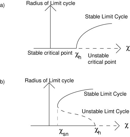
Figure 2: Illustration of two possible type of Hopf bifurcation in the shuttle system with varying coupling $\chi$, a) supercritical and b) subcritical and saddle node bifurcation of the limit cycles.

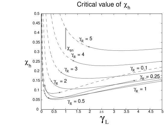
Figure 3: Plot of $\chi_{h}$ for various fixed values of $\gamma_{R}$ as a function of $\gamma_{L}$. The line is solid where the hopf bifurcation is supercritical and dashed where it is a subcritical hopf bifurcation.

Figure 3 plots $\chi_{h}$ for various fixed values of $\gamma_{R}$ as a function of $\gamma_{L}$. The line is solid where the stability coefficient is negative, implying a supercritical hopf bifurcation and dashed where it is positive, implying a subcritical hopf bifurcation.

At a supercritical bifurcation a stable limit cycle bifurcates from the fixed point, existing for $\chi>\chi_{h}$. At a subcritical an unstable limitcycle bifurcates from the fixed point, existing for $\chi<\chi_{h}$. Continuity of solutions as the parameter $\gamma_{L}$ is changed suggests that the stable limitcycle existing for $\chi>\chi_{h}$ above the solid critical line also exists above the dashed line. Numerical evidence shows this to be the case and that it continues to exist well below the dashed line, eventually being annihilated in a saddle-node bifurcation with the unstable limit cycle created in the subcritical hopf bifurcation at the dashed line. A schematic diagram of the two bifurcations are shown in figure 2. For $\gamma_{R}=5$ and $\gamma_{L}=1.01$ the hopf bifurcation occurs at $\chi_{h}=0.42650636$ and the saddle node bifurcation at $\chi_{sn}=0.315.$ A glance at Fig.
reffig:chih, where a vertical grey line indicates the range of $\chi$ for $\gamma_{R}=5$ and $\gamma_{L}=1.01$ for which there are two limit cycles shows that there is a significant parameter region, where two limit cycles coexist.

In general for fixed $\gamma_{R}$ the stability coefficient is positive for small and very large $\gamma_{L}$ and negative in between. This means that if $\gamma_{L}$ and $\gamma_{R}$ are about 1, say, a stable limit cycle bifurcates and is present for $\chi>\chi_{h}$. But if $({\gamma_{L}}/{\gamma_{R}})$ is much less than 1, a more complicated situation may arise for $\chi<\chi_{h}$, where an unstable limit cycle exists close to the critical point surrounded by a stable limit cycle.

We then solved numerically the full system of equations, Eqs.(27) and (28), for various values of the parameters. In the shuttling regime the electron number on the dot $n(t)$ exhibits a square wave dependence as a single electron is carried from source to drain, where it tunnels onto the drain and the dot returns empty to the source to repeat the cycle. This is shown as the thin line in Fig.8(a). The effect of shuttling generally occurs when the maximum displacement of the island is quite large, and where the strength of the tunneling depends strongly on the position of the island ($\lambda$ small). During shuttling, the electron number on the dot is constant. This gives, from Eq. (27), an implicit relation between the shuttle position and the dot occupation,

$$n(X)=\frac{\gamma_{L}e^{-4\eta X}}{\gamma_{L}e^{-4\eta X}+\gamma_{R}e^{4\eta X}}.$$ (39)

Near the equilibrium point, $X=0$, this implies that for $\gamma_{L}=\gamma_{R}$, $n=0.5$. Away from the equilibrium point we have that

$$n(X)=\left\{\begin{array}[]{ll}0&\ \ \ X>0,\\ 1&\ \ \ X<0.\end{array}\right.$$ (40)

This behaviour is evident in the semiclassical dependance of $n(t)$ (thin solid line) in Fig.8(a).

A condition for shuttling is given also by Gorelik gorelik by specifying the requirement for the amplitude of the shuttle oscillation to be much bigger than the tunnelling length $\lambda$. Donarini donarini set the shuttling condition as to when the mechanical relaxation rate is much smaller than the mechanical frequency and also that the average injection and ejection rate is approximately equal to the mechanical frequency of the oscillator.

The quantum dynamics may be determined by solving the master equation in the phonon number basis of the oscillator and the charge basis for the dot. It is necessary to truncate the phonon number basis high enough to include the amplitude of the limit cycle.

To overcome the numerical difficulties with simulating large number of phonon levels for the quantum case described in Sec.V later, we choose a set of values of $\chi$ and $\eta$ which will give a rather small limit cycle in the semiclassical approximation in Fig.8. The accuracy of the semiclassical simulation is dependent on $\lambda$ as can be seen in Sec.V by comparing the factorized and unfactorized result from the numerical method.

We now return to consider the dependance of the total current on the oscillator position. The total current through the device is given by Eq.(16). In the semiclassical approximation this is given by

$$I_{T}(t)=\frac{\gamma_{L}}{2}(1-n)e^{-4\eta X}+\frac{\gamma_{R}}{2}e^{4\eta X}n.$$ (41)

At the fixed point region, this $n$ can be substituted by $n_{*}$ given in Eq.(31) to give:

$$I_{T}=\frac{\gamma_{L}\gamma_{R}}{\gamma_{L}e^{-4\eta X_{*}}+\gamma_{R}e^{4\eta X_{*}}}.$$ (42)

When $\eta$ is small, we can simplify the current further to:

$$I_{T}=\frac{\gamma_{L}\gamma_{R}}{\gamma_{L}+\gamma_{R}-4\eta X_{*}(\gamma_{L}-\gamma_{R})}.$$ (43)

Here we need to remember that the tunelling rates $\gamma_{L}$ and $\gamma_{R}$ determine the steady state position of $X_{*}$. We can express, from Eqs. (31) and (32) the tunneling rates $\gamma_{R}$ as:

$$\gamma_{R}=\frac{\gamma_{L}(B-X_{*})(1-4\eta X_{*})}{X_{*}(1+4\eta X_{*})},$$ (44)

where for simplicity we have set:

$$B=\frac{\chi v}{v^{2}+(\kappa/2)}.$$ (45)

We can thus rewrite the current:

$$I_{T}=\frac{\gamma_{L}(B-X_{*})}{B+4\eta X_{*}}.$$ (46)

We can see that when $\eta$ is small the current $I_{T}$ is linearly dependent on the fixed point position $X_{*}$, with a slope of $\frac{-\gamma_{L}}{B}$.

We check this result using the full quantum simulation (Eqs.(20), (21)) and compare it with the result of the semiclassical current Eq.(42). We plot the result for various combination of $\eta$ and $\chi$ in Fig.4. For each condition, we vary the ratio of $\gamma_{R}$ to $\gamma_{L}$ to give the plotted curve.

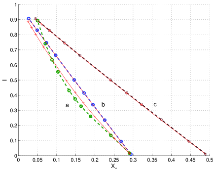
Figure 4: Current versus steady state position of the oscillator for various combination of $\eta$ and $\chi$ with varying ratio of $\gamma_{L}$ and $\gamma_{R}$ along each curve. Here we have chosen $\kappa=0.2$ a:$\eta=0.3,\chi=0.3$, b: $\eta=0.03,\chi=0.3$, c: $\eta=0.03,\chi=0.5$. Bold lines are results from the full quantum simulation and thin lines for the semiclassical approximations.

As we can see from Fig. 4(b),(c), the current is indeed linearly proportional to the steady state position of the oscillator when $\eta$ small. In this case, the semiclassical expression of the current given above in Eq. (46) is a very good approximation of the actual current.

IV A position transducer scenario

In this section, for simplicity, we assume that the zero temperature limit applies for which bound state of the dot is well below the Fermi level in the source and well above the Fermi level in the drain. The irreversible dynamics are then conveniently described in terms of two conditional Poisson jump processes with rates defined in Eqs.(14,15). The jump process Eq.(14) can only occur if there are no electrons on the dot, and the jump process Eq.(15) can only occur if there is an electron on the dot. In the case that there is no electron on the dot, the quantum dot moves in a quadratic potential centered on the origin. In the case that there is an electron on the dot, the non-zero electrostatic force means the quantum dot oscillates in a quadratic potential displaced from the origin by $X_{0}=\chi/\nu$. We thus have a picture of a system moving on one or the other potential surfaces interrupted by jumps between them. This is schematically illustrated in Fig.5. Due to the exponential dependance of the jump rates on position (see Eqs.14 and 15), the process $dN_{L}(t)$ is vastly more likely to occur when $X<0$ and conversely, the jump process $dN_{R}(t)$ is much more likely to occur when $X>0$. This means that the jump processes are an indication of which side of $X=0$ the dot is located.

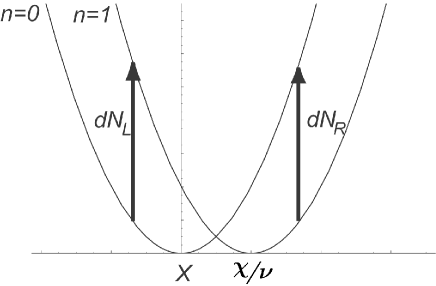
Figure 5: A schematic illustration of the two potential surfaces connected by Poisson jumps.

With this interpretation we can easily describe the conditional dynamics of the shuttle conditioned on a history of jump processes. In quantum optics such conditional dynamics are called quantum trajectoriesmolmer ; carmichael_open . Let us suppose that at time $t=t_{k}$ , the occupation of the dot is zero and the jump process $dN_{L}(t)$ occurs at $t=t_{k}+dt_{k}$. The dot then becomes occupied while the state of the oscillator changes according to gardiner-zoller

$$|\psi(t_{k})\rangle\stackrel{{\scriptstyle dN_{L}}}{{\rightarrow}}|\psi_{L}(t_{k}+dt_{k})\rangle=\frac{1}{\sqrt{p_{L}(\mu,t_{k})}}e^{-\mu\hat{x}/2}|\psi(t_{k})\rangle$$ (47)

where $p_{L}(\mu,t_{k})=\langle\psi(t_{k})|e^{-\mu\hat{x}}|\psi(t_{k})\rangle$ and we have defined $\mu=2/\lambda$. With these definitions we see that ${\cal E}(dN_{L}(t_{k}))=\gamma_{L}p_{L}(\mu,t_{k})dt$. We can develop some useful insight into what this state transformation means in the case that $|\psi(t_{k})\rangle$ is a Gaussian with mean position of $\bar{x}_{k}$ and variance $\sigma_{k}$. In this Gaussian case we have

$$p_{L}(\mu,t_{k})=e^{-\mu\bar{x}_{k}}\sum_{m=0}^{\infty}\frac{(\sigma_{k}\mu^{2})^{m}}{(2m)!}$$ (48)

where $(2m)!=2.4.6....2m$. After the jump process the mean position changes to

$$\langle\psi_{L}|\hat{x}|\psi_{L}\rangle=\bar{x}_{k}-2\sigma_{k}/\lambda.$$ (49)

This equation applies equally well to jumps to the right, $dN_{R}$, with a change in the sign of $\lambda$. Thus we see that if there is jump due to $dN_{L}$, on average the conditional state moves to state with a mean closer to the source, while if a jump occurs to the right, $dN_{R}$, the conditional state changes to a state with a mean position closer to the drain. This conditional behaviour is consistent with the interpretation of the jumps as effective measurements of the position of the quantum dot. More discussions on the quantum trajectory picture and numerical simulations on the conditional dynamics will be presented in the next section.

V Solving master equation numerically

With the help of the Quantum Optics toolbox qotoolbox , we can solve the master equation directly by finding the time evolution of the density matrix. This was done by preparing the Liouvillian matrix in Matlab and solving the differential equation given the initial conditions.

The expectation values for any desired quantities such as the electron number $\langle c^{\dagger}c\rangle$, the phonon number$\langle a^{\dagger}a\rangle$, position $\langle x\rangle$ and the momentum $\langle p\rangle$ of the oscillator can be calculated by tracing the product of this quantities with density matrix $\rho$. The result can then be plotted against time. The same method can be applied to calculate the steady state solution of the expectation values using $\rho_{ss}$.

The initial state of the system has been set up to incorporate the two electron levels, namely the occupied and empty state, combined with an $N$ levels of phonon. The number of phonon levels included determines the accuracy of the calculation. Of course the more phonon levels included the more accurate the simulation will be. However only a limited number of phonon levels can be considered. This is due to the limited computer memory that is available and also considering the calculation time which will be significantly higher for larger $N$. Thus we try to find the minimum number of phonon levels which gives convergent results. This will ensure that the simulation still has a reasonably accurate solution. Donarini donarini use the Arnoldi iterationgolub to find the stationary solution of the matrix to overcome this memory problem. However here we have proceeded without, in the hope of looking at not only the stationary solution but also the dynamical evolution of the shuttle.

The behaviour of the shuttle depends strongly on the rate of electron jump between the island and the leads. We investigate this by looking at the variation in the electron number expectation $\langle c^{\dagger}c\rangle$ at various rates $\gamma_{L},\gamma_{R}$. This is shown in Fig.
reffig:3DVarGamma in which we have set $\gamma_{L}$ to be equal to $\gamma_{R}$. When $\gamma_{L},\gamma_{R}$ are small, the electron number slowly increases until it reaches the steady state condition. In the region where the values of $\gamma_{L},\gamma_{R}$ is close to the frequency of the island, oscillation starts to occur, and depending on the damping that was set, the electron number can reach a steady oscillation putting the system well in the oscillatory regime. When $\gamma_{L}$, $\gamma_{R}$ are very large compared to other frequency scales in the system, we will arrive at the strongly damped regime of the shuttle (see Sec. V.B), where the jump rate of the electron is fast enough to damp the oscillations in the electron occupation number of the island. Since we set $\gamma_{L}$ to be equal to $\gamma_{R}$ the steady state happens at $\mbox{$\langle c^{\dagger}c\rangle$}=0.5$.

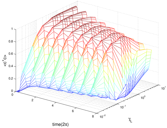
Figure 6: Plot of the electron occupation number in the island for various tunneling rate $\gamma_{L}$ in a logarithmic scale when $\eta=0.3$ $\chi=0.5$, $\nu=1$ $\kappa=0.05$.

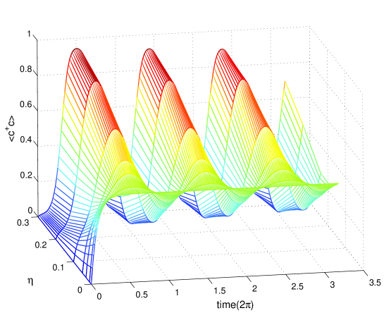
Figure 7: Plot of the electron occupation number in the island for various values of $\eta$ when $\gamma_{L}=\gamma_{R}=1$, $\chi=0.5$, $\nu=1$ $\kappa=0.05$.

Similarly the behaviour of the shuttle also changes according to $\eta$, as described in Fig.7. At $\eta=0$ the electron occupation number grows to a steady state. As we increased $\eta$ further, the oscillations start to occur with increasing amplitude. Here we use 100 phonon levels for the numerical calculation.

V.1 Oscillatory Regime

The oscillatory regime will occur when the oscillation caused by the electron jump rate introduces continued kicks on the island. This happens when the jump rate is close to the oscillation frequency of the island ($\gamma_{L}\approx\nu$). By setting an appropriate damping to this oscillation ($\kappa$), there exists a condition where the island will keep oscillating between the leads. With this setup, the system will be in the shuttle regime.

We then choose a set of parameters where the system shows the behaviour of a shuttle, that is a continued oscillation of the electron number along with the oscillation of the island position. To ensure the convergence of the numerical solution, we use a smaller value of $\eta$ that will still give a shuttling behaviour. We choose a combination of $\eta$ and $\chi$ that will give the smallest limit cycle to minimise the truncation error.

Within the region where the limit cycle exists, we can plot the electron expectation number against the average position and momentum and observe the shape of the limit cycle. We explored both the full density matrix simulation and the semiclassical solution to be compared.

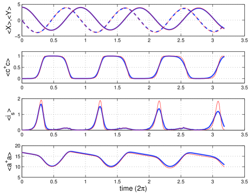
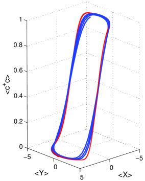
Figure 8: QO toolbox simulation for shuttling condition (bold lines), compared with the semiclassical simulation (thin lines). Parameters are $\gamma_{L}=\gamma_{R}=1,\nu=1,\eta=0.3,\chi=1,\kappa=0.05.$. We set the initial condition as $X_{0}=4.1$ and $Y_{0}=0$ to start the evolution close to the limit cycle. (a) Evolution of average values for position (solid lines) and momentum (dashed lines), electron number, current in the source and the energy of the oscillator; (b) Limit cycle behaviour in 3D.

From the result (Fig.8), the quantum simulation appears to be more damped than its semiclassical counterpart. This is due to the effect of the noise. This slight difference can also be caused by the dependence of the electron number on its correlation with the position that was ignored in the semiclassical case.

To check this we have plotted the difference between the factorized and unfactorized moment at this particular variable combination (Fig.9). The time range in which the difference in the factorized and unfactorized occurs agrees well with the time range when the semiclassical and the quantum simulation disagree in Fig.
reffig:qoshuttle. This disagreement happens at the time when the shuttle is in transition between the zero and one electron occupation number.

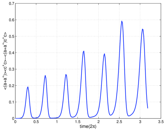
Figure 9: Plot of the difference between the factorized and unfactorized moments $\mbox{$\langle(a+a^{\dagger})\rangle$}\mbox{$\langle c^{\dagger}c\rangle$}-\mbox{$\langle(a+a^{\dagger})c^{\dagger}c\rangle$}$ in Fig.8.

Of course the truncation will pose some inaccuracy in the quantum simulation at a longer time. However we have checked that this is not the case at least for a short period of time by comparing it with a simulation that includes a larger phonon number.

To investigate the effect of $\eta$ on the correlation between the factorized and unfactorized moments, we can plot $\langle cc^{\dagger}(a+a^{\dagger})\rangle$ and $\langle cc^{\dagger}\rangle$$\langle a+a^{\dagger}\rangle$.

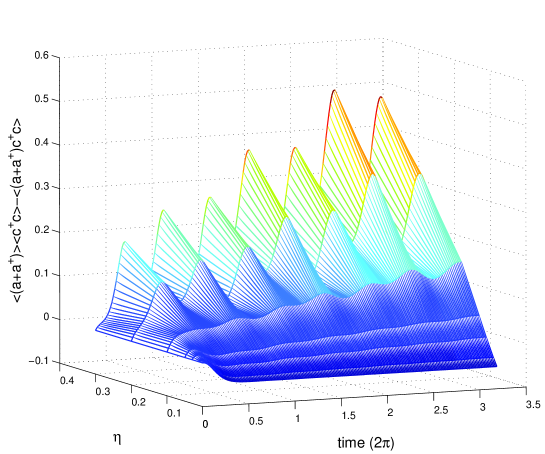
Figure 10: Plot of the difference between the factorized and unfactorized moments for various $\eta$ with $\gamma_{L}=\gamma_{R}=1,\chi=0.5,\kappa=0.05$.

We can see from Fig.10, that the semiclassical approximation agrees with the quantum simulation under the condition that $\eta$ is small enough. As $\eta$ increases, the evidence of this difference becomes noticeable. This difference oscillates with peaks located at times when electron jumps happen, that is when the oscillator is near the equilibrium position.

As opposed to what the name ”electron shuttle” suggests, the dynamics in the shuttle regime, for the parameters specified in Fig.8, is not like a conventional shuttle which picks up an electron when it is closest to the source and drops the electron when it is closest to the drain, as also suggested by Nord et al. nord . Looking at the rate of the average electron number and the average current in the source (Fig.8(a)), this is certainly not the case. The shuttle picks up an electron near an average displacement of zero, slightly towards the source, and continues to travel closer to the source electrodes. It then oscillates back and drops the electron at a slightly displaced average position from equilibrium towards the drain electrode. The shuttle then continues to get closer to the drain before oscillating back to repeat the cycle.

An important distinction must be made between the dynamics of the averages derived from solving the master equation and a dynamics conditioned on a particular history of tunneling events. This distinction is already suggested by inspecting the average electron number as a function of time. In any actual realisation of the stochastic process, the number of electrons on the dot is either zero or one, yet the ensemble average occupation number varies smoothly between zero and one. The reason for this is that the actual times at which transitions between the two states takes place fluctuates.

We can more easily appreciate this distinction using an alternative approach to understanding the dynamics based on ‘quantum trajectories’. The quantum trajectory method (sometimes called the Monte Carlo method) first introduced in quantum optics, is a method of looking at the evolution of a system conditioned on the results of measurements made on that system. dum ; carmichael_open ; goan_continuous ; goan_dynamics ; goan_montecarlo . This method will allow one to monitor ’events’ such as the jump of an electron to the island which causes the displacement kick on an oscillator.

The Quantum Optics Toolbox enables a direct computation of the conditional dynamics of the operator moments by implementing a so called ’jump unravelling’ of the master equation. First we plot a sample trajectory for a slow electron jump rate $\gamma_{L}=0.1$ to see the effect of electron jump on the evolution picture of the system. A random jump of electrons from the source to the island (Fig.11) according to rate $\gamma_{L},\gamma_{R}$ was introduced. The dynamics of the shuttle as a position transducer, as predicted in section IV, can be seen in the conditional averages of the displacement. The variable $\eta$ controls the amount of displacement of the island when an electron jumps on and off onto the island. Larger value of $\eta$ caused a larger displacement kick when a jump occurs. During the time when the electron is on the island, the phonon number of the oscillator oscillates with a similar behaviour to the oscillation of the position.

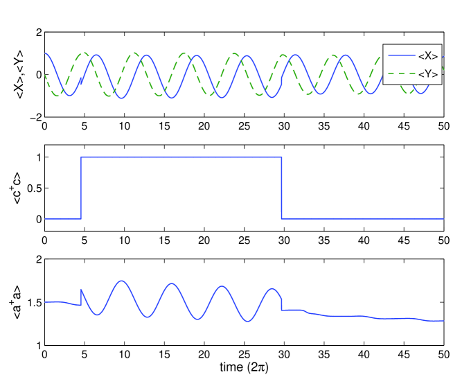
Figure 11: Plot of a single trajectory showing the dynamics of the jump and the result in the phonon number. Parameters are $\gamma_{L}=\gamma_{R}=0.1,\nu=1,\eta=0.3,\chi=1,\kappa=0.05$.

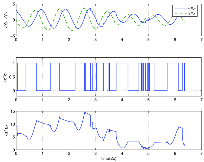
Figure 12: Plot of a single trajectory showing the dynamics of the jump when $\gamma_{L}=\gamma_{R}=1,\nu=1,\eta=0.3,\chi=1,\kappa=0.05.$

The single trajectory for the shuttle case with the same parameter in Fig.8 can be seen in Fig.12. The electrons mostly jump onto the island from the source when it is closer to the source and jump off when closer to the drain. At the jump, the island gets a slight displacement kick towards the source when jumping on and towards the drain when jumping off. However this does not stop the shuttling motion of the island and does not repel it to the opposite direction as suggested earlier by Nord et al. nord . It can also be seen that when the electron manages to jump onto the island when island is still close to the drain, it is more probable for the electron to jump off straight away.

The conditional dynamics of the system just described corresponds to an experiment in which number of electrons on island is monitored continuously in time. As we can see, the behaviour of the conditional dynamics differs from the behaviour of the ensemble average. However, averaging over many different realization of the trajectories as shown in Fig.12 would lead to a closer and closer approximation of the ensemble average behaviour in Fig.8.

V.2 Strongly Damped Regime

There are two ways of damping the shuttle into the fixed point regime. One is to damp the motion of the shuttle itself by introducing a large mechanical damping $\kappa$. Alternatively we can damp the oscillation of the electron occupation number in the island. This happens when the rates of the electron jump $\gamma_{L},\gamma_{R}$ are large compared to the natural frequency of the island vibration. The fast electron jumps act as an internal damping to the shuttle. Within this regime the electron number expectation $\langle c^{\dagger}c\rangle$ monotonically approaches 0.5 when $\gamma_{L}=\gamma_{R}$.

When the bare electron tunnelling rates are very large compared to other frequency scales in the problem, we may assume the dot approaches its steady state for bare tunnelling quickly as compared to the typical time scale of the oscillator. In this case, $\rho(t)=\rho_{d}^{\rm st}\times\rho_{o}(t)$. The bare $\rho_{d}^{\rm st}$ can be substituted into the density matrix of the total master equation and then be traced out with respect to the dot degrees of freedom to get an effective master equation which involves only the reduced density matrix of the oscillator. This effective master equation can be calculated from the reduced density matrix, from Eq. (11).

Since $\eta$ is assumed to be small, we can expand the expression to second order in $\eta$: $e^{\eta\hat{X}}=1+\eta\hat{X}+(\eta\hat{X})^{2}/(2!)+\cdots$. We can then re-write the zero temperature full master equation as:

$$\dot{\rho} = -i\nu[a^{\dagger}a,\rho]$$ (50)

$$+ 2i\chi[\hat{X}\bar{n},\rho]$$

$$+ 2\gamma_{L}(1-\bar{n})\eta^{2}[\hat{X},[\hat{X},\rho]]$$

$$+ 2\gamma_{R}\bar{n}\eta^{2}[\hat{X},[\hat{X},\rho]]$$

$$+ \kappa(\bar{n}_{p}+1)\mathcal{D}[a]\rho+\kappa\bar{n}_{p}\mathcal{D}[a^{\dagger}]\rho,$$

with $\bar{n}=\gamma_{L}/\gamma_{L}+\gamma_{R}$. The following moments can thus be derived from Eq. (50):

$$\frac{d\mbox{$\langle a^{\dagger}a\rangle$}}{dt} = 2\chi\bar{n}\mbox{$\langle\hat{Y}\rangle$}-4\gamma_{L}(1-\bar{n})\eta^{2}-4\gamma_{R}\bar{n}\eta^{2}+\kappa\bar{n}-\kappa\mbox{$\langle a^{\dagger}a\rangle$}$$ (51)

$$\frac{d\mbox{$\langle\hat{X}\rangle$}}{dt} = \nu\mbox{$\langle\hat{Y}\rangle$}-\frac{\kappa}{2}\mbox{$\langle\hat{X}\rangle$}$$ (52)

$$\frac{d\mbox{$\langle\hat{Y}\rangle$}}{dt} = -\nu\mbox{$\langle\hat{X}\rangle$}+\chi\bar{n}-\frac{\kappa}{2}\mbox{$\langle\hat{Y}\rangle$}.$$ (53)

The moments $\langle\hat{X}\rangle$ and $\langle\hat{Y}\rangle$ form a closed system of differential equation which can readily be solved.

$$\langle\hat{X}\rangle = e^{-(\kappa/2)t}\biggl{(}(X_{0}-X_{*})\cos(\nu t)+(Y_{0}-Y_{*})\sin(\nu t)\biggr{)}+X_{*},$$ (54)

$$\langle\hat{Y}\rangle = e^{-(\kappa/2)t}\biggl{(}-(X_{0}-X_{*})\sin(\nu t)+(Y_{0}-Y_{*})\cos(\nu t)\biggr{)}+Y_{*}.$$ (55)

where again $X_{*}$ and $Y_{*}$ is simply the displacement in the equilibrium such as given in Eqs.(32) and (33) with $n_{*}=\bar{n}$. $X_{0}$ and $Y_{0}$ is the initial condition of $X$ and $Y$ respectively. The analytic expressions of Eqs.(54) and (55) are useful for checking the solution of the master equation given by Matlab, to ensure that the truncation in the phonon number is adequate.

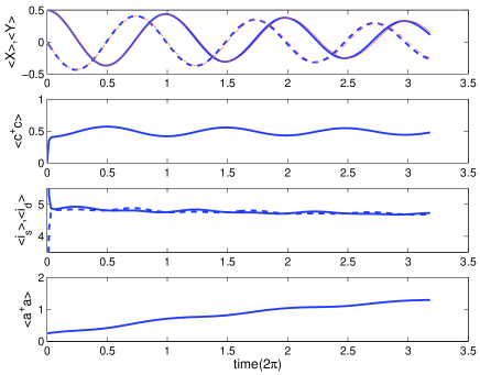
Figure 13: Average evolution of the shuttle with a large $\gamma_{L}$ and $\gamma_{R}$. Here we have chosen $\gamma_{L}=\gamma_{R}=10,\eta=0.1,\chi=0.1,\kappa=0.05,X_{0}=0.5,Y_{0}=0$ for both quantum simulation with $N=25$ (thick lines) and semiclassical solution (thin lines).

The shuttle oscillation is damped to the new displaced position of $X_{*}$ which agrees to the obtained result previously. When $\gamma_{L}=\gamma_{R}=gamma$, we have $n_{*}=\bar{n}=\mbox{$\frac{1}{2}$}$ in the regime when the tunneling rates are very large compared to other frequency scales (especially when $\eta$ is relatively small). In this case, the oscillatory behaviour of Eqs. (54) and (55) do not depend on the actual values of the tunneling rates $gamma$. It can also be deduced that the decay rate of the oscillation envelope is $e^{-\kappa t/2}$. In this regime, the result of the analytical expressions matches the quantum simulation quite well.

V.3 Co-existence regime

As discussed in Sec. III, we can also have a regime in which the behaviour of the shuttle depends on its initial condition. The system will either be attracted to the limit cycle and thus be in the shuttle regime or be attracted to the fixed point and be in the tunneling regime depending on its initial condition within the correct parameters where the subcritical bifurcation occurs. Following previous authorsdonarini , we call this the ’co-existence regime’.

Semiclassically this can be seen when we plot the average evolution of the shuttle. Depending on the initial conditions, the shuttle will either be attracted to the fixed point position or undergoes the stable limit cycle oscillation (Fig. 14).

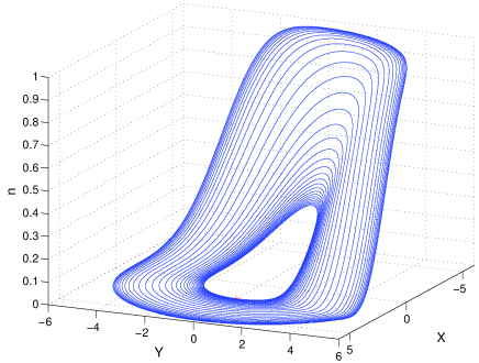
Figure 14: Semiclassical limit cycle of the shuttle in the co-existence regime. Here we have chosen $\gamma_{L}=0.03,\gamma_{R}=1,\eta=0.3,\chi=1,\kappa=0.05,X_{0}=2.2$ and $Y_{0}=0$. The evolution starts close to the unstable limit cycle and then moves toward the stable limit cycle

The quantum average calculation in this regime however does not show the subcritical bifurcation since averaging over the noise in the system dampens this effect. This can be seen in the evolution of the single trajectory which is captured to the fixed point position at random times. A sample of trajectories each from different initial conditions were plotted in figure 15 and 16.

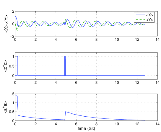
Figure 15: Average evolution of the shuttle. Here we have chosen $\gamma_{L}=0.01,\gamma_{R}=1,\eta=0.3,\chi=1,\kappa=0.05,X_{0}=1.2,Y_{0}=0$.

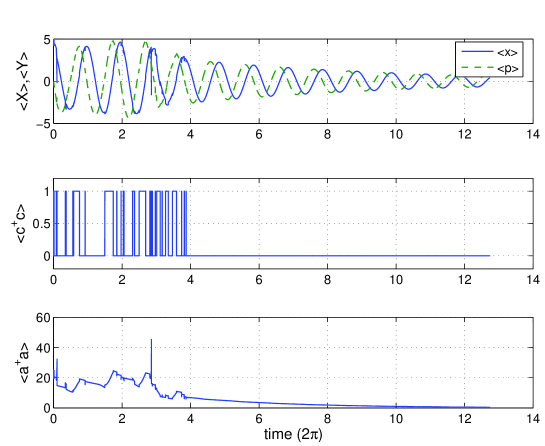
Figure 16: Average evolution of the shuttle. Here we have chosen $\gamma_{L}=0.01,\gamma_{R}=1,\eta=0.3,\chi=1,\kappa=0.05,X_{0}=5,Y_{0}=0$.

V.4 Finite Temperature

We can easily extend these calculations to the finite temperature case by including the fermi factor $f_{L}$ and $f_{R}$, which was previously set to 1 and 0 for the zero temperature case, in the calculation for both the full quantum simulation and the semiclassical approximation.

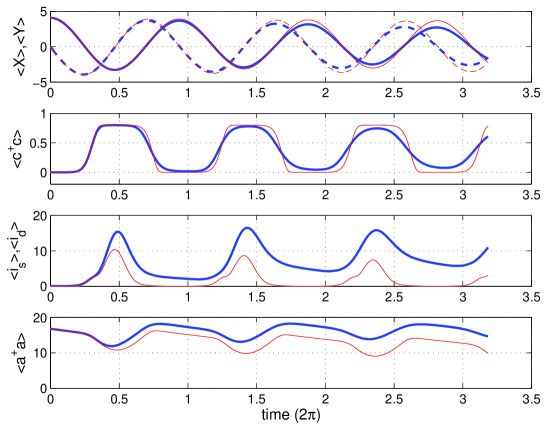
Figure 17: Average evolution of the shuttle with finite Temperature $\gamma_{L}$ and $\gamma_{R}$. Here we have chosen $\gamma_{L}=\gamma_{R}=1,\eta=0.3,\chi=1,\kappa=0.05,X_{0}=4.1,Y_{0}=0,f_{L}=0.8$ and $f_{R}=0$ at $\omega_{I}=3\nu$ for both quantum simulation with $N=47$ (thick lines) and semiclassical approximation (thin lines).

The effect on temperature on the system is shown in Fig. 17. Comparing this with previous result for the zero temperature (Fig. 8) there is a suppression of the electron number oscillation. There is also a significant difference between the quantum and the semiclassical simulation for the electron number occupation which resulted in a difference in the current in each of the leads.

VI Noise calculation

In surface gated 2DEG structures some recent experiments monitor the charging state of the dot via conductance in a quantum point contactkouwenhoven . However such techniques cannot easily be adapted for a nanoelectromechanical system. In experiments involving tunneling through a double barrier quantum dot structure the simplest thing to measure is the source-drain current. In the QEMS experiments of Park et alpark and also of Erbe et al, the source drain current carried signatures of the vibration of the nanoelectromechanical component. In this section we calculate, using the Quantum Optics Toolbox, the current noise spectrum and show that it indicates the transition between the fixed point and the shuttling regime.

The current seen in the external circuit, when electrons tunnel on and off the dot, only indirectly reflects the quantum nature of the tunneling process. Tunneling causes a local departure from equilibrium in the source and drain reservoirs that is restored through a fast irreversible process in which small increments of charge are exchanged with the external circuit. While tunneling obviously involves a change of charge in units of $\pm$e, the increments of charge drawn by the external circuit are continuous quantities determined by the overall capacitance and resistance of the circuit. The current responds as a classical stochastic process conditioned on the quantum stochastic processes involved in the tunneling. In many ways this is analogous to the response of a photo electron detector to photons.

The connection between the quantum stochastic process of tunneling and the current observed in the external circuit is given by the Ramo-Shockley theorem and is a linear combination of the two Poisson processes defined in Eqs. (14,15). The noise spectrum of such a current involves moments of both the tunneling processes, and correlations between them. In Sun et al.sun , one can find a detailed example of how such correlations are determined by the corresponding master equation for the quantum dot system.

Recently Flindt et al.flindt , have calculated a noise spectrum for the shuttle system defined in terms of the fluctuating electron number accumulating in the drain reservoir. Here we adopt a different (but equivalent) approach based on the framework of quantum trajectories. In this section we calculate, using quantum trajectory methods, the stationary current noise spectrum in the source current alone as this suffices to illustrate how the current noise spectrum reflects the transition from fixed point to shuttling. The total current shows the same features but has a different noise background.

The two time correlation function quantifies the fluctuations in the observed current and is defined by:

$$G(\tau)=\frac{e}{2}i_{\infty}\delta(\tau)+E(I(t)I(t+\tau))^{\tau\neq 0}_{t\rightarrow\infty},$$

The first term is responsible for shot noise in the current, while the second term quantifies noise correlations. We now show how the second term can be defined in terms of the stationary state of the quantum dot itself.

Let $\rho(t)$ be the density operator representing the dot at time $t$. What is the conditional probability that, given an electron tunnels onto the dot from the drain between $t$ and $t+dt$, another similar tunneling event takes place a time $\tau$ later (with no regard for what tunneling events have occurred in the mean time)? If an electron tunnels onto the dot from the drain at time $t$, the conditional state of the dot (unnormalised), conditioned on this event is given by

$$\tilde{\rho}^{(1)}(t)=\gamma_{L}e^{-\hat{x}/\lambda}c^{\dagger}\rho(t)ce^{-\hat{x}/\lambda}.$$ (56)

Given this state, the probability that another tunneling event takes place a time $\tau$ later is

$$G(t,\tau) = \gamma_{L}{\rm tr}\left(e^{-2\hat{x}/\lambda}cc^{\dagger}e^{{\cal L}\tau}[\tilde{\rho}^{(1)}(t)]\right)$$

$$= \gamma^{2}_{L}{\rm tr}\left(e^{-2\hat{x}/\lambda}cc^{\dagger}e^{{\cal L}\tau}[e^{-\hat{x}/\lambda}c^{\dagger}\rho(t)ce^{-\hat{x}/\lambda}]\right).$$

where formally we have represented the irreversible dynamics from time $t$ to $t+\tau$ as the propagator $e^{{\cal L}\tau}$. Let us now assume that the first conditioning event takes place at a time $t$ long after any information about the initial state of the quantum dot has decayed away. That is to say the first conditioning event occurs when the dot has settled into the stationary state, $\rho_{\infty}=\lim_{t\rightarrow\infty}\rho(t)$. The stationary two-time correlation function for the source current is then defined by

$$G(\tau)=\gamma^{2}_{L}{\rm tr}\left(e^{-2\hat{x}/\lambda}cc^{\dagger}e^{{\cal L}\tau}[e^{-\hat{x}/\lambda}c^{\dagger}\rho_{\infty}ce^{-\hat{x}/\lambda}]\right)$$ (57)

In terms of the dimensionless position operator, $X$, the noise in the two time correlation functions becomes

$$G(\tau)=E(I_{L}(t)I_{L}(t+\tau))^{\tau>0}_{t\to\infty}=\gamma_{L}^{2}{\rm Tr}[e^{-4\eta\hat{X}}cc^{\dagger}e^{{\cal L}\tau}(e^{-2\eta\hat{X}}c^{\dagger}\rho_{\infty}ce^{-2\eta\hat{X}})]$$

where $e^{{\cal L}\tau}$ is the master equation evolution.

The noise power spectrum of the current is given by:

$$S(\omega)=2\int_{0}^{\infty}G(\tau)(e^{i\omega\tau}+e^{-i\omega\tau})d\tau$$ (58)

This noise spectrum can be directly calculated using the Quantum Optics Toolbox by first calculating the steady state solution $\rho_{\infty}$ and setting $e^{-2\eta\hat{X}}c^{\dagger}\rho_{\infty}ce^{-2\eta\hat{X}}$ as an initial condition for the master equation evolution. Then we can calculate the expectation value of the operator $cc^{\dagger}e^{-4\eta\hat{X}}$ in the state evolved, according to the master equation, from this initial condition. It is important to note that the master equation does indeed have a steady state even in that parameter regime in which the semiclassical dynamics would imply a limit cycle. This is because quantum fluctuations cause a kind of phase diffusion around the limit cycle. These quantum fluctuations are precisely the random switchings observed in the single quantum trajectory shown in figure 12. In fact as shown in novotny the Wigner function of the steady state has support on the entire limit cycle.

The example of the noise spectra for various $\eta$ is shown in Fig.18.

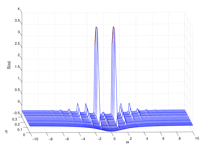
Figure 18: Plot of spectrum in the left junction with various $\eta$, setting $\chi=0.5$.

The transition between the tunnelling regime and the shuttling regime is clearly evident in the noise power spectrum, figure 18 (We have subtracted off the shot noise background).

Setting $\eta=0,\chi=0$ we arrived back at the known spectrum for the source current in a double barrier devicesun with a single dip at zero frequency. As the values of $\eta$ and $\chi$ (or $\gamma_{L}$) are increased, the frequency spectra develop sidebands which correspond to the frequency of the oscillator (Fig.
reffig:corrspectrum,19). As the system approaches the shuttling regime, the frequency spectra pick up noise peak at zero frequency and additional peaks at higher frequencies close to a multiple of the oscillator frequency. This is a signature of the limit cycle formation. On the limit cycle, the frequency is shifted from the base oscillation frequency $\omega=1.055\nu$. This is also given by the imaginary part of the eigenvalues of the linearised matrix expressed $\mu=\sqrt{A_{*}\kappa+1+(\kappa/2)^{2}}$. This observation agrees with the predicted slight re-normalization of the frequency by Flindt et al. flindt .

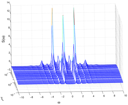
Figure 19: Plot of spectrum in the left junction with various $\gamma_{L}$, setting $\eta=0.3,\chi=0.5,\kappa=0.05.$

A similar feature of the noise is found by Armour armour_current in a system consisting of a SET that is coupled to a nanomechanical resonator. Although this is a different system from the shuttle system, the classical spectrum noise in this system also shows the dependency of the current on the position of the nanomechanical resonator.

VII Conclusion

The dynamics of the shuttle system has been investigated via both the semi-classical and the full quantum master equation treatment. The latter reveals subtle properties of the dynamics which was not found using the semiclassical treatment. The master equation is solved numerically using the Quantum Optics Toolbox enabling a detailed comparison of the semiclassical dynamics with the quantum ensemble averages. For the first time in the study of the quantum shuttle we compute the moments for the quantum state conditioned on a particular history of tunnelling events. This is called a quantum trajectory and it reflects what can be observed experimentally by monitoring the electron on the island.

The conditional dynamics differs from the behaviour of the ensemble average, and gives new insight into the shuttling dynamics. In the shuttling regime, the ensemble average dynamics of the electron occupation number is a smoothed square wave that slowly decays to a steady state value of one half. Given that the occupation number of the dot is either zero or unity this ensemble averaged behaviour may seem unexpected. However looking at the occupation number in a single conditional state (see Fig. 11) indicates what is going on. A single quantum trajectory shows that the average occupation number is indeed either zero or unity and in the shuttling regime behaves like a square wave for short times but, at random times, suffers a phase jump. The ensemble average of many such trajectories with phase jumps at random times leads to the observed ensemble average dynamics as computed from the master equation. These random phase jumps ultimately lead to a steady state density operator for the system that, in the Wigner representation, is diffused around the limit cycle, as noted by Novotny et al.novotny .

The shuttle dynamics was investigated in two regimes: the fixed point and the shuttle regime. In the fixed point regime, the shuttle is damped to a new displaced position. We have shown that there is a strong relation between the current and the fixed point of the position. This relationship is linear when the tunnel length is large ($\eta$ small). Thus it is possible to use the shuttle in a position transducer scenario. In this regime, the semiclassical treatment is shown to be accurately sufficient to describe the dynamics.

We provide the condition in which the shuttle regime will appear from the system by identifying the appearance of limit cycle in the phase space of the shuttle. A careful analysis of the nonlinear dynamics using centre manifold method indicates that when $\gamma_{L}=\gamma_{R}$, the limit cycle forms through a supercritical pitchfork bifurcation. However when $\gamma_{L}\neq\gamma_{R}$ there is a region of parameter space in which the bifurcation can be subcritical, and for which hysteresis is possible. Adjusting the damping $\kappa$ with respect to these parameters will cause the shuttle to be sufficiently damped and thus allow the shuttling to take place. The shuttle regime also appears when the rate of the electron tunnelling is close to the oscillator frequency. The shuttle regime corresponds to the continuous oscillation of the electron number and results in additional peaks at multiples of the limit cycle frequency in the noise spectra. This is destroyed when $\kappa$ is too large or when a large electron jump $\gamma_{L},\gamma_{R}$ are introduced to the system. Both of these conditions will damp the shuttle into the displaced equilibrium position. The quantum shuttle thus provides a fascinating example of a quantum stochastic system in which electron transport is coupled to mechanical motion. In future studies we will investigate how such a system can be configured for sensitive force detection.

References

- (1) R. G. Knobel and A. N. Cleland, Nature 424, 291 (2003).
- (2) M. D. LaHaye, O. Buu, B. Camarota, and K. Schwab, Science 304, 74 (2004).
- (3) K. L. Ekinci, X. M. H. Huang, and M. L. Roukes, Appl. Phys. Lett. 84, 4469 (2004).
- (4) L. Gorelik et al., Phys. Rev. Lett. 80, 4526 (1998).
- (5) S. Tan, Quantum Optics Toolbox, http://www.phy.auckland.ac.nz/Staff/smt/qotoolbox/download.html.
- (6) K. Molmer, Y. Castin, and J. Dalibard, Journal of the Optical Society of America B (Optical Physics) 10, 524 (1993).
- (7) R. I. Shekhter et al., J. Phys.: Condens. Matter 15, R441 (2003).
- (8) H. Park et al., Nature 407, 57 (2000).
- (9) N. Zhitenev, H. Meng, and Z. Bao, Phys. Rev. Lett. 88, 226801 (2002).
- (10) A. Erbe, C. Weiss, W. Zwerger, and R. Blick, Phys. Rev. Lett. 87, 096106 (2001).
- (11) X. M. H. Huang, C. A. Zorman, M. Mehregany, and M. L. Roukes, Nature 421, 496 (2003).
- (12) A. Isacsson and T. Nord, Europhys. Lett. 66, 708 (2004).
- (13) T. Novotny, A. Donarini, C. Flindt, and A.-P. Jauho, Phys. Rev. Lett 92, 248302 (2004).
- (14) C. Flindt, T. Novotny, and A.-P. Jauho, Physica E 28, in press (2005).
- (15) A. Isacsson, Phys. Rev. B 64, 035326 (2001).
- (16) A. Donarini, cond-mat/0501242 v1, 2005.
- (17) V. Aji, J. E. Moore, and C. M. Varma, APS Meeting Abstracts 17004 (2003).
- (18) K. D. McCarthy, N. Prokof’ev, and M. T. Tuominen, Phys. Rev. B 67, 245415 (2003).
- (19) D. Fedorets, L. Gorelik, R. Shekhter, and M. Jonson, Phys. Rev. Lett 92, 166801 (2004).
- (20) T. Novotny, A. Donarini, and A.-P. Jauho, Phys. Rev. Lett. 90, 256801 (2003).
- (21) A.-P. Jauho, T. Novotny, A. Donarini, and C. Flindt, cond-mat/0411107 v1 .
- (22) A. Armour and A. MacKinnon, Phys. Rev. B 66, 035333 (2002).
- (23) C. W. Gardiner and P. Zoller, Quantum Noise, 2nd ed. (Springer-Verlag, Berlin, 2000).
- (24) D. W. Utami, H.-S. Goan, and G. J. Milburn, Phys. Rev. B 70, 075303 (2004).
- (25) H.-S. Goan, G. J. Milburn, H. M. Wiseman, and H. B. Sun, Phys. Rev. B 63, 125326 (2001).
- (26) H.-S. Goan and G. J. Milburn, Phys. Rev. B 64, 235307 (2001).
- (27) H.-S. Goan, Phys. Rev. B 72, 075305 (2005).
- (28) P. Glendinning, Stability, instability and chaos: an introduction to the theory of nonlinear differential equations (Cambridge University Press, New York, 1994).
- (29) H. J. Carmichael, An open systems approach to quantum optics (Springer-Verlag, Berlin, Heidelberg, 1993).
- (30) G. H. Golub and C. F. Loan, Matrix Computations, 3rd ed. (The John Hopkins University Press, Baltimore, Maryland 21218, USA, 1996).
- (31) T. Nord, L. Gorelik, R. Shekhter, and M.Jonson, Phys. Rev. B 65, 165312 (2002).
- (32) R. Dum, P. Zoller, and H. Ritsch, Phys. Rev. A 45, 4879 (1992).
- (33) J. M. Elzerman et al., Nature 403, 431 (2004).
- (34) H. B. Sun and G. Milburn, Phys. Rev. B 59, 10748 (1999).
- (35) A. Armour, Phys. Rev. B 70, 165315 (2004).