High-precision finite-size scaling analysis of the quantum-critical
point of S = 1/2 Heisenberg antiferromagnetic bilayers

Abstract

We use quantum Monte Carlo (stochastic series expansion) and finite-size scaling to study the quantum critical points of two $S=1/2$ Heisenberg antiferromagnets in two dimensions: a bilayer and a Kondo-lattice-like system (incomplete bilayer), each with intra- and inter-plane couplings $J$ and $J_{\perp}$. We discuss the ground-state finite-size scaling properties of three different quantities—the Binder moment ratio, the spin stiffness, and the long-wavelength magnetic susceptibility—which we use to extract the critical value of the coupling ratio $g=J_{\perp}/J$. The individual estimates of $g_{\text{c}}$ are consistent provided that subleading finite-size corrections are properly taken into account. In the case of the complete bilayer, the Binder ratio leads to the most precise estimate of the critical coupling, although the subleading finite-size corrections to the stiffness are considerably smaller. For the incomplete bilayer, the subleading corrections to the stiffness are extremely small, and this quantity then gives the best estimate of the critical point. Contrary to predictions, we do not find a universal prefactor of the $\sim 1/L$ spin stiffness scaling at the critical point, whereas the Binder ratio is consistent with a universal value. Our results for the critical coupling ratios are $g_{\text{c}}=2.52181(3)$ (full bilayer) and $g_{\text{c}}=1.38882(2)$ (incomplete bilayer), which represent improvements of two orders of magnitude relative to the previous best estimates. For the correlation length exponent we obtain $\nu=0.7106(9)$, consistent with the expected 3D Heisenberg universality class.

I Introduction

The two-dimensional (2D) $S=1/2$ Heisenberg antiferromagnet has received considerable attention in the past two decades because of its close relation to the CuO₂ layers of the cuprate superconductors.ManousakisRMP1990 Other, even better realizations of this model system have been discovered as well. RonnowPRL2001 The properties of the single-layer Heisenberg model have been thoroughly studied using both analytical and numerical methods, and there is very good agreement with experiments, e.g., for the temperature dependence of the spin correlation length ChakravartyPRL1988 ; KimPRL1998 in La₂CuO₄ (measured using neutron scattering) and NMR relaxation rates.SandvikPRB1995

Mapping the lattice Heisenberg model onto a continuum field theory yields the (2+1)-dimensional nonlinear sigma-model,HaldanePRL1983 ; ChakravartyPRL1988 the coupling constant $g$ of which controls the transition from Néel order to quantum disorder at temperature $T=0$ (quantum phase transition SachdevBOOK1999 ). This transition is in the universality class of the finite-$T$ transition of the 3D classical Heisenberg model. ChakravartyPRL1988 ; HaldanePRL1988 Having an ordered ground state, RegerPRB1988 the 2D square-lattice $S=1/2$ Heisenberg model corresponds to $g<g_{\text{c}}$. Even so, there is some influence from the critical point, because a quantum phase transition is also associated with universal quantum critical scaling at finite temperature, in an extended ($g,T$) regime where temperature is the dominant energy scale.ChubukovPRB1994 The energy scales characterizing the ordered and disordered phases—the spin stiffness and the singlet-triplet gap, respectively—vanish continuously as $g\to g_{\text{c}}$, and hence the quantum critical regime fans out from the point $(g=g_{\text{c}},T=0)$.

A quantum phase transition of the type described by the nonlinear sigma-model can be realized in the Heisenberg antiferromagnet by introducing a pattern of two (or more) different coupling strengths in a way that favors singlet formation on dimers (or larger units of an even number of spins). ChakravartyPRL1988 ; ChubukovPRB1994 This leads to an order-disorder transition at some critical coupling ratio. Models of this kind, e.g., a bilayer where dimers form across the layers,HidaJPSJ1990 ; MillisPRL1993 ; SandvikPRL1994 single layers with various dimer patterns,SinghPRL1988 or a regularly depleted system where singlets form on rings of four or eight spins,TroyerPRL1996 have been extensively studied using quantum Monte Carlo simulations in order to confirm the expected universality class and to test very detailed predictions ChubukovPRB1994 of the finite-$T$ quantum critical behavior of various quantities. The predicted universal behavior was confirmed at low temperature. SandvikPRL1994 ; ShevchenkoPRB2000 ; TroyerPRL1996 ; BrenigCM2005 The simulations also served to establish the onset of nonuniversal lattice effects at higher temperature and the nature of the cross-over ChubukovPRB1994 to the low-temperature renormalized classical or quantum-disordered regimes away from the critical point.

In this paper we study the critical points of two different $S=1/2$ Heisenberg models: a symmetric bilayer and a Kondo-lattice-like system in which there are no intra-plane couplings in one of the layers. We will refer to these systems as the full and incomplete bilayers, respectively; see Fig. 1. Their Hamiltonians ($H_{1}$ for the full bilayer and $H_{2}$ for the incomplete bilayer) are given by

$$H_{1} =J\sum_{\langle i,j\rangle}\bigl{(}{\bf S}_{1i}\cdot{\bf S}_{1j}+{\bf S}_{2i}\cdot{\bf S}_{2j}\bigr{)}+J_{\perp}\sum_{i}{\bf S}_{1i}\cdot{\bf S}_{2i},$$ (1)

$$H_{2} =J\sum_{\langle i,j\rangle}{\bf S}_{1i}\cdot{\bf S}_{1j}+J_{\perp}\sum_{i}{\bf S}_{1i}\cdot{\bf S}_{2i}.$$ (2)

Here, ${\bf S}_{a,i}$ is a spin-1/2 operator at site $i$ of layer $a$ ($a=1,2$), and $\langle i,j\rangle$ denotes a pair of nearest-neighbor sites on the square lattice of $L\times L$ sites with periodic boundary conditions. Both coupling constants are antiferromagnetic ($J,J_{\perp}>0$). In order to avoid any frustration we consider only even $L$. As the ratio $g=J_{\perp}/J$ is increased, there is a tendency to form inter-plane near-neighbor singlets, which at some $g=g_{\text{c}}$ leads to the opening of a spin gap and destruction of the long-range Néel order present for $g<g_{\text{c}}$ (in the limit $g\to\infty$ the ground state is a singlet product, which clearly cannot support long-range spin-spin correlations). This is the transition we investigate in detail in this paper.

Figure 1: The arrangement of spin interactions in the (a) full and (b) incomplete bilayers. There are two different couplings: $J$ (intra-plane) and $J_{\perp}$ (inter-plane), as indicated.

Our purpose in studying these models is two-fold. First, we would like to determinate the locations of the critical points to much higher accuracy than they are currently known. The best estimates to date are $g_{\text{c}}=2.525(2)$ (full bilayer) ShevchenkoPRB2000 and $g_{\text{c}}=1.393(8)$ (incomplete bilayer) KotovPRL98 (see also Ref. BrenigCM2005, ). The statistical accuracies here are quite modest compared to results for the standard classical critical points (e.g., the 3D Heisenberg model HolmPRB1993 ; CompostriniPRB2002 ). It would be useful to increase the precision so that studies of various aspects of finite-$T$ quantum criticality (e.g., interesting properties of isolated impurities in a critical host system SachdevSCI1999 ; TroyerPTP2002 ; SachdevPRB2003 ; SushkovPRB2003 ; HoglundUNP ) could be studied numerically at low $T$ very close to the critical point (minimizing the effects of the eventual cross-over to the renormalized-classical or quantum-diosrdered regime). Second, we wish to compare several different ways of extracting the critical coupling, in order to gain additional confidence in the results and to provide guidance for studies of other quantum critical points. The reason for choosing the particular bilayer lattices of Fig. 1 over other 2D Heisenberg systems undergoing the same type of transition is that they do not break any in-plane symmetries of the square lattice.

We have carried out finite-size scaling of low-temperature ($T\to 0$ converged) QMC results for three different quantities: the spin stiffness, the Binder cumulant ratio, and the long-wavelength (uniform) magnetic susceptibility. We use our recently proposed method for including subleading finite-size corrections.KevinPRE05 Although this necessitates nonlinear fits with a relatively large number of independent parameters, we believe that this is necessary in order to obtain completely unbiased results. Our final results for the critical couplings are $g_{\text{c}}=2.52181(3)$ for the full bilayer and $g_{\text{c}}=1.38882(2)$ for the incomplete bilayer, i.e., the statistical precision is improved by approximately two orders of magnitude relative to the previous estimates. Our fitting procedure also gives the correlation-length exponent $\nu$, but because of the multi-parameter fits and the relatively modest lattices sizes ($L$ up to $42$), its statistical precision is not quite as high (the error bars are roughly twice as large) as that of recent classical Monte Carlo simulations of the 3D Heisenberg model.CompostriniPRB2002 Nevertheless, our result, $\nu=0.7106(9)$, is fully consistent with the presently most accurate value of this exponent, $\nu=0.7112(5)$. CompostriniPRB2002

We also discuss the universality of the Binder moment ratio and the spin stiffness at the critical point. In the former case, we point out a difference relative to classical systems in how the order-parameter moments are defined and calculated, and in the latter case we do not find the universality that has been suggested for the prefactor of the $\sim 1/L$ scalingWallinPRB1994 (i.e., we obtain different prefactors for the two different bilayer models).

The rest of the paper is organized as follows. In Sec. II we discuss the quantities that we have calculated and their QMC (Stochastic Series Expansion, SSE) estimators, as well as their expected finite-size scaling forms. In Sec. III we first briefly review our approach to deal with subleading finite-size corrections and then present the results of the analysis. We give a brief summary and conclusions in Sec. IV.

II Calculated observables and their critical scaling properties

We have used the SSE QMC method with operator-loop updates.SandvikPRB1999 This approach is based on sampling diagonal matrix elements of the power series expansion of $\exp(-\beta H)$, where $\beta$ is the inverse temperature. We use $L\times L\times 2$ lattices with periodic boundary conditions in the $x$ and $y$ directions, with even $L$ up to $42$. In order to ensure convergence of all calculated quantities to their ground-state values, we carried out simulations at inverse temperatures $\beta_{n}=2^{n}$ with integer $n$ taken large enough so that results for $\beta_{n}$ and $\beta_{n-1}$ agree within statistical errors. Examples of the convergence are shown in Fig. 2.

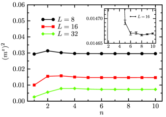
Figure 2: (Color online) Convergence as a function of inverse temperature $\beta=2^{n}$ of the squared sublattice magnetization to its ground state value for three different lattice sizes.

II.1 Binder Moment Ratios $Q_{k}$

The magnetic moment ratios $Q_{k}$ introduced by Binder BinderPRL1981 have the very useful property of being universal at the critical point, because all nonuniversal scale factors cancel out along with the length dependence. This follows from the finite-size scaling hypothesis for the ordered moment (here the staggered magnetization). The $k^{\text{th}}$ power of the staggered magnetization scales as

$${\langle|m|^{k}\rangle}_{L}=L^{-k\beta/\nu}M_{k}(tL^{1/\nu}),$$ (3)

where $L$ is the linear system length, $\beta$ and $\nu$ are critical indices in their standard notation, and $t$ is the reduced coupling constant, which we define here in terms of the coupling ratio $g$ as $t=(g-g_{\text{c}})/g_{\text{c}}$. $M_{k}(x)$ are the scaling functions. Consequently, the moment ratios

$$Q_{k}(t,L)=\frac{{\langle m^{2k}\rangle}_{L}}{{\langle m^{2}\rangle}^{k}_{L}}$$ (4)

are dimensionless scaling functions. At the critical point, $Q_{k}(0,\infty)$ are universal constants.

We have computed the first two Binder ratios, which we define as

$$Q_{1} = \frac{\langle m^{2}\rangle}{{\langle|m|\rangle}^{2}}=\frac{3\langle(m^{z})^{2}\rangle}{2{\langle|m^{z}|\rangle}^{2}},$$ (5)

$$Q_{2} = \frac{\langle m^{4}\rangle}{{\langle m^{2}\rangle}^{2}}=\frac{5\langle(m^{z})^{4}\rangle}{3{\langle(m^{z})^{2}\rangle}^{2}},$$ (6)

where $m^{z}$ is the $z$-component of the staggered magnetization operator,

$$m^{z}=\frac{1}{N}\sum_{i=1}^{N}S_{i}^{z}(-1)^{x_{i}+y_{i}}=m\cos(\Theta).$$ (7)

Here, $N=2L^{2}$ is the number of lattice sites. Since the $O(3)$ spin-rotational symmetry is not broken in the simulations (i.e., an average over all angles $\Theta$ is obtained) we have included the appropriate factors to compensate for the rotational averaging of $m^{z}$ in Eqs. (5) and (6).

Figure 3: Binder ratio $Q_{2}$ for different system sizes vs the coupling ratio for the full (a) and incomplete (b) bilayers. Results for even $L$ from $8$ to $42$ are shown (all except for $L=22,26,34,38$). The slope of the curves increases with $L$.

In Fig. 3 we show the ratio $Q_{2}$ for both bilayer systems as a function of $g$ for lattices of different linear length $L$. One can clearly see the curve crossings, indicating a quantum critical point, but it is apparent that there are sizable corrections to their location. We will analyze these crossing-point shifts in Sec. III.

Note that $Q_{2}$ at the crossing point is approximately the same for both models, in accord with an expected universal value as $L\to\infty$. Simulations done on 3D classical Heisenberg models HolmPRB1993 ; CompostriniPRB2002 ; CaparicaPRB2000 gave a universal value in the range 1.35–1.40, i.e., substantially larger than what we see in Fig. 3 (clearly these values have not yet completely converged to their infinite-size $Q_{2}$, and the trend is for the crossing value to increase with $L$, but we will show that they converge to $Q_{2}\approx 1.29$). This disagreement with the classical value is easily accounted for by considering the way the sublattice magnetization is defined and computed in a quantum system: Although the 2D system formally is mapped onto a 3D classical model, $\langle|m^{z}|^{k}\rangle$ is an equal-time expectation value, which in the simulations is averaged over the third (imaginary time) direction. This corresponds directly to taking expectation values over individual layers in a 3D classical model. We are not aware of any such calculation and hence cannot compare directly with the corresponding classical universal value. Nevertheless, as we will show in greater detail in Sec. III, the crossing $Q_{2}$ values for both our systems are fully consistent with each other and hence support universality.

II.2 Spin Stiffness $\rho_{\text{s}}$

In continuum field theory language, a stiffness $\rho$ is defined in terms of the increase in free-energy density $f$ as a boundary-condition twist $\Phi$ is imposed on the order-parameter field $\theta$:

$$\delta f_{s}(t,L)=\frac{1}{2}\rho(\nabla\theta)^{2}=\frac{1}{2}\rho(\Phi/L)^{2}.$$ (8)

The prefactor is the stiffness constant,

$$\rho=L^{2}\frac{\partial^{2}f_{s}}{\partial\Phi^{2}}.$$ (9)

At a quantum critical point, it should scale as FisherPRB1989

$$\rho\sim L^{2-d-z},$$ (10)

where $d$ is the dimensionality and $z$ is the dynamic critical exponent. Wallin et al. have argued that $\rho L^{2-d-z}$ is a universal number in two dimensions.WallinPRB1994

Figure 4: The spin stiffness multiplied by the system length $L$ at the critical point. The system sizes are the same as in Fig. 3. The slope of the curves increases with $L$.

For the Heisenberg model, the spin stiffness $\rho_{\text{s}}$ is determined by imposing a twist directly in the Hamiltonian, modifying the spin-spin interactions in one of the lattice directions: ${\bf S}_{i}\cdot{\bf S}_{j}$ $\to$ ${\bf S}_{i}\cdot{\bf R}(\Phi/L){\bf S}_{j}$, where ${\bf R}$ rotates the spin operator about an appropriately chosen axis.SandvikPRB1997 In SSE simulations, like in path integrals,PollockPRB1987 the stiffness is directly obtained without explicitly imposing a twist, as the second derivative of the energy with respect to the twist at $\Phi=0$. This leads to an estimator in terms of winding number fluctuations,SandvikPRB1997

$$\rho_{\text{s}}=\frac{3}{4}\langle w_{x}^{2}+w_{y}^{2}\rangle/\beta,$$ (11)

where the winding numbers are

$$w_{\alpha}=(N_{\alpha}^{+}-N_{\alpha}^{-})/L,\qquad(\alpha=x,y).$$ (12)

Here $N_{\alpha}^{+}$ ($N_{\alpha}^{-}$) is the number of operators $S_{i}^{+}S_{j}^{-}$ ($S_{i}^{-}S_{j}^{+}$) in the sampled terms of the power series expansion, with $i,j$ two nearest-neighbor sites oriented along the lattice $\alpha$ ($x$ or $y$) axis. The definition (11) corresponds to the stiffness per unit cell of the bilayer models.

In the case of the bilayer models we have $d=2$ and expect $z=1$, and hence the scaling (10) becomes $\rho_{\text{s}}\sim L^{-1}$. The quantity $\rho_{\text{s}}L$ should thus be size-independent at the critical point, and also in this case one can expect curves for different $L$ to cross each other. Such crossings have previously been used to approximately locate the critical point of the full bilayer.SandvikPRB1997

Fig. 4 shows our SSE results for $\rho_{\text{s}}L$ versus $g$ for different lattice sizes. Again, one can see that the crossing points move as $L$ is increased, but, interestingly, much less so for the incomplete than the complete bilayer. These results do not immediately support a universal $L\rho_{\text{s}}$ at $g_{\text{c}}$; a careful finite-size scaling analysis does not change this conclusion, as we will see in Sec. III.

II.3 Uniform Susceptibility $\chi(q\to 0)$

The temperature dependence of the uniform magnetic susceptibility is an often-used indicator of quantum criticality. Exactly at $g=g_{\text{c}}$, the general asymptotic scaling form is ChubukovPRB1994

$$\chi_{u}(T)\sim T^{d/z-1}.$$ (13)

This has been numerically confirmed at low $T$ in previous QMC simulations SandvikPRL1994 ; ShevchenkoPRB2000 and series expansions ElstnerPRB1998 of the bilayer and other critical Heisenberg systems. TroyerPRB1997 Here we will consider the corresponding finite-size scaling behavior, which we obtain by substituting the finite-$T$ quantum critical correlation length, $\xi\sim T^{-1/z}$,ChakravartyPRL1988 ; ChubukovPRB1994 in the temperature dependence (13) and then substitute $L$ for $\xi$, giving $\chi_{u}\sim L^{z-d}$. However, we apparently have a problem here since the uniform susceptibility $\chi_{u}=\beta\langle(M^{z})^{2}\rangle$ vanishes as $T\to 0$, due to the conserved magnetization $M^{z}$ and the singlet ground state. In order to carry out finite-size scaling, we therefore consider the long-wavelength limit of the wave-vector dependent susceptibility $\chi({\bf q})$, which we obtain in practice by taking $q=2\pi/L$. Thus we will test the finite-size scaling form

$$\chi(q\to 0)=\chi(2\pi/L)\sim L^{z-d}.$$ (14)

The static spin-spin susceptibility in real space is given by the Kubo integral

$$\chi(k,l)=\int_{0}^{\beta}\!d\tau\,\bigl{\langle}S_{k}^{z}(\tau)S_{l}^{z}(0)\bigr{\rangle},$$ (15)

which in SSE simulations is obtained in terms of spins in the states propagated by the sampled operator sequences:SandvikPRB1997

$$\chi(k,l)=\Biggl{\langle}\frac{\beta}{n(n+1)}\left(\sum_{p=0}^{n-1}S_{k}^{z}[p]\right)\left(\sum_{p=0}^{n-1}S_{l}^{z}[p]\right)\\ +\frac{\beta}{(n+1)^{2}}\left(\sum_{p=0}^{n}S_{k}^{z}[p]S_{l}^{z}[p]\right)\Biggr{\rangle}.$$ (16)

$n$ is the number of hamiltonian operators in the sampled sequences and the index $p$ refers to the state obtained after $p$ operators have acted. The Fourier transform that we are interested in is

$$\chi({\bf q})=\frac{1}{N}\sum_{k,l}e^{i{\bf q}\cdot({\bf r}_{k}-{\bf r}_{l})}\chi(k,l),$$ (17)

and since our models are symmetric with respect to a $90^{\circ}$ rotation, we take the long-wavelength susceptibility as

$$\chi_{u}=\chi(q\to 0)=\frac{1}{2}\Bigl{[}\chi(\tfrac{2\pi}{L},0,0)+\chi(0,\tfrac{2\pi}{L},0)\Bigr{]}.$$ (18)

We again consider the form leading to curve crossings at the critical point, i.e., we plot $\chi_{u}L$, which should be size-independent at $g_{\text{c}}$. Figure 5 shows the data that we will anayze more carefully in the next section. Again we observe crossing points, which shift significantly with $L$.

Figure 5: The long-wavelength susceptibility versus the coupling ratio for (a) the full bilayer and (b) the incomplete bilayer. The system sizes are those listed in Fig. 3. The slope of the curves again increases with $L$.

III Data Analysis

We first discuss here a rough determination of the critical coupling ratios of the two models, studying the asymptotic behavior of the crossing points discussed above. This will also serve as a first confirmation of mutual consistency of the leading scaling forms for the three different quantities under consideration. We then analyze the results in greater detail using a finite-size scaling hypothesis including subleading corrections.

III.1 Critical Coupling from Crossing Points

We use the data presented in the previous section to extract the intersection points of fixed-$L$ curves for system sizes $L$ and $2L$ (other size ratios give similar results). Our simulations have been performed on a rather dense grid of $g$-points, and we can therefore reliably obtain the intersection points using fits of straight lines or second-order polynomials to interpolate between the data points. In Fig. 6 we plot the results versus the inverse system size. For both models, the crossing points drift toward a common critical coupling in the $L\to\infty$ limit, thus confirming the scaling laws discussed in the prevcious section.

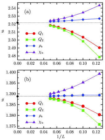
Figure 6: (Color online) Convergence vs the inverse lattice size of intersection points of curves for $L$ and $2L$, for the full (a) and incomplete (b) bilayers. The error bars are are much smaller than the symbols. The circles at $1/L=0$ indicate the critical couplings from the careful finite-size scaling analysis carried out in Sec. III B.

For both models, especially the incomplete bilayer, the spin stiffness crossing point exhibits the most rapid convergence (i.e., the weakest subleading corrections). It and the susceptibility converge from above, while the Binder ratios converge from below. We can hence bracket $g_{\text{c}}$ using these results. However, a much more precise bracketing can be obtained from the spin stiffness curves alone, noting that they become very flat as $L$ grows. With the curvature decreasing with increasing $L$, a straight-line extrapolation using a few large-$L$ points (we use four) should give a lower bound for $g_{\text{c}}$, while the crossing point for the largest $L$ should be an upper bound. The critical couplings extracted this way are $g_{\text{c}}\in(2.5205,2.5232)$ and $g_{\text{c}}\in(1.38870,1.38895)$ for the full and incomplete bilayers, respectively. These values are fully consistent with the best previous estimates, discussed in Sec. I, but the precision is significantly higher. The more rigorous data analysis discussed below will further improve on the accuracy.

Naively, one might expect that the asymptotic approach of the crossing points to the critical coupling should be given by the correlation-length exponent $\nu$, as $g_{\rm cross}=g_{\text{c}}+aL^{-1/\nu}$, as is the case for fixed-size estimates of the critical coupling (or the critical temperature), such as the location of the maximum of the order-parameter susceptibility or the specific heat (in the case of finite-$T$ transitions). However, a crossing point cannot be regarded as a conventional fixed-$L$ definition of $g_{\text{c}}$, since two system sizes are involved and there can be cancelations of a leading behavior defined in terms of the individual lattices. Thus, we would in general expect the crossing points to converge faster than $L^{-1/\nu}$. Binder has discussed the corrections to the cumulant crossing-points,BinderPRL1981 and in a recent article KevinPRE05 we have presented a different way of analyzing crossing points in general (i.e., not only for Binder ratios but also for other quantities that are size-independent at $g_{\text{c}}$) which takes subleading finite-size corrections into account explicitly. There we also showed some results for the spin stiffness crossings of the full bilayer model. Here we will not analyze the crossing points in any greater detail, but instead consider the scaling of the full fixed-$L$ curves shown in the figures of Sec. II. Such “data collapse” makes better use of the full range of simulation results and can also be carried out with subleading corrections taken into account.KevinPRE05

III.2 Finite-Size Scaling with Subleading Corrections

The scaling ansatz typically used to analyze finite-size data $A(t,L)$ for a quantity $A$ at reduced coupling $t=(g-g_{\text{c}})/g_{\text{c}}$ on a lattice of length $L$ is

$$A(t,L)=L^{\kappa/\nu}f_{A}(tL^{1/\nu}),$$ (19)

where $\kappa$ is a critical exponent which depends on the quantity $A$, i.e., $A(t,L=\infty)\sim t^{-\kappa}$. This form can be used to collapse data in a neighborhood of $t=0$, by graphing $A(t,L)L^{\kappa/\nu}$ versus $tL^{-1/\nu}$, adjusting $g_{\text{c}}$, $\kappa$, and $\nu$ to obtain the tightest collapse of the data onto a single curve.

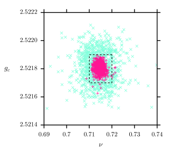
Figure 7: (Color online) The blue crosses $(\times)$ show the input points of the optimization procedure. The red plusses $(+)$ show the output. The dashed black line indicates the magnified region correspondig to the bottom-right plot in Fig. 8.

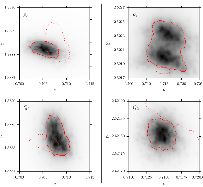
Figure 8: (Color online) The number density of bootstrapped $(\nu,g_{\text{c}})$ solutions is plotted for $Q_{2}$ and $\rho_{\text{s}}$ in greyscale. The left panel shows the incomplete bilayer and the right panel the complete bilayer. The solid red lines show the contour at 1/3 the maximum density (this would correspond to 2/3 of the weight under a gaussian distribution). In the top right panel, note a two-peak structure which sometimes appears in the nonlinear fits. The dotted lines are guides to the eye. They show the $Q_{2}$ contour on the $\rho_{\text{s}}$ plot and vice versa.

In Ref. KevinPRE05, we started from renormalization group theory and derived an extension to (19) that includes both “shift” and “renormalization” corrections:

$$A(t,L)=L^{\kappa/\nu}(1+cL^{-\omega})g_{A}(tL^{1/\nu}+dL^{-\phi/\nu}).$$ (20)

Here, $\phi$ is the subleading irrelevant RG eigenvalue, which causes a shift in the critical coupling. $\omega$ is an effective exponent that accounts for corrections due to the inhomogeneous part of the free energy and nonlinearity of the scaling fields. The constants $c$ and $d$ are nonuniversal and should be regarded as fitting parameters along with the leading and subleading exponents. From Eq. (20), we see that we can now achieve data collapse by plotting $A(t,L)L^{-\kappa/\nu}/(1+cL^{-\omega})$ versus $x=tL^{1/\nu}+dL^{-\phi/\nu}$ for different sizes $L$.

To carry out this type of analysis in practice, we note that the scaling function $g_{A}(x)$ is well-behaved and can be Taylor expanded close to the critical point:

$$g_{A}(x) = A(t,L)L^{-\kappa/\nu}/(1+cL^{-\omega})$$

$$= q_{0}+q_{1}x+q_{2}x^{2}+q_{3}x^{3}+q_{4}x^{4}+\cdots$$

For the Heisenberg bilayers, the critical indices $\kappa$ and $\nu$ are expected to be those of the 3D classical Heisenberg universality class. In the case of the ratios we are considering, $\kappa/\nu=$ are known integers which we hence do not have to adjust. The current best estimate for the correlation length exponent is $\nu=0.7112(5)$,CompostriniPRB2002 but in our analysis we keep it as a free parameter, along with $g_{\text{c}}$, the subleading exponents $\omega$ and $\phi$, the constants $c$ and $d$, and the parameters of the polynomial in (III.2). This amounts to a large number of fitting parameters, but it should be noted that the polynomial expansion of the scaling function is essentially just an interpolation of the data and hence is highly constrained; the freedom in the coefficients $q_{i}$ do not add significant freedom to the other paramers of the fit (we use a quartic polynomial). Moreover, the number of fitting parameters is dwarfed by the number of data points to be fit (hundreds or thousands).

Nonlinear curve fitting has well-known problems associated with the convergence of the parameters to the globally optimal fit. In our work we already know rather accurate estimates for $\nu$ and $g_{\text{c}}$, and at the first stage of the fits we used those values as initial conditions. Once we obtained rough estimates for $c,\omega,d,\phi$, we used the following procedure: Performing bootstrap sampling of the raw data, we carried out a large number (typically around 1000) of fits with initial conditions for all the parameters taken at random from inside a “box” in parameter space. This box is determined such that the fits converge well, but that the variation in starting points is significantly larger than the final spread of the resulting parameters. We then use the spread among the bootstrap samples to calculate statistical errors. This procedure is illustrated in Figs. 7 and 8.

The scaling formula, Eq. (20), is strictly valid only for a small range of couplings in the vicinity of $g_{\text{c}}$ [although the range of validity should be larger than with the leading-order form (19)]. The parameters obtained show some dependence on the range of data included. In order to eliminate as much as possible potential remaining effects of further subleading corrections that are not captured by our approach, we chose to use a rather narrow window in the scaled coupling $x=(g-g_{\text{c}})L^{1/\nu}/g_{\text{c}}+dL^{-\phi/\nu}$, so that there is no longer any statistically detectable dependence on the size of the window. Our final results are based on $x\in[-0.25,0.25]$. There are also other subtle issues in the fitting procedure, e.g., for a given range of $x$, different number of data points are available for the different lattice sizes, typically leading to relatively smaller statistical weight for the larger sizes than the smaller sizes. We therefore made sure to include only system sizes sufficiently large for the extracted parameters not to change appreciably when systematically excluding more of the smaller lattices. We kept only $L\geq 8$ for the results we report here.

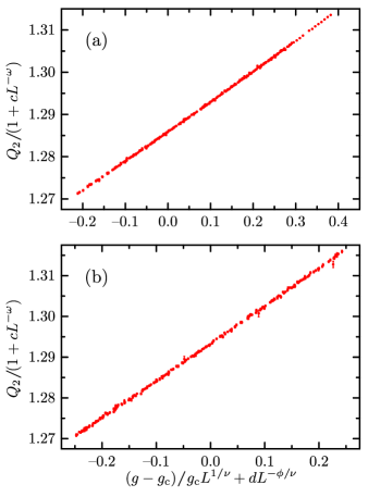
Figure 9: (Color online) Data collapse of the Binder ratio for the full (a) and incomplete (b) bilayer. The values of $g_{\text{c}}$ and $\nu$ obtained are listed in Table 1.

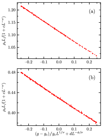
Figure 10: (Color online) Data collapse of the spin stiffness ratio for the full (a) and incomplete (b) bilayer. The values of $g_{\text{c}}$ and $\nu$ obtained are listed in Table 1.

We found both the Binder ratio and the spin stiffness to be well behaved in the fitting procedures. The resulting collapsed data for these quantities, i.e., their scaling functions $g_{A}(x)$ in Eq. (III.2), are shown in Figs. 9 and 10. We do not discuss results for $Q_{1}$ here as it behaves similarly to $Q_{2}$ and is statistically strongly correlated to it. The long-wavelength susceptibility also exhibits data collapse, however with substantially larger fluctuations than $\rho_{\text{s}}$ and $Q_{2}$ (the prefactor $d$ appears to be rather large and difficult to determine accurately, and thus it is difficult to fix the data window $x\in[x_{\rm min},x_{\rm max}]$ in a meaningful way). We have therefore focused on $\rho_{\text{s}}$ and $Q_{2}$ for the final high-precision statistical analysis.

The final parameters and their statistical errors were determined from the bootstrap samples. The distributions are illustrated by density plots in Fig. 8. We list the values for $g_{\text{c}}$, $\nu$, and the value of the respective quantities at the critical point, $q_{c}=Q_{2}(g_{\text{c}}),\rho_{\text{s}}(g_{\text{c}})L$, in Table 1. The critical couplings are here consistent among all the fits, and the correlation length exponent is marginally consistent (within 2–3 standard deviations).

As seen in the table, The highest relative precision of $g_{\text{c}}$ is obtained using $Q_{2}$ for the full bilayer and $\rho_{\text{s}}$ for the incomplete bilayer. The latter can probably be traced to very small subleading corrections, as is evident already in Fig. 4. For the full bilayer $\rho_{\text{s}}$ also has smaller subleading corrections than $Q_{2}$, but still we obtain a higher accuracy in $g_{\text{c}}$ using $Q_{2}$. This shows that small subleading corrections are not necessarily advantageous; what matters is how well those corrections are described by the finite-size scaling forms used. This in turn should be determined by the extent of corrections of even higher order.

For the subleading exponents $\omega$ and $\phi$ we obtain values around unity, except in the case of the $\rho_{\text{s}}$ scaling of the incomplete bilayer, which requires larger values. For the full bilayer, $\omega=1.14(3)$, $\phi=0.8(2)$ in the $Q_{2}$ scaling and $\omega=1.0(3)$, $\phi=1.2(2)$ in the $\rho_{\text{s}}$ scaling. For the incomplete bilayer, $\omega=1.0(4)$, $\phi=1.3(2)$ in $Q_{2}$ and $\omega=1.9(2)$, $\phi=1.8(2)$ in $\rho_{\text{s}}$. All these subleading exponents should be interpreted as effective ones, as they are to some extent affected by the higher-order corrections that we have neglected. The fact that $\omega$ and $\phi$ obtained from $\rho_{\text{s}}$ of the incomplete bilayer are close to $2$ suggests that in this case the leading corrections are small and the exponents instead reflect predominantly the corrections of the next higher order.

Table 1: Bootstrap averages and errorbars for the parameters $g_{\text{c}},\nu,q_{0}$ (the values of the respective quantities at $g_{\text{c}}$). The top group of values are for the incomplete bilayer, and the bottom group for complete bilayer. The indicated error bars correspond to one standard deviation of the probability distributions obtained in the bootstrap analysis, as explained in the text.

	$g_{\text{c}}$	$\nu$	$q_{0}$
$Q_{2}$	1.38885(5)	0.708(2)	1.293(3)
$\rho_{\text{s}}L$	1.38882(2)	0.705(2)	0.434(3)
$\chi_{u}L$	1.388(1)	0.7(1)	0.28(2)
$Q_{2}$	2.52180(3)	0.715(2)	1.2858(3)
$\rho_{\text{s}}L$	2.5221(2)	0.714(5)	1.13(3)
$\chi_{u}L$	2.521(1)	0.7(1)	0.12(2)

IV Summary and Conclusions

We have carried out finite-size scaling analyses of high-precision stochastic series expansion QMC data for two $S=1/2$ Heisenberg bilayer models. Using three different quantities, the Binder order parameter moment ratio, the spin stiffness, and the long-wavelength magnetic susceptibility, we obtained very accurate estimates for the critical couplings. We have stressed the importance of including subleading corrections in the finite-size scaling analysis. All the quantities considered then give mutually consistent results for the critical couplings as well as for the correlation-length exponent $\nu$. We have assumed that the dynamic exponent $z=1$, and all our results are completely consistent with this expectation.ChakravartyPRL1988

The inclusion of two different subleading corrections in the data fits implies larger statistical fluctuations compared to an analysis neglecting subleading corrections or taking them into account less completely than we have done here. However, because of these procedures, along with careful studies of the dependence on the range of system sizes and the data window around the critical point, we are confident that the remaining errors are purely statistical and accurately captured by the error bars quoted in Table 1. We also note that the different quantities we have considered correspond to averaging functions of very different properties of the configurations generated in the simulations—the staggered magnetization in the case of the Binder ratio, the winding number in the case of the spin stiffness, and the long-wavelength magnetization in the case of the susceptibility. The consistency among all the results obtained also contribute to our confidence in the procedures.

Our final estimates for the critical couplings, taking statistically weighted averages of the values listed in Table 1, are $g_{\text{c}}=2.52181(3)$ and $1.38882(2)$ for the full and incomplete bilayer, respectively. Thus we have improved the precision by two orders of magnitude relative to previous calculations. Knowledge of the critical couplings to this level of accuracy should be useful for studies of various aspects of quantum criticality at low temperature in these systems, as one can avoid, to a higher degree than previously, effects from the eventual cross-over to renormalixed classical or quantum-disordered behavior as deviations from $g_{\text{c}}$ become relevant as $T\to 0$.

For the correlation length, a weighted average of the four results from $\rho_{\text{s}}$ and $Q_{2}$ listed in Table 1 gives $\nu=0.7106(9)$. This is consistent within error bars with the currently most accurate estimate of the 3D classical Heisenberg exponent, $\nu=0.7112(5)$, obtained from classical 3D Heisenberg simulations in Ref. CompostriniPRB2002, .

Taking a statistical average of the four individual results for $\nu$ (and analogously for $g_{\text{c}}$ discussed above) is motivated here in spite of the fact that they are obtained in only two different simulations. This is because the winding numbers (giving $\rho_{\text{s}}$) and the sublattice magnetization (giving $Q_{2}$) are very weakly correlated in the simulations. We regard it as pure coincidence that the two values for each model in Table 1 are closer to each other than those of different models, and not an indication of a potentially different universality class in the incomplete bilayer (due to incomplete cancelation of Berry phases HaldanePRL1988 ; ChakravartyPRL1988 ; ChubukovPRB1994 ; TroyerJPJ1997 ) when the layer-exchange symmetry is not present. The very close agreement of the universal Binder ratio at $g_{\text{c}}$ also speaks in favor of the same universality class for both lattices.

Although we have not quite reached the accuracy for $\nu$ obtained in the most recent classical simulations CompostriniPRB2002 (although our final error bar is actually only approximately twice as large), the precision is still sufficiently high to further increase the confidence in the belief that the universality class of the transition is that of the 3D classical Heisenberg model. The previously best (to our knowledge) determination of $\nu$ for the transition in a 2D Heisenberg system is $0.70(1)$.MatsumotoPRB2001

We do not find the predicted WallinPRB1994 universality of $\rho_{\text{s}}L$ at the critical point (whereas we do find the expected universality in the case of the Binder ratio); the values for the full and incomplete bilayer differ by about $30\%$. On the other hand, in recent simulations of the finite-$T$ transition of the 3D $S=1/2$ Heisenberg ferromagnet and antiferromagnet,heis3d we find consistent values for both models at $T_{\text{c}}$. Thus we are lead to speculate that there is some geometrical effect affecting the stiffness, so that universality might hold for different critical points (arrangement of couplings allowing a transition) on the same lattice but not necessarily for lattices with different unit cells.

This work was supported by the NSF under grant No. DMR-0513930.

References

- (1) E Manousakis, Rev. Mod. Phys. 63, 1 (1991).
- (2) H. M. Rønnow et al., Phys. Rev. Lett. 87, 037202 (2001).
- (3) S. Chakravarty, B. I. Halperin, and D. R. Nelson, Phys. Rev. Lett. 60, 1057 (1988).
- (4) J.-K. Kim and M. Troyer, Phys. Rev. Lett. 80, 2705 91998).
- (5) A. W. Sandvik and D. J. Scalapino, Phys. Rev. B 51, 9403 (1995).
- (6) F. D. M. Haldane, Phys. Rev. Lett. 50, 1153 (1983).
- (7) S. Sachdev, Quantum Phase Transitions (Cambridge University Press, Cambridge 1999).
- (8) F. D. M. Haldane, Phys. Rev. Lett. 61, 1029 (1988).
- (9) J. D. Reger and A. P. Young, Phys. Rev. B 37, 5493 (1988).
- (10) A. V. Chubukov, S. Sachdev, and J. Ye, Phys. Rev. B 49, 11919 (1994).
- (11) K. Hida, J. Phys. Soc. Jpn., 59, 2230 (1990); ibid. 61 , 1013 (1992).
- (12) A. J. Millis and H. Monien, Phys. Rev. Lett. 70, 2810 (1993).
- (13) A. W. Sandvik and D. J. Scalapino, Phys. Rev. Lett. 72, 2777 (1994)
- (14) R. R. P. Singh and M. P. Gelfand, Phys. Rev. Lett. 61, 2484 (1988).
- (15) M. Troyer, H. Kontani, and K. Ueda, Phys. Rev. Lett. 76, 3822 (1996).
- (16) P. V. Shevchenko, A. W. Sandvik, O. P. Sushkov, Phys. Rev. B 61, 3475 (2000).
- (17) W. Brenig, cond-mat/0502489.
- (18) C. Holm and W. Janke, Phys. Rev. B 48, 936 (1993).
- (19) M. Campostrini, M. Hasenbusch, A. Pelissetto, P. Rossi, and E. Vicari, Phys. Rev. B 65, 144520 (2002).
- (20) V. N. Kotov, O. Sushkov, Z. Weihong, and J. Oitmaa, Phys. Rev. Lett. 80, 5790 (1998)
- (21) S. Sachdev, C. Buragohain, and M. Vojta, Science 286, 2479 (1999).
- (22) M. Troyer, Prog. Theor. Phys. Suppl. 145, 326 (2002).
- (23) S. Sachdev and M. Vojta, Phys. Rev. B 68, 064419 (2003).
- (24) O. Sushkov, Phys. Rev. B 68, 094426 (2003).
- (25) K. H. Höglund and A. W. Sandvik (unpublished).
- (26) K. S. D. Beach, L. Wang, and A. W. Sandvik, cond-mat/0505194.
- (27) A. W. Sandvik, Phys. Rev. B 59, R14157 (1999).
- (28) A. A. Caparica, A. Bunker, and D. P. Landau, Phys. Rev. B 62, 9458 (2000).
- (29) M. Wallin, E. S. Sørensen, S. M. Girvin, and A. P. Young, Phys. Rev. B 49, 12115 (1994).
- (30) M. P. A. Fisher, P. B. Weichman, G. Grinstein, and D. S. Fisher, Phys. Rev. B 40, 546 (1989).
- (31) K. Binder, Phys. Rev. Lett. 47, 693 (1981); Z. Phys. B 43, 119 (1981).
- (32) A. W. Sandvik, Phys. Rev. B 56, 11678 (1997).
- (33) E. L. Pollock and D. M. Ceperley, Phys. Rev. B 36, 8343 (1987).
- (34) N. Elstner and R. R. P. Singh, Phys. Rev. B 57, 7740 (1998).
- (35) M. Troyer, M. .E. Zhitomirsky, and K. Ueda, Phys. Rev. B 55, R6117 (1997).
- (36) M. Troyer, M. Imada, and K. Ueda, J. Phys. Soc. Jpn. 66, 2957 (1997).
- (37) M. Matsumoto, C. Yasuda, S. Todo, and H. Takayama, Phys. Rev. B 65, 014407 (2001).
- (38) K. S. D. Beach and A. W. Sandvik (work in progress).