On-Chip Microwave Fock States and Quantum Homodyne Measurements

Abstract

We propose a method to couple metastable flux-based qubits to superconductive resonators based on a quantum-optical Raman excitation scheme that allows for the deterministic generation of stationary and propagating microwave Fock states and other weak quantum fields. Moreover, we introduce a suitable microwave quantum homodyne technique, with no optical counterpart, that enables the measurement of relevant field observables, even in the presence of noisy amplification devices.

A two-level atom coupled to a single mode of a quantized electromagnetic field is arguably the most fundamental system to exhibit matter-radiation interplay. Their interaction, described by the Jaynes-Cummings (JC) model, arises naturally in the realm of cavity quantum electrodynamics (CQED) in the microwave Raimond:2001:a and optical domains Mabuchi:2002:a . There, a variety of nonclassical states (e.g., squeezed, Schrödinger cat, and Fock states) and other remarkable phenomena and applications (e.g., entanglement and elements of quantum logic Nielsen:2000:a ) have been proposed and realized. Other physical systems, like trapped ions Leibfried:2003:a , can reproduce the JC dynamics and, consequently, exploit this analogy for similar purposes. The intracavity field in CQED and the motional field of the trapped ions are typically detected through a suitable transfer of information to measurable atomic degrees of freedom Raimond:2001:a ; Leibfried:2003:a . In the case of propagating fields, quantum homodyne detection Leonhardt:1997:a , a method based on efficient photodetectors, leads to quantum state tomography Lvovsky:2001:a .

Given its relevance for quantum communication, single-photon sources have been pursued in the optical domain Kuhn:2002:a ; Keller:2004:a . Recently, several CQED-related experiments have been performed in tunable, solid-state systems. Quantum dots in photonic band-gap structures have been used as single photon sources Badolato:2005:a and superconducting qubits have been coupled to on-chip cavities Wallraff:2004:a ; Chiorescu:2004:a . In addition, microwave squeezing with Josephson parametric amplifiers Movshovich:1990:a and aspects of the quantum-statistical nature of GHz photons in mesoscopic conductors have been demonstrated Gabelli:2004:a .

In this Letter, we propose the implementation of a deterministic source of microwave Fock states, or linear superpositions of them, at the output of a superconducting resonator containing a flux qubit. A Raman-like scheme Francsa:Santos:2001:a determines the coupling between the cavity and the qubit that consists of two metastable states of a three-level system in a $\Lambda$-type configuration Yang:2004:a ; Murali:2004:a ; Liu:2004:a ; Siewert:2005:a . Furthermore, we show that relevant observables of these weak quantum signals can be characterized by a microwave quantum homodyne measurement (MQHM) scheme. This is a specially engineered technique based on a hybrid ring junction Collin:2000:a ; Sarovar:2005:a acting as an on-chip microwave beam splitter (MBS). Given that direct microwave photodetectors are not yet available, the measurement device consists of linear phase-insensitive amplifiers followed by square-law detectors (and/or mixers) and an oscilloscope (or spectrum analyzer). These fundamental tools represent building blocks to establish on-chip quantum information transfer between qubits.

A prototypical example of a flux-based quantum circuit is the radio-frequency (RF) superconducting quantum-interference device (SQUID), a superconducting loop interrupted by a single Josephson tunnel junction. The RF SQUID Hamiltonian is

$$\hat{H}_{\rm S}\ =\ \frac{\hat{Q}^{2}}{2C_{\rm j}}+\frac{(\hat{\Phi}-\Phi_{\rm x})^{2}}{2L_{\rm s}}-E_{\rm J}\cos\bigg{(}2\pi\frac{\hat{\Phi}}{\Phi_{0}}\bigg{)},$$ (1)

where $\hat{Q}$ is the charge stored on the junction capacitor $C_{\rm j}$, $\hat{\Phi}$ is the total flux threading the loop (with $[\hat{\Phi},\hat{Q}]=i\hbar$), $\Phi_{\rm x}$ is an externally applied quasi-static flux bias, $L_{\rm s}$ is the self-inductance of the loop, $E_{\rm J}\equiv I_{{\rm c}0}\Phi_{0}/2\pi$ is the Josephson coupling energy, $I_{{\rm c}0}$ is the junction critical current, and $\Phi_{0}=h/2e$ is the flux quantum.

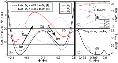
Figure 1: (Color online) (a) Potential profile of the RF SQUID for two distinct values of $\Phi_{\rm x}$ [(I) and (II)] and wave functions for the first three lowest energy levels ($|{\rm g}\rangle$, $|{\rm e}\rangle$, and $|{\rm h}\rangle$). Parameters are given in Table I. The Raman scheme is indicated with arrows. (b) RF SQUID energy-band diagram near $\Phi_{0}/2$ plotted vs. $\Phi_{\rm x}$. Zero detuning case, point (I), and large detuning case, point (II). (c) Absolute value of the vacuum Rabi frequency $g_{\rm he}$ as a function of $\Phi_{\rm x}$. The coupling reaches 56 MHz at the anticrossing between levels $|{\rm e}\rangle$ and $|{\rm h}\rangle$.

For appropriate design parameters, and close to half-integer values of $\Phi_{\rm x}/\Phi_{0}$, the RF SQUID potential profile becomes a relatively shallow double well whose asymmetry can be tuned by setting $\Phi_{\rm x}$ (see Fig. 1). In this case, the two lowest eigenstates $|{\rm g}\rangle$ and $|{\rm e}\rangle$ are metastable and localized in the left and right wells respectively, whereas the excited state $|{\rm h}\rangle$ is delocalized with energy above the barrier. As will be shown later, these levels are suitable for implementing a Raman excitation scheme. The energy levels can be tuned by statically biasing $\Phi_{\rm x}$ during the experiment and transitions between states are driven by pulsed AC excitations. Because of their relatively large excited-state lifetimes, persistent-current (PC) qubits Chiorescu:2004:a can also be considered for the purposes of this work.

The segment of superconducting coplanar waveguide (CWG) shown in Figs. 2 (a), (b), and (d) is one realization of an open-circuited transmission line resonator capacitively coupled to a CWG transmission line. Such a cavity is characterized by eigenenergies with transition angular frequencies $\omega_{k}=2\pi f_{k}$ that are much larger than the thermal energy at cryogenic temperatures. Its Hamiltonian is $\hat{H}_{\rm C}=\sum_{k}\hbar\omega_{k}\Big{(}\hat{a}^{\dagger}_{k}\hat{a}_{k}+1/2\Big{)}$, where $\hat{a}^{\dagger}_{k}$ and $\hat{a}_{k}$ are the bosonic creation and annihilation operators for mode $k$. Current and voltage, corresponding to magnetic and electric fields respectively, are conjugate operators associated with the quantized resonator, $\hat{I}_{\rm c}(z,t)=(\partial/\partial t)\,\hat{\vartheta}(z,t)$, where $z$ is the spatial coordinate for the superconducting inner strip and $\hat{\vartheta}(z,t)$ is the normal mode expansion of the cavity field Blais:2004:a . The vacuum current for the odd, $k_{\rm o}$, and even, $k_{\rm e}$, cavity modes is $I^{0}_{{\rm c},k_{\rm o/e}}(z)=\sum_{k_{\rm o}=1}^{\tilde{k}_{\rm o}}\sqrt{\hbar\omega_{k_{\rm o}}/(Dl)}\cos\big{(}k_{\rm o}\pi z/D\big{)}+\sum_{k_{\rm e}=2}^{\tilde{k}_{\rm e}}\sqrt{\hbar\omega_{k_{\rm e}}/(Dl)}\sin\big{(}k_{\rm e}\pi z/D\big{)}$, where $\tilde{k}_{\rm o}$, $\tilde{k}_{\rm e}$ are upper cutoffs for the odd and even modes respectively Blais:2004:a , $D=\lambda/2$ is the length of the resonator ($\lambda$ is the full wavelength corresponding to $\omega_{k_{\rm o}=1}$), and $l$ is its total series inductance per unit length. Hereafter, the cavity is chosen to be operated at $k_{\rm 0}=1$ and is assumed to have an external quality factor $Q_{\rm x}\sim 10^{4}$ at $f_{1}=\omega_{1}/2\pi\sim 10$ GHz, corresponding to a cavity decay rate $\kappa_{\rm c}\sim 1$ MHz Wallraff:2004:a . Hence, at a base temperature $T_{\rm b}\sim 50$ mK, the mean number of thermal photons is $\langle n_{\rm th}\rangle=[\exp(\hbar\omega_{1}/k_{\rm B}T_{\rm b})-1]^{-1}\approx~{}10^{-4}$ and the cavity mode can be considered to be in the vacuum state $|0\rangle$.

Embedding the RF SQUID in the CWG cavity allows an inductive coupling between any two levels of the RF SQUID and a single cavity mode $k$. The resulting interaction Hamiltonian is $\hat{H}_{\rm I}=-M_{\rm cs}\hat{I}_{{\rm c},k}\hat{I}_{\rm s}$, where $\hat{I}_{{\rm c},k}$ and $\hat{I}_{\rm s}$ are the resonator and the RF SQUID current operators respectively and $M_{\rm cs}$ is their mutual inductance. Using the explicit forms of the current operators, we find

$$\hat{H}_{\rm I}\,=\,-\ (M_{\rm cs}/L_{\rm s})\,I^{0}_{{\rm c},k}(z)\ (\hat{\Phi}-\Phi_{\rm x})\ i\,[\hat{a}^{\dagger}_{k}(t)-\hat{a}_{k}(t)].$$ (2)

The RF SQUID can be positioned near one of the antinodes of the vacuum current [e.g., see Figs. 2 (a) and (b) for $k_{\rm o}=1$] and can be biased to yield maximum coupling for any two of its eigenstates $|i\rangle$ and $|j\rangle$. The interaction matrix element between these levels represents their coupling strength with mode $k$ and it is used to define the vacuum Rabi frequency $g_{ij}=-\,(M_{\rm cs}/L_{\rm s})I^{0}_{{\rm c},k}(z)\langle i|\hat{\Phi}|j\rangle/h$. Moreover, when operating the system in the dispersive regime, the corresponding RF SQUID decay rates $\gamma_{ij}$ become $\gamma^{\rm eff}_{ij}=\gamma_{ij}(g_{ij}/\delta_{ij})^{2}$, where $\delta_{ij}$ is the detuning between mode $k$ and the transition under consideration. The coupling $g_{\rm he}$, the effective decay rate $\gamma^{\rm eff}_{\rm he}$, and other relevant quantities have been calculated for both RF SQUIDs and PC qubits and typical results are reported in Table I.

A main application of the system illustrated above is the generation of single photons at frequency $f_{k}$ in a manner similar to a quantum-optical Raman scheme Francsa:Santos:2001:a ; Keller:2004:a . After preparing the RF SQUID in level $|{\rm g}\rangle$, the transition $|{\rm g}\rangle\leftrightarrow|{\rm h}\rangle$ is driven by a classical excitation with Rabi frequency $\Omega_{\rm gh}\sim g_{\rm he}$ and detuned by the amount $\delta$. The same transition is detuned from the resonator mode $k$ by an amount $\Delta\gg\delta$, resulting in a comparatively negligible coupling. On the other hand, the $|{\rm h}\rangle\leftrightarrow|{\rm e}\rangle$ transition is the only one coupled to mode $k$ and it is also detuned by $\delta$ [see Figs. 1 (a) and (b)]. Choosing $\delta\gg\max\left[\Omega_{\rm gh},g_{\rm he}\right]$, level $|{\rm h}\rangle$ can be adiabatically eliminated Francsa:Santos:2001:a ; Keller:2004:a , thus leading to the effective second-order Hamiltonian

$$\hat{H}_{{\rm eff}} = \hbar\frac{\Omega_{{\rm gh}}^{2}}{\delta}|{\rm g}\rangle\langle{\rm g}|+\hbar\frac{g_{{\rm he}}^{2}}{\delta}|{\rm e}\rangle\langle{\rm e}|\hat{a}^{\dagger}_{k}\hat{a}_{k}+{}$$ (3)

$$+\ \hbar g_{{\rm eff}}\left(|{\rm g}\rangle\langle{\rm e}|\hat{a}_{k}+|{\rm e}\rangle\langle{\rm g}|\hat{a}^{\dagger}_{k}\right),$$

where $g_{\rm eff}=(\Omega_{\rm gh}/\delta)g_{\rm he}$ is the effective Raman coupling. The first two terms at the r.h.s. of Eq. (3) are AC Zeeman shifts, while the last term describes an effective anti-JC dynamics, inducing transitions within the $\{|{\rm g}\rangle|n\rangle,|{\rm e}\rangle|n+1\rangle\}$ subspaces. The AC Zeeman shifts associated with the transition of interest $\{|{\rm g}\rangle|0\rangle,|{\rm e}\rangle|1\rangle\}$, can be compensated by retuning the classical driving frequency. When the strong-coupling regime is reached, $g_{\rm eff}\gtrsim\max\left[\kappa_{\rm c},\gamma^{\rm eff}_{\rm he}\right]$, an effective $\pi$-pulse realizes a complete transfer of population from state $|{\rm g}\rangle|0\rangle$ to state $|{\rm e}\rangle|1\rangle$. This process leads to the creation of a microwave Fock state $|1\rangle$ inside the resonator that will leak out in a time $\sim 1/\kappa_{\rm c}$. In the case of weak-coupling, the photon leaks to the outer world as soon as it is generated inside the cavity, thereby realizing a deterministic single-photon source. Tailoring the photon pulse shape would require a time-dependent classical driving $\Omega_{\rm gh}(t)$ Keller:2004:a .

If the initial qubit-cavity state is $(\cos\theta|{\rm g}\rangle+e^{i\phi}\sin\theta|{\rm e}\rangle)|0\rangle$, then the above Raman $\pi$-pulse would map it onto the cavity field ($|{\rm e}\rangle|0\rangle$ is a dark state of the anti-JC dynamics). In this way, we would be able to produce an outgoing field state $\cos\theta|1\rangle+e^{i\phi}\sin\theta|0\rangle$.

The proposed Raman scheme allows for generating single photons without initialization of the qubit in the excited state $|{\rm e}\rangle$ ($|{\rm g}\rangle|0\rangle$ is not a dark state of the anti-JC dynamics). Raman pulses are fast compare to STIRAP (adiabatic) techniques Kuhn:2002:a and exploit the well defined qubit-cavity coupling Keller:2004:a , intrinsic in our scheme.

Table 1: Typical parameters and relevant quantities for RF SQUIDs and PC qubits, coupled to a 50 $\Omega$ resonator Resonator:extra:parameters .

	$I_{{\rm c}0}$	$C_{\rm j}$	$L_{\rm s}$	$M_{\rm cs}$	$\frac{\Delta E_{\rm he}}{h}$	$I^{0}_{{\rm c},1}$	$|g_{\rm he}|$	$\gamma^{\rm eff}_{\rm he}$
	($\mu$A)	(fF)	(pH)	(pH)	(GHz)	(nA)	(MHz)	(kHz)
RF SQUID	1.4	100	266	22.2	6.2	32	28	2.5
PC qubit	0.64	7	17	1.4	5.8	31.5	30	2.5

Measurement schemes based on classical homodyning Collin:2000:a are insufficient to resolve nonclassical field states. On the other hand, microwave single-photon detectors in mesoscopic systems do not exist to our knowledge. Here, we propose an MQHM technique as a means to measure relevant observables of weak quantum signals, even at the level of single photons. This can be implemented in three main steps. First, a signal (S) and a local oscillator (LO), characterized by the same angular frequency $\omega_{\rm S}=\omega_{\rm LO}$, are coherently superposed at a suitably designed MBS cooled to base temperature [Fig. 2 (a)]. Second, the microwave fields at the MBS output ports are amplified at low temperatures by means of linear phase-insensitive amplifiers. Third, the amplified signals are then downconverted to DC currents $I_{{\rm s},2/4}$, proportional to the energies of the input signals, via square-law detectors (and/or mixers) at room temperature Collin:2000:a . The DC currents can be measured as voltages with an oscilloscope. Adequate manipulation of these measurements will lead to signal information with minimal noise background.

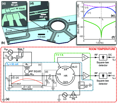
Figure 2: (Color online) (a) Sketch of the entire generation and measurement network ($C_{\rm in}$, $C_{1}$, and $C_{2}$: capacitive $\Pi$ network representing the resonator input port acting as a mirror; $C_{\rm p}$: parasitic capacitor at the cavity open-circuit ending; HR: hybrid ring; PS: phase shifter; AT: attenuator). (b) Asymmetric CWG resonator with integrated HR. (c) On-chip antenna providing the classical driving $\Omega_{\rm gh}$. (d) Resonator-CWG coupling region. (e) The waves traveling around the HR interfere resulting in the plotted reflection and transmission amplitude patterns. (f) Isolation between ports three and one of the HR.

The MBS is realized using a suitable four-port device: the hybrid ring [see Figs. 2 (a) and (b)]. The advantageous coplanar design proposed here can easily be scaled and preferably fabricated with low resistivity conductors. We now extend the classical theory of hybrid rings in Ref. Collin:2000:a to the quantum regime by analogy with an optical beam splitter. With only the vacuum incident at ports two and four, and up to a global phase common to both input beams, the reduced quantum input-output relations of a lossless MBS are

$$\left[\begin{array}[]{c}\hat{a}_{2}\\ \hat{a}_{4}\end{array}\right]\ =\ \left[\begin{array}[]{cc}r&t\\ -t^{*}&r^{*}\end{array}\right]\ \left[\begin{array}[]{c}\hat{a}_{\rm S}\\ \hat{a}_{\rm LO}\end{array}\right].$$ (10)

Here, $r$ and $t$ are the complex, frequency-dependent reflection and transmission coefficients, $\hat{a}_{\rm S}$ and $\hat{a}_{\rm LO}$ are the signal and LO port operators respectively. The latter is chosen to be a classical coherent field that is characterized by its complex amplitude $\alpha_{\rm LO}=|\alpha_{\rm LO}|\exp(i\theta_{\rm r})$, where $|\alpha_{\rm LO}|$ is the norm of the field amplitude and $\theta_{\rm r}$ is its relative phase with respect to S. The numerical simulations plotted in Fig. 2 (e) show that the MBS can be balanced over a broad bandwidth around the desired operation frequency $f_{k}$, i.e., $r=t=1/\sqrt{2}$ ($-$3 dB), with outputs $\hat{a}_{2}=(\hat{a}_{\rm S}+\hat{a}_{\rm LO})/\sqrt{2}$ and $\hat{a}_{4}=(-\hat{a}_{\rm S}+\hat{a}_{\rm LO})/\sqrt{2}$.

At this point, standard optical quantum homodyning would require the use of photodetectors at each output port of the MBS. This would allow different measurements of photocurrents $I_{{\rm p},2/4}$, proportional to different realizations $N$ of the observable $\hat{n}=\hat{a}^{\dagger}\hat{a}$. By computing the difference $I_{{\rm p},2}-I_{{\rm p},4}\propto N_{2}-N_{4}=2|\alpha_{\rm LO}|X_{\theta_{\rm r}}$, where the LO operators were replaced by their complex amplitudes, realizations of the quadrature $\hat{X}_{\theta_{\rm r}}\equiv(\hat{a}^{\dagger}_{\rm S}e^{i\theta_{\rm r}}+\hat{a}_{\rm S}e^{-i\theta_{\rm r}})/2$, enhanced by a factor $2|\alpha_{\rm LO}|$, could be obtained. With the complete histogram of these measurements, all moment averages $\langle\hat{X}^{p}_{\theta_{\rm r}}\rangle$, $\forall p\in\mathbb{N}$, and full reconstruction of the associated Wigner function via quantum tomography might be evaluated Leonhardt:1997:a . In absence of microwave photodetectors, the MBS output signals must go through linear amplifiers, square-law detectors and/or mixers before being measured at the oscilloscope. These conditions impose severe restrictions in the measurement process with no counterpart in the optical regime and require additional theoretical considerations.

The output signals, referred to the input, of linear phase-insensitive amplifiers can be written as ${\hat{X}}_{{\tilde{a}}_{2}}={\hat{X}}_{a_{2}}+{\hat{X}}_{\xi_{2}}$ and ${\hat{X}}_{{\tilde{a}}_{4}}={\hat{X}}_{a_{4}}+{\hat{X}}_{\xi_{4}}$, where ${\hat{X}}_{a}\equiv({\hat{a}}+{\hat{a}}^{\dagger})/2$ and ${\hat{X}}_{\xi}\equiv({\hat{\xi}}+{\hat{\xi}}^{\dagger})/2$ Caves:1982:a . The added noises at each arm, $\hat{\xi}_{2/4}$, are random, uncorrelated, and characterized by (almost) the same noise temperature $T_{\rm n}$, leading to a mean photon number $\langle{\hat{n}}_{\xi}\rangle=\langle{\hat{\xi}}^{\dagger}{\hat{\xi}}\rangle=k_{\rm B}T_{\rm n}/\hbar\omega_{k}$. The difference between the measured currents produced by the square-law detectors, $I_{{\rm s},2}-I_{{\rm s},4}$, is proportional to different realizations of the following observable

$$\!\!\!\!\!\!{\hat{\tilde{a}}}^{\dagger}_{2}{\hat{\tilde{a}}}_{2}-{\hat{\tilde{a}}}^{\dagger}_{4}{\hat{\tilde{a}}}_{4}=\!\!\!\!\! {\hat{a}}^{\dagger}_{\rm S}{\hat{a}}_{\rm LO}+{\hat{a}}^{\dagger}_{\rm LO}{\hat{a}}_{\rm S}+{\hat{\xi}}_{2}^{\dagger}{\hat{\xi}}_{2}-{\hat{\xi}}_{4}^{\dagger}{\hat{\xi}}_{4}$$ (11)

$$+\ {\hat{\xi}}_{2}^{\dagger}\frac{({\hat{a}}_{\rm S}+{\hat{a}}_{\rm LO})}{\sqrt{2}}+{\hat{\xi}}_{2}\frac{({\hat{a}}^{\dagger}_{\rm S}+{\hat{a}}^{\dagger}_{\rm LO})}{\sqrt{2}}$$

$$-\ {\hat{\xi}}_{4}^{\dagger}\frac{(-{\hat{a}}_{\rm S}+{\hat{a}}_{\rm LO})}{\sqrt{2}}-{\hat{\xi}}_{4}\frac{(-{\hat{a}}^{\dagger}_{\rm S}+{\hat{a}}^{\dagger}_{\rm LO})}{\sqrt{2}}.$$

Repeating the measurement procedure, we can average

$$\langle{\hat{\tilde{a}}}^{\dagger}_{2}{\hat{\tilde{a}}}_{2}-{\hat{\tilde{a}}}^{\dagger}_{4}{\hat{\tilde{a}}}_{4}\rangle=2|\alpha_{\rm LO}|\langle\hat{X}_{\theta_{\rm r}}\rangle,$$ (12)

given that $\langle{\hat{\xi}_{2}}\rangle=\langle{\hat{\xi}_{4}}\rangle=0$ and the reasonable assumption $\langle{\hat{n}}_{\xi_{2}}\rangle\sim\langle{\hat{n}}_{\xi_{4}}\rangle$. Equation (12) shows that the proposed MQHM allows the measurement of the enhanced mean value of the quadrature $\hat{X}_{\theta_{\rm r}}$ with negligible noise disturbance. This important physical quantity is sensitive to coherence: it is zero for any Fock state $|n\rangle$ and $\cos{\theta_{\rm r}}/2$ for the superposition $(|0\rangle+|1\rangle)/\sqrt{2}$. However, the method illustrated above does not lead to a measurement of $\langle\hat{X}^{2}_{\theta_{\rm r}}\rangle$ since the amplifier noise shadows the information contained in the signal. Instead, we now propose to send both MBS outputs through mixers, using the same calibrated local oscillator, and then evaluate the ensemble average of the measured products

$$\langle{\hat{X}}_{\tilde{a}_{2},{\theta_{\rm r}}}{\hat{X}}_{\tilde{a}_{4},{\theta_{\rm r}}}\rangle=-\frac{1}{2}\langle\hat{X}^{2}_{{\theta_{\rm r}}}\rangle+\frac{1}{2}\langle\hat{X}^{2}_{\rm LO,{\theta_{\rm r}}}\rangle.$$ (13)

Here, we used $\langle{\hat{X}}_{\xi_{2}}{\hat{X}}_{\xi_{4}}\rangle=\langle{\hat{X}}_{\xi_{2}}\rangle\langle{\hat{X}}_{\xi_{4}}\rangle=0$ and assumed $\langle{\hat{X}}^{2}_{\rm LO,{\theta_{\rm r}}}\rangle$ to be known (after performing an adequate network calibration) or removable (e.g., via a modulation technique). Equation (13) shows a remarkably simple way of measuring $\langle\hat{X}^{2}_{{\theta_{\rm r}}}\rangle$ with minimal noise disturbance.

A precise measurement of $\langle\hat{X}_{\theta_{\rm r}}\rangle$ and $\langle\hat{X}^{2}_{\theta_{\rm r}}\rangle$, as shown in Eqs. (12) and (13), requires random and uncorrelated noise, a sufficient number of repetition measurements, and adequate calibration, if the difference of $\langle{\hat{n}}_{\xi}\rangle$ ($\langle{\hat{n}}_{\xi}\rangle\sim 21$ for $T_{\rm n}\sim 10$ K) for the two amplifiers is not sufficiently small. It is known that the knowledge of $\langle\hat{X}_{\theta_{\rm r}}\rangle$ and $\langle\hat{X}^{2}_{\theta_{\rm r}}\rangle$ provides complete information about Gaussian states and a simple criterion for discriminating Fock states. Furthermore, we conjecture here on the possibility of measuring $\langle\hat{X}^{p}_{\theta_{\rm r}}\rangle$, $\forall p\in\mathbb{N}$, $\forall{\theta_{\rm r}}\in[0,2\pi)$ [see PS in Fig. 2 (a)] under the conditions described above, allowing a complete reconstruction of the Wigner function in the microwave domain.

In conclusion, we proposed a new scheme for the deterministic generation of intracavity and propagating microwave Fock states or linear superpositions of them. We showed also how to realize MQHM for measuring first and second-order field quadrature moments. These proposals are essential tools for the implementation of quantum-optical CQED and linear optics in the microwave domain with superconducting devices on a chip.

The authors thank C. M. Caves, S. M. Girvin, and D. C. Glattli for useful discussions. MM and WDO would like to acknowledge K. R. Brown, D. E. Oates, and Y. Nakamura for fruitful discussions and T. P. Orlando and M. Gouker for their support. This work has been partially supported by the DFG through SFB 631. ES acknowledges EU support through the RESQ project.

References

- (1) J.M. Raimond, M. Brune, and S. Haroche, Rev. Mod. Phys. 73, 565 (2001).
- (2) H. Mabuchi and A.C. Doherty, Science 298, 1372 (2002).
- (3) M.A. Nielsen and I.L. Chuang, Quantum Computation and Quantum Information, (Cambridge University Press, Cambridge, 2000).
- (4) D. Leibfried, R. Blatt, C. Monroe, and D. Wineland, Rev. Mod. Phys. 75, 281 (2003).
- (5) U. Leonhardt, Measuring the Quantum State of Light (Cambridge University Press, Cambridge, 1997).
- (6) A.I. Lvovsky et al., Phys. Rev. Lett. 87, 050402 (2001).
- (7) A. Kuhn, M. Hennrich, and G. Rempe, Phys. Rev. Lett. 89, 067901 (2002).
- (8) M. Keller et al., Nature 431, 1075 (2004).
- (9) A. Badolato et al., Science 308, 1158 (2005).
- (10) A. Wallraff et al., Nature 431, 162 (2004).
- (11) I. Chiorescu et al., Nature 431, 159 (2004).
- (12) R. Movshovich et al., Phys. Rev. Lett. 65, 1419 (1990).
- (13) J. Gabelli et al., Phys. Rev. Lett. 93, 056801 (2004).
- (14) M. França Santos, E. Solano, and R.L. de Matos Filho, Phys. Rev. Lett. 87, 093601 (2001).
- (15) C.-P. Yang, S.-I Chu, and S. Han, Phys. Rev. Lett. 92, 117902 (2004).
- (16) K.V.R.M. Murali et al., Phys. Rev. Lett. 93, 087003 (2004).
- (17) Yu-Xi Liu, L.F. Wei, and F. Nori, Europhys. Lett. 67 (6), 941 (2004).
- (18) J. Siewert et al., e-print cond-mat/0509735.
- (19) R.E. Collin, Foundations for Microwave Engineering, 2nd ed. (Wiley-IEEE Press, New Jersey, 2000).
- (20) M. Sarovar, Hsi-S. Goan, T.P. Spiller, and G.J. Milburn, Phys. Rev. A 72, 062327, (2005).
- (21) A. Blais et al., Phys. Rev. A 69, 062320 (2004).
- (22) E.g., conductor width m, slot m, capacitance and inductance per unit length nFm-1 and nHm-1 respectively, and length mm.
- (23) C.M. Caves, Phys. Rev. D 26, 1817 (1982).