The totally asymmetric exclusion process on a ring:
Exact relaxation dynamics and associated model of clustering transition

Abstract

The totally asymmetric simple exclusion process in discrete time is considered on finite rings with fixed number of particles. A translation-invariant version of the backward-ordered sequential update is defined for periodic boundary conditions. We prove that the so defined update leads to a stationary state in which all possible particle configurations have equal probabilities. Using the exact analytical expression for the propagator, we find the generating function for the conditional probabilities, average velocity and diffusion constant at all stages of evolution. An exact and explicit expression for the stationary velocity of TASEP on rings of arbitrary size and particle filling is derived. The evolution of small systems towards a steady state is clearly demonstrated. Considering the generating function as a partition function of a thermodynamic system, we study its zeros in planes of complex fugacities. At long enough times, the patterns of zeroes for rings with increasing size provide evidence for a transition of the associated two-dimensional lattice paths model into a clustered phase at low fugacities.

Keywords: Totally asymmetric exclusion process, ring geometry, discrete-time update, exact time evolution, zeros of partition function, condensation

I Introduction

The totally asymmetric simple exclusion process (TASEP) is, probably, the simplest model in the kinetic theory of many interacting particles Lig ; Spohn . Being one of the few exactly solvable models of non-equilibrium statistical mechanics, the TASEP describes a nontrivial evolution of the system from an initial configuration to a steady state. While the long-time stage of this evolution and the steady state itself have been studied in details Dhar ; Gwa ; DerEvMuk ; JanLeb ; DerMal ; DerLeb ; Derrida , much less is known about the initial short-time stage even for relatively simple small systems.

The exact solution of the master equation obtained by Schütz Schutz gives a complete description of the process for arbitrary time intervals. However, the considered case of finite number of particles on an infinite chain has a trivial steady state in which all particles become noninteracting. By this reason, the Schütz’s solution was generalized for the ring geometry Pr where a steady state of finite density exists. The ring solution is valid for both continuous and discrete time dynamics. In this paper we use the latter to demonstrate how the system tends to its stationary state.

The discrete time TASEP, to be solvable on a ring, needs a special translation-invariant version of the backward-ordered sequential dynamics. The backward-ordered update is well known in both particle-oriented and site-oriented versions Evans1 ; RSSS , however, its original definitions break the invariance of the dynamics either with respect to translations or cyclic permutations. That is why we begin with an invariant re-definition of the site-oriented backward-ordered sequential update for periodic boundary conditions. Then we show that our update leads to a stationary state where all possible particle configurations have equal probabilities. The rest of the paper is purely computational: using the exact formula for the conditional probabilities we find the corresponding generating function, which is an analog of the partition function in equilibrium statistical mechanics. From it we obtain the evolution of the average velocity and diffusion constant. The zeros of the generating function present a geometric portrait of the process and give evidence for a clustering phase transition in an associated two-dimensional lattice path problem.

II The model

Since details of the particle dynamics may have a strong effect on the time evolution of the system, we pay due attention to the definition of an invariant backward-ordered sequential update for the discrete-time TASEP on a ring. We consider a finite ring of $L$ sites, each of which may be empty or occupied by a particle. In TASEP particles are allowed to hop only to the right: if site $i$ is occupied and site $i+1$ is empty, the particle may hop to site $i+1$ with probability $z$, or remain on site $i$ with probability $1-z$. In the case of a site-oriented discrete-time dynamics, one time-step corresponds to updating each site of the ring in a given order. According to the standard definition of the site-oriented backward-ordered sequential dynamics RSSS , the labeling of the sites is fixed, $i=1,2,\ldots,L$, ($L+i=i$), and the local updates are applied in the order $L,L-1,\ldots,1$. It is readily seen that the fixed beginning of this sequence breaks the translation invariance of the system: if site $L$ is occupied by a particle, the possible updates depend on whether site $1$ is empty or not. The same holds true for the particle-oriented backward-ordered sequential dynamics Evans1 : since particles cannot overtake each other, their order $\mu=1,2,\ldots,M$ is preserved in time and the local updates always begin with particle $M$. Hence, the possible outcomes depend on the presence of empty sites between particles $\mu=1$ and $\mu=M$. In the case of a factorized steady state this feature leads to a single-particle weight for $\mu=M$ different from the (equal) weights of the other particles Evans1 .

Our invariant, site-oriented backward-ordered sequential update is defined as follows: at each time step one chooses an empty site, say $i$, and begins the sequence of local updates in the order $i,i-1,\ldots,i+1$. Obviously, the choice of the initial empty site does not affect the possible outcomes of the updates in each time step.

A distinctive property of the so defined update is the invariance with respect to the simultaneous reversion of space and time (this is not the case for the parallel update). To prove this, consider a time step $t\rightarrow t+1$ from an arbitrary configuration $C$ to configuration $C^{{}^{\prime}}$ allowed by the backward sequential dynamics. A particle jumps from site $x$ to empty site $x+1$ with probability $z$, and stays at the same site $x$ with probability $(1-z)$ if $x+1$ is empty, and with probability $1$ otherwise. Reversing both the time and space directions, we obtain a step $t+1\rightarrow t$ from $C^{{}^{\prime}}$ to $C$. According to the reversed dynamics, the step from $x+1$ to $x$ has probability $z$; immobility at $x+1$ has probability $(1-z)$ if $x$ is empty and $1$ otherwise. Noticing that the number of factors $(1-z)$ is equal to the number of clusters of neighboring immobile particles, we see that the total transition probabilities for the direct and reversed dynamics coincide.

Consider now the equiprobable distribution $P_{0}(C)={L\choose{P}}^{-1}$ at the initial moment of time. The probability of a configuration $C^{{}^{\prime}}$ at the moment $T$, $P_{T}(C^{{}^{\prime}})$ is given by

$$P_{T}(C^{{}^{\prime}})={L\choose{P}}^{-1}\sum_{C}W_{T}(C\rightarrow C^{{}^{\prime}}),$$ (1)

where $W_{T}(C\rightarrow C^{{}^{\prime}})$ is the transition probability. Continuing Eq. (1) and using the reversed dynamics, we can write

$$P_{T}(C^{{}^{\prime}})={L\choose{P}}^{-1}\sum_{C}W_{T}(C^{{}^{\prime}}\rightarrow C)={L\choose{P}}^{-1}$$ (2)

due to the normalization identity

$$\sum_{C}W_{T}(C^{{}^{\prime}}\rightarrow C)=1.$$ (3)

Therefore, if $P_{0}(C)$ is a stationary equiprobable distribution, it remains equiprobable after $T$ time steps. The properties of the transition probabilities guarantee its existence and uniqueness. Thus, we have proved that under the above defined backward-ordered stochastic dynamics, the system of fixed number of particles on a finite ring, starting from arbitrary initial configurations, evolves towards the equiprobable stationary state.

A basic object for our consideration is the conditional probability

$$P_{T}(C|C^{0})=P_{T}(x_{1},...,x_{P}|x_{1}^{0},...,x_{P}^{0})$$ (4)

to find $P$ particles on lattice sites $0\leq x_{1}<x_{2}<...<x_{P}<L$ after $T$ time steps from the initial state $0\leq x_{1}^{0}<x_{2}^{0}<...<x_{P}^{0}<L$. The Bethe ansatz decouples a complicated many-particle dynamics into simple single-particle Bernoulli processes characterized by the probability

$$B(N,T)=\left(\begin{array}[]{c}T\\ N\end{array}\right)z^{N}(1-z)^{T-N}$$ (5)

of $N$ advances for $T$ time steps. Here, we assume that $B(N,T)=0$ for $N>T$. The solution obtained in Pr reads

$$P_{T}(C|C^{0})=\sum_{n_{1}=-\infty}^{\infty}...\sum_{n_{P}=-\infty}^{\infty}(-1)^{(P-1)\sum_{i=1}^{P}n_{i}}\det{\bf M},$$ (6)

where the elements of the $P\times P$ matrix M are

$$M_{ij}=F_{s_{ij}}(x_{i}^{0},x_{j}+n_{j}L|T)$$

with

$$s_{ij}=(P-1)n_{j}-\sum_{k\neq j}n_{k}+j-i,$$

and the functions $F_{m}(x_{i}^{0},x_{j}|T)$ are defined as

$$F_{m}(x_{i}^{0},x_{j}|T)=\sum_{k=0}^{\infty}\left(\begin{array}[]{c}k+m-1\\ m-1\end{array}\right)B(x_{i}^{0}-k,x_{j}|T),$$

if integer $m>0$, and

$$F_{m}(x_{i}^{0},x_{j}|T)=\sum_{k=0}^{-m}(-1)^{k}\left(\begin{array}[]{c}-m\\ k\end{array}\right)B(x_{i}^{0}-k,x_{j}|T),$$

if integer $m\leq 0$. It should be noted that the infinite sums in (6) are actually bounded from above and below for finite $T$, since the arguments of non-zero Bernoulli function are restricted by the condition $N\leq T$.

III Generating function

The probability $P_{T}(C|C^{0})$ involves all transitions from $C^{0}$ to $C$ with arbitrary numbers of rotations $n_{1},n_{2},\ldots,n_{P}$, of the particles around the ring for time $T$. It is convenient to select explicitly the transitions in which the total number of steps $Y$ of all particles is fixed:

$$Y=L(n_{1}+\ldots+n_{P})+(x_{1}+\ldots+x_{P})-(x_{1}^{0}+\ldots+x_{P}^{0}).$$ (7)

The corresponding probability has the form Pr :

$$P^{Y}_{T}(C|C^{0})=\sum_{{\{n_{1},\ldots,n_{P}\}^{{}^{\prime}}}}(-1)^{(P-1)\sum_{i=1}^{P}n_{i}}\det\mathbf{M},$$ (8)

where the summation over the set $\{n_{1},\ldots,n_{P}\}$ is restricted by condition (7).

The generating function for $P^{Y}_{T}(C|C^{0})$,

$$P^{w}_{T}(C|C^{0})=\sum_{Y=0}^{\infty}w^{Y}P^{Y}_{T}(C|C^{0}),$$ (9)

can be written as a unrestricted weighted sum over the numbers of rotations

$$P^{w}_{T}(C|C^{0})=\sum_{n_{1}=-\infty}^{\infty}\ldots\sum_{n_{P}=-\infty}^{\infty}w^{Y}(-1)^{(P-1)\sum_{i=1}^{P}n_{i}}\det\mathbf{M}$$ (10)

Summation over all possible configurations $C$ gives a generating function $\Lambda_{T}(w,z)$ which can be considered as a ”canonical partition function” of the discrete process for time $T$:

$$\Lambda_{T}(w,z)=\sum_{C}P^{w}_{T}(C|C^{0}).$$ (11)

Actually, such a generating function has been introduced by Derrida and Lebowitz DerLeb in a study of the large deviation properties of the continuous-time TASEP on a ring.

An example of $\Lambda_{T}(w,z)$ for the case $L=5$, $P=3$ , time $T=3$ and initial positions $x_{1}^{0}=0$, $x_{2}^{0}=1$, $x_{3}^{0}=2$ is

$$\Lambda_{3}(w,z) = 1-3\,z+3\,w\,z+3\,z^{2}-12\,w\,z^{2}+9\,w^{2}\,z^{2}-z^{3}+19\,w\,z^{3}-36\,w^{2}\,z^{3}+18\,w^{3}\,z^{3}-15\,w\,z^{4}$$

$$+ 57\,w^{2}\,z^{4}-63\,w^{3}\,z^{4}+21\,w^{4}\,z^{4}+6\,w\,z^{5}-45\,w^{2}\,z^{5}+87\,w^{3}\,z^{5}-69\,w^{4}\,z^{5}+21\,w^{5}\,z^{5}-w\,z^{6}$$

$$+ 18\,w^{2}\,z^{6}-60\,w^{3}\,z^{6}+85\,w^{4}\,z^{6}-60\,w^{5}\,z^{6}+18\,w^{6}\,z^{6}-3\,w^{2}\,z^{7}+21\,w^{3}\,z^{7}-48\,w^{4}\,z^{7}$$

$$+ 60\,w^{5}\,z^{7}-39\,w^{6}\,z^{7}+9\,w^{7}\,z^{7}-3\,w^{3}\,z^{8}+12\,w^{4}\,z^{8}-24\,w^{5}\,z^{8}+27\,w^{6}\,z^{8}-15\,w^{7}\,z^{8}$$

$$+ 3\,w^{8}\,z^{8}-w^{4}\,z^{9}+3\,w^{5}\,z^{9}-6\,w^{6}\,z^{9}+6\,w^{7}\,z^{9}-3\,w^{8}\,z^{9}+w^{9}\,z^{9}.$$

Larger polynomials can be obtained from Eqs. (6)-(11) by using the package MATHEMATICA. We point out that the degree of the polynomials considered here reaches 160, and the number of digids in their integer coefficients is up to 70.

Note that due to the probability normalization condition, $\Lambda_{T}(w=1,z)\equiv 1$ for all values of the model parameters. The negative terms in the expression for $\Lambda_{T}(w,z)$ appear due to the factors $(1-z)$ attached to each cluster of immobile particles at each time step. Using (11), one easily obtains the average distance travelled by all particles for time $T$:

$$\langle Y\rangle=\left.\frac{\partial{\Lambda_{T}(w)}}{\partial{w}}\right|_{w=1},$$ (12)

the average velocity

$$v=\frac{1}{P}\frac{\langle Y\rangle}{T},$$ (13)

and diffusion constant

$$\Delta=\left.\frac{1}{T}\frac{\partial^{2}{\Lambda_{T}(w)}}{\partial{w^{2}}}\right|_{w=1}+\frac{\langle Y\rangle-\langle Y\rangle^{2}}{T}.$$ (14)

The stationary velocity can be obtained from $\Lambda_{T}(w,z)$ for the one-step evolution if one takes all the initial configurations with equal weight ${L\choose{P}}^{-1}$:

$$v_{st}=\frac{1}{P}{L\choose{P}}^{-1}\sum_{C^{0}}\sum_{C}\left.\frac{\partial}{\partial w}P_{1}^{w}(C|C^{0})\right|_{w=1}.$$ (15)

The above expression can be cast, see the Appendix, in the following explicit form:

$$v_{st}(L,P,z)=\frac{(P-1)!(L-P)}{(L-1)!}\sum_{i=1}^{P}\frac{(L-i-1)!}{(P-i)!}z^{i}=\frac{L-P}{L-1}\;_{2}F_{1}(1,1-P,2-L;z),$$ (16)

where $\,{}_{2}F_{1}$ is the hypergeometric function. Particularly, in the thermodynamical limit (infinite chain with fixed density of particles $\rho=P/L$) we recover the known result RSSS

$$v_{st}=z\frac{1-\rho}{1-\rho z}.$$ (17)

On the other hand, the continuous time limit yields the result obtained by Derrida and Lebowitz DerLeb

$$v_{st}=\frac{L-P}{L-1}.$$ (18)

Several values of $v_{st}$ for small lattices $(L,P)$ at $z=0.5$ are

$$v_{st}(4,2)=\frac{5}{12}$$

$$v_{st}(5,2)=\frac{7}{16};\quad v_{st}(5,3)=\frac{17}{48}$$

$$v_{st}(6,2)=\frac{9}{20};\quad v_{st}(6,3)=\frac{31}{80};\quad v_{st}(6,4)=\frac{49}{160}$$

Convergence of velocities to their stationary values can be obtained from (13). Fig. 1 shows how the exactly calculated velocities for the case $L=8$, $P=4$, $z=0.5$ and time intervals $T=10,\,20,\,30,\,40$ tend to the stationary value $v_{st}(8,4)=209/560$.

We can illustrate also the continuous-time behavior on large time scales by rescaling the variables $z\rightarrow 0$, $T\rightarrow\infty$, $Tz\rightarrow t$, see Fig. 2.

Figure 1: Convergence of the finite-time velocity to the stationary value for $L=8$, $P=4$.

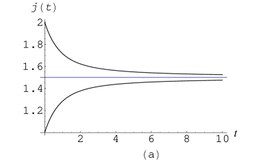
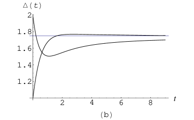
Figure 2: The tendency of current $j=Pv$ (a) and diffusion constant (b) to stationary values (the horizontal line) for $L=5$, $P=3$ in continuous time. The two branches correspond to different initial conditions.

As it is clearly seen, the velocity and the diffusion coefficient relax to their known stationary values, thus giving evidence of the correctness of the general expressions derived here. Although the concrete way of approach to stationarity depends strongly on the initial condition, the long-time relaxation seems to be exponential, at least for small systems.

IV Zeros of the partition function

¿From the equilibrium theory by Yang and Lee YL52 it is known that the zeros of the partition function of a finite-size system in the complex fugacity plane approach the real axis when the system size increases. By calculating the line of zeros in the thermodynamic limit, and their density near the real axis, one can exactly locate the transition point and obtain the order of the phase transition. Recently, essential progress has been made in the extension of the Lee-Yang theory to the non-equilibrium transitions between stationary states of the TASEP. Blythe and Evans BE02 , BE03 , found that the distribution of the zeros of the normalization factor for the continuous-time TASEP with open boundaries in the plane of complex injection rate agrees with the predictions of the Lee-Yang theory, see also BE04 . Exact mappings of the normalization factor for the discrete-time parallel update onto several equivalent two-dimensional lattice path problems were obtained in BJJK . The applicability of the concepts of finite-size scaling and universality with respect to the different types of updates for the open TASEP has been established in BB . For an overview on the recent breakthroughs in the extension of the Lee-Yang theory to non-equilibrium phase transitions we refer the reader to BDL .

Figure 3: Two configurations of paths are shown. The ovals surround different clusters of particles standing during tree time-steps: in part (a) the cluster of four standing particles contributes a total weight of $y^{3}$, and in part (b) the two clusters, of two standing particles each, contribute a total weight of $xy^{6}$.

Let us now re-interpret the generating function (11) as a partition function of a two-dimensional lattice path problem, in which the horizontal coordinates correspond to the original lattice sites, and the vertical direction is the discrete time. Each step to the right has a statistical weight $x=wz$, and each vertical step has a weight $y=(1-z)$ if the target site for the next step is empty and the weight 1 if it is occupied. Fig. 3 illustrates the equivalent two-dimensional path problem. The statistical weights $x,y,1$ are ascribed to all steps of the paths in accordance with the TASEP dynamics. In terms of these new variables, (11) takes the form of a polynomial $Z_{T}(x,y)$ with positive coefficients. For instance, the polynomial corresponding to $\Lambda_{3}(w,z)$ is

$$Z_{3}(x,y) = x^{9}+3x^{8}y+3x^{7}y(1+2y)+3x^{6}y(1+3y+2y^{2})+3x^{5}y^{2}(2+4y+y^{2})+x^{4}y^{2}(3+10y+7y^{2}+y^{3})$$ (19)

$$+ 3x^{3}y^{2}(1+2y+2y^{2}+y^{3})+3x^{2}y^{3}(1+y+y^{2})+xy^{3}(1+y+y^{2})+y^{3}.$$

Obviously, the probability normalization condition now implies $Z_{T}(x,1-x)\equiv 1$. Inspired by the success of the Lee-Yang theory in explaining how singularities may build up in the thermodynamic limit, we attempt to clarify the analytical structure of $Z_{T}(x,y)$ by studying the location of its zeros in the planes of complex fugacities $x$ and $y$, for sufficiently long times $T$, different ring sizes $L$ at fixed particle density $P/L$ and given initial conditions. The patterns of zeros obtained in the complex-$x$ and complex-$y$ planes are illustrated in Figs. 4 and 5, respectively, for three cases: $L=6$, $P=3$, $T=40$; $L=8$, $P=4$, $T=40$; and $L=10$, $P=5$, $T=30$.

Figure 4: The pattern of zeros of the partition function $Z_{T}(x,0.5)$ in the complex-$x$ plane for $L=6$, $P=3$, $T=40$ (solid squares), $L=8$, $P=4$, $T=40$ (open circles), and $L=10$, $P=5$, $T=30$ (open triangles). Note that the number of branches equals the number of particles $P$.

Figure 5: The pattern of zeros of the partition function $Z_{T}(0.5,y)$ in the complex-$y$ plane for $L=6$, $P=3$, $T=40$ (solid squares), $L=8$, $P=4$, $T=40$ (open circles), and $L=10$, $P=5$, $T=30$ (open triangles).

By inspecting these figures, one may speculate on the tendency of the zeros to approach the positive fugacity axis with increasing $L$ at fixed $P/L$. That may signal the appearance of a kind of condensation phase transition in the related thermodynamic model with fugacities $x$ and $y$. Arguments in favor of such a conjecture are given in the next section.

V Condensation

To reveal the nature of the possible phase transition, it is convenient to use the mapping of the TASEP onto the zero-range process (ZRP), see ZRP for a recent review. Consider a ZRP each site of which is identified, in the same sequential order, with one of the $L-P$ empty sites of the TASEP. Let the number of particles at each site of the ZRP be equal to the number of neighboring occupied sites of the TASEP just on the left of the corresponding empty site.

The interpretation of the partition function $Z_{T}(x,y)$ in terms of the ZRP is the following. Each jump of a particle from site $i$ to site $i+1$ $(i=1,2,\dots,L-P;i+L-P=i)$ for the unit time step from $t$ to $t+1$ carries a weight $x$, as in the TASEP. Each site occupied by least one particle which does not move during that time step has the weight $y$. The total contribution to $Z_{T}(x,y)$ from a particular realization of the process is the product of weights over all time steps from $0$ to $T$. Comparing the contributions with different factors $y^{n}$ and $y^{m}$, $n\leq m$, and equal number of spatial steps (i.e. factors $x^{k}$), we see that the decrease in $y$ leads to reduction in the average number of sites occupied by immobile particles and, therefore, to an effective clustering attraction between them. For sufficiently small $y$, i.e. sufficiently strong attraction, a condensation of particles may take place at a site (or at a number of sites).

Real-space condensation phenomena are known to take place in the stationary states of both the heterogeneous ZRP, with site-dependent hopping probabilities, and the homogeneous ZRP, where the hopping rates depend only on the occupation number of the departure site ZRP . In the former case the $P$ particles of the ZRP are viewed as bosons which may have $N=L-P$ energies determined by the different single-site hopping rates; the energy levels are defined so that the ground state corresponds to the lowest hopping rate. In the discrete-time TASEP with quenched random hopping probabilities of the particles Evans1 , the phase transition takes place between a low-density inhomogeneous phase, with a traffic jam behind the slowest particle (and empty space in front of it), and a high-density congested phase.

In our case the condensation is due to a specific interplay between the immobility probability $y$ and the fugacity $x$ associated with the hopping probability. Turning back to the effective two-dimensional path problem, we see that vertical bonds, corresponding to immobile neighboring particles, tend to form compact clusters, or jams in the TASEP traffic. This situation is shown in the ovals in Fig. 3. The cluster of four standing particles in Fig. 3 (a) lives three time steps and brings the total weight $y^{3}$. The configuration of paths in Fig. 3 (b) corresponds to two clusters containing two standing particles each. The weight of the configuration in the second oval is $xy^{6}$ that is much less than $y^{3}$ for small $y$. Varying parameters $x,y$, one may attain an arbitrary strong effective attraction between clusters.

VI Discussion

Here we considered the exact evolution of the TASEP on small rings during finite intervals of discrete time. The results for the velocity and diffusion constant are not surprising. As expected, both of them tend to their stationary values exponentially, although the particular features of the convergence depend on the initial conditions.

A more interesting object is the generating function of the process. Considering it as a function of two independent variables, fugacities of immobile particles and particle jumps, we studied the loci of its zeros in the planes of complex fugacities. When the location of the zeros in the right-hand half-plane is well behaved, a finite-size scaling analysis can provide important results concerning the very existence, the location, and the characteristics of the conjectured phase transition. However, the study of larger lattices and longer evolution times poses serious computational problems and will be presented in a forthcoming work. Although the tractable system sizes are too small, the obtained patterns suggest that with increasing the lattice size at a fixed particle density, the zeros may concentrate at a complex phase boundary which cuts the positive real axis at the transition point. When the corresponding fugacity crosses that point, a phase transition in the related two-dimensional equilibrium lattice path model should occur. We interpret this transition as a condensation of immobile particles. However, several problems remain unsolved.

The first one is to prove the existence of a phase transition in the framework of equilibrium statistical mechanics. To this end, one has to define an order parameter and a low-temperature phase which is destroyed when the temperature increases. If one succeeds in defining an interface between the phases, the proof can be based on contour arguments contour which compare the entropy and energy of the boundary of the low-temperature clusters.

The second problem is the kind of the phase transition. According to the Lee-Yang theory, it can be determined by evaluating the asymptotic density of zeros around the real axis. However, the fulfillment of this program needs consideration of much larger systems than the ones considered here.

It is of interest also to construct the complete phase diagram of the model in the $(z,w)$ plane, or in the $(x,y)$ plane, and to clarify the relationship between the dynamics of the TASEP and the thermodynamics of the effective two-dimensional model.

Appendix

Here we present the derivation of expression (16) for the stationary velocity in finite-size systems.

After summation over all final configurations $C$, Eq. (15) can be written as a sum over all clusters (connected sequences of neighboring particles) in the initial configuration $C^{0}$:

$$v_{st}=\frac{1}{P}{L\choose{P}}^{-1}\frac{z}{1-z}\sum_{C^{0}}\sum_{i=1}^{m(C^{0})}\left(1-z^{N_{i}(C^{0})}\right),$$ (20)

where $m(C^{0})$ is the number of clusters in configuration $C^{0}$ and $N_{i}(C^{0})$ is the number of particles in the $i$-th cluster of the configuration $C^{0}$. For further calculations, it is convenient to introduce the following generating function of the stationary velocity:

$$\Gamma(L,z,s)=\sum_{P=1}^{L-1}P{L\choose{P}}v_{st}(L,P,z)s^{P}.$$ (21)

It is readily seen that the stationary TASEP can be mapped on the Fortuin-Kasteleyn representation of the one-dimensional Potts model with external field Fortuin . To this end, we introduce the ring graph $G$ with $L$ vertices located at the centers of the bonds of the TASEP ring $R$. Let $G^{\prime}$ be a subgraph of $G$, such that two neighboring vertices are connected by an edge if and only if the common site of the corresponding bonds of $R$ is occupied. Thus, we obtain a one-to-one correspondence of the TASEP configurations on $R$ and the subgraphs of $G$. Note that the graph $G$ itself and the edgeless subgraph correspond to the fully occupied $(P=L)$ and the empty $(P=0)$ rings, respectively. The velocity generating function (21) can be represented as a sum over all subgraphs:

$$\Gamma(L,z,s)=\frac{z}{1-z}\sum_{G^{\prime}\subseteq G}s^{e(G^{\prime})}\sum_{i=1}^{k(G^{\prime})}\left(1-z^{n_{i}(G^{\prime})-1}\right)-\frac{z}{1-z}\left(1-z^{L-1}\right)s^{L},$$ (22)

where $e(G^{\prime})$ and $k(G^{\prime})$ are correspondingly the number of edges and the number of connected components of $G^{\prime}$, $n_{i}(G^{\prime})$ is the number of vertices in the $i$-th connected component of $G^{\prime}$. The last therm is a correction to the fully occupied case. The partition function of the $q$-state Potts model in external field can be expanded over the spanning subgraphs as follows:

$$\mathcal{Z}_{Potts}(q,v,w)=\sum_{G^{\prime}\subseteq G}v^{e(G^{\prime})}\prod_{i=1}^{k(G^{\prime})}\left[(w+1)^{n_{i}(G^{\prime})}+q-1\right].$$ (23)

Here $v$ and $w$ are the coupling and external field parameters, respectively. If we denote

$$f(v,w)=\frac{1}{(w+1)^{L}}\left.\frac{\partial\,\mathcal{Z}_{Potts}}{\partial q}\right|_{q=1},$$ (24)

then the generating function (22) can be written as

$$\Gamma(L,z,s)=\frac{z}{1-z}f(s,0)-\frac{1}{1-z}f(s,\frac{1-z}{z})-\frac{z}{1-z}\left(1-z^{L-1}\right)s^{L}.$$ (25)

By using the exact expression for the Potts model partition function,

$$\mathcal{Z}_{Potts}(q,v,w)=(q-2)v^{L}+(\lambda^{+})^{L}+(\lambda^{-})^{L},$$ (26)

with

$$\lambda^{\pm}=\frac{1}{2}\left[q+2v+w+vw\pm\sqrt{(q+2v+w+vw)^{2}-4v(q+v)(1+w)}\right],$$ (27)

after some simplifications we find

$$\Gamma(L,z,s)=Lzs\frac{(1+s)^{L-1}-(zs)^{L-1}}{1+s-zs}.$$ (28)

With the aid of the above exact expression we obtain the explicit expression (16) for the stationary velocity.

References

- (1) T. M. Liggett, Interacting Particle Systems (Springer, 1985).
- (2) H. Spohn, Large Scale Dynamics of Interacting Particles (Springer, 1991).
- (3) D. Dhar, Phase Trans. 9, 51 (1987).
- (4) L. H. Gwa and H. Spohn, Phys. Rev. Lett. 68, 725 (1992).
- (5) B. Derrida, M. R. Evans, and D. Mukamel, J. Phys. A 26, 4911 (1993).
- (6) S. A. Janovsky and J. L. Lebowitz, Phys. Rev. A 45, 618 (1992).
- (7) B. Derrida and K. Mallick, J. Phys. A 30, 1031 (1997).
- (8) B. Derrida, Phys. Rep. 301, 65 (1998).
- (9) B. D. Derrida and J.L. Lebowitz, Phys. Rev. Lett. 80, 209 (1998).
- (10) G. M. Schütz, J. Stat. Phys. 88, 427 (1997).
- (11) V. B. Priezzhev, Phys. Rev. Lett. 91, 050601 (2003).
- (12) M. R. Evans, J. Phys. A 30, 5669 (1997).
- (13) N. Rajewsky, L. Santen, A. Schadschneider and M. Schreckenberg, J. Stat. Phys. 92, 151 (1998).
- (14) C. N. Yang and T. D. Lee, Phys. Rev. 87, 404 (1952).
- (15) R. A. Blythe and M. R. Evans, Phys. Rev. Lett. 89, 080601 (2002).
- (16) R. A. Blythe and M. R. Evans, Braz. J. Phys. 33, 464 (2003).
- (17) R. Brak and J. W. Essam, J. Phys. A 37, 4183 (2004).
- (18) R.A. Blythe, W. Janke, D.A. Johnston, and R. Kenna, J. Stat. Mech.: Theory and Exper. P06001 (2004); cond-mat/0405314 (2004).
- (19) J. Brankov and N. Bunzarova, Phys. Rev. E 71, 036130 (2005).
- (20) I. Bena, M. Droz, and A. Lipowski, arXiv: cond-mat/0510278 (2005).
- (21) M. R. Evans and T. Hanney, J. Phys. A 38, R195 (2005).
- (22) R. Peierls, Proc. Cambridge Philos. Soc. 32, pt. 3, 447 (1936).
- (23) M. Biskup, C. Borgs, J. T. Chayes, L. J. Kleinwaks, and R. Kotecky, Phys. Rev. Lett. 84, 4794 (2000).
- (24) P. W. Kasteleyn and C. M. Fortuin, J. Phys. Soc. Jpn. Suppl. 26, 11 (1969); C. M. Fortuin and P. W. Kasteleyn, Physica 57 536 (1972).