Glassy dynamics and nonextensive effects in the HMF model: the importance of initial conditions

Abstract

We review the anomalies of the HMF model and discuss the robusteness of the glassy features vs the initial conditions. Connections to Tsallis statistics are also addressed.

1 Introduction

In this work we discuss glassy dynamics and nonextensive thermodynamics in the context of the so called Hamiltonian Mean Field (HMF) model, a system of inertial spins with long-range interaction. This model and its generalizations has been intensively investigated in the last years for its anomalous dynamical behavior [1, 2, 3, 4, 5, 6, 7, 8, 9, 10, 11, 12, 13]. With respect to systems with short-range interactions, the dynamics and the thermodynamics of many-body systems of particles interacting with long-range forces, as the HMF, are particularly rich and interesting.

The Hamiltonian Mean Field model is exactly solvable at equilibrium, but exhibits a series of anomalies in the dynamics, as the presence of quasistationary states (QSS) characterized by: anomalous diffusion, vanishing Lyapunov exponents, non-gaussian velocity distributions, aging and fractal-like phase space structure. Thus, it represents a very useful “laboratory” for exploring metastability and dynamical anamalies in systems with long-range interactions. The model can be considered as a pedagogical model for a large class of complex systems, among which one can surely include self-gravitating [12] and glassy systems [9], but also systems apparently belonging to different fields as biology or sociology. Similar features were recently found also in the context of the Kuramoto model [19], one of the simplest models for synchronization in biological systems [20]. Moreover, the proliferation of metastable states in the vicinity of a critical point in the phase diagram seems to be quite a general feature  [18] .
In this paper we focus on two different aspects of the HMF model: its glassy-dynamics and the possible connections with the generalized thermodynamics. We will study in particular the dependence of these features on the initial conditions considered.

2 Out-of-equilibrium dynamical anomalies

The Hamiltonian of the HMF model is given by

$$H=K+V=\sum_{i=1}^{N}\frac{p_{i}^{2}}{2}+\frac{1}{2N}\sum_{i,j=1}^{N}[1-\cos(\theta_{i}-\theta_{j})]~{}~{}~{}~{}.$$ (1)

This Hamiltonian describes classical $XY$-spins (or rotators) with unitary mass and infinite range coupling, but it can also represent particles moving on the unit circle. In the latter case the coordinate $\theta_{i}$ of the $i-th$ particle is its position on the circle and $p_{i}$ is its conjugate momentum (or angular velocity). The potential energy term is rescaled by $1/N$ in order to get a finite energy density in the thermodynamic limit $N\rightarrow\infty$  [1, 2]. Associating to each particle the spin vector $\overrightarrow{s}_{i}=(\cos\theta_{i},\sin\theta_{i})~{}~{}$, one can introduce the following mean-field order parameter $M=\frac{1}{N}|\sum_{i=1}^{N}\overrightarrow{s}_{i}|~{}~{}$, which is the modulus of the total magnetization.
At equilibrium the exact solution predicts a second-order phase transition. The system passes as a function of energy from a low-energy condensed (ferromagnetic) phase with magnetization $M\neq 0$, to a high-energy one (paramagnetic), where the spins are homogeneously oriented on the unit circle and $M=0$. The caloric curve, i.e. the dependence of the energy density $U=H/N$ on the temperature $T$, is given by $U=\frac{T}{2}+\frac{1}{2}\left(1-M^{2}\right)~{}~{}$[1, 4] . The critical point is found at a temperature $T_{c}=0.5$, which corresponds to the critical energy density $U_{c}=0.75$.
At variance with the equilibrium scenario, the out-of-equilibrium dynamics shows, just below the phase transition, several anomalies before equilibration. More precisely, starting from water bag initial conditions in the momenta, i.e. velocities uniformly distributed, and a fully magnetized state, i.e. all the $\theta_{i}=0$ so that M(0)=1, the results of the simulations, in a special region of energy values (in particular for $0.68<U<U_{c}$) show a disagreement with the equilibrium prediction for a transient regime whose length depends on the system size N. In such a regime the system remains trapped in metastable quasi-stationary states (QSS) with vanishing magnetization at a temperature lower then the equilibrium one and shows strong memory effects, correlations and aging. Then it slowly relaxes towards Boltzmann-Gibbs (BG) equilibrium. This transient QSS regime becomes stable if one takes the infinite size limit before the infinite time limit [5] .

2.1 Hierarchical structures and glassy dynamics

In order to investigate the nature of this trapping phenomenon, it is interesting to explore directly the microscopic evolution of the QSS. A way to visualize it is by plotting the time evolution of the Boltzmann $\mu$-space: each particle of the system is represented by a point in a plane characterized by the conjugate variables $\theta_{i}$ and $p_{i}$. It has been shown[7] that, during the QSS regime, correlations, structures and clusters formation in the $\mu$-space appear for the $M(0)=1$ initial conditions ($M1~{}ic$), but not for initial conditions with zero initial magnetization ($M0~{}ic$). In fact, while the former case is characterized by a sudden quenching from an high temperature state that causes a strong mixing of particles in the metastable regime, in the latter case no quenching is present: both the angles and velocities distributions remain homogeneous from the beginning and a very slow mixing of the particles can be observed.

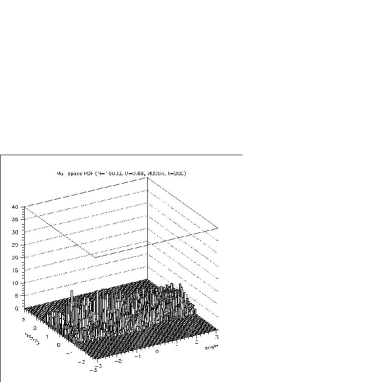
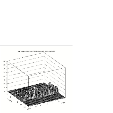
Figure 1: For the energy density $U=0.69$, $N=10000$ and for different initial conditions we plot a snapshot of the $\mu-space$ at time $t=200$ inside the plateau regime. The figure illustrates four different initial magnetization cases, M=1 (top-left), M=0.95 (top-right), M=0.8 (bottom-left) and M=0 (bottom right). Competing clusters of different sizes are clearly visible only for the case M=1. See text for further details.

For the $M1ic$ case, the dynamics in $\mu$-space can be also clarified through the concept of ”dynamical frustration”: the clusters appearing and disappearing on the unit circle compete one with each other in trapping more and more particles, thus generating a dynamically frustrated situation typical of glassy systems [9]. In Fig.1 we show the dependence of the competing clusters phenomenon as a function of the initial magnetization. The distribution function $f(\theta,p,t)$ is considered for different out of equilibrium initial conditions (i.c.) inside the QSS regime. In particular for N=10000 and U=0.69 we plot a snapshot of the $\mu$-space configuration at $t=200$ for four initial magnetizations, namely M=1, M=0.95, M=0.8 and M=0, obtained by spreading the initial angles distribution over a wider and wider portion of the unit circle. In this way we fix the initial potential energy $V(\theta)$ and, in turn, the magnetization. Then, we assign the remaining part of the total energy as kinetic energy by using a water bag uniform distribution for the velocities.

We define each cluster as composed by particles with both angles and velocities in the same $\mu$-space cell. A total of 100x100 cells for the $\mu$-space lattice has been considered. In Fig.1 one clearly observes the presence of competing clusters only for M=1 i.c.. At variance already for M=0.95 i.c. clusters are not very evident and the configuration tends to become more and more uniform decreasing the initial magnetization. These simulations show that, although dynamical structures are present in the QSS regime up to M=0.4 [10], frustration due to competing clusters seems to depend much more strictly on the initial quenching which is very violent for M=1 i.c..

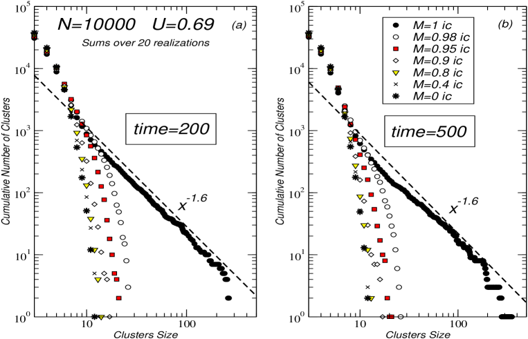
Figure 2: We plot for the case $U=0.69$ and $N=10000$ the cumulative distribution of the clusters size, calculated for time $t=200$, panel (a), and $t=500$, panel (b), in the QSS region. The points refers to different initial conditions: while the initial momenta were always uniformly ditributed, the initial magnetizations changed as reported in the legend. A power law can be observed only for initial magnetization M=1, black circles. A decaying power law with exponent $-1.6$ is also reported for comparison as dashed curve. See text.

In order to give further support to this result, in Fig. 2 we show the behavior of the cluster size cumulative distributions calculated in the case N=10000 and U=0.69 for several initial magnetizations in the QSS regime at time t=200, panel (a), and t=500, panel (b). For each one of the 100x100 $\mu$-space cells a sum over 20 different realizations of the dynamics (events) has been performed. Then, for each cluster size (greater than 5 particles) the sum of all the clusters with equal of bigger size has been calculated and plotted.
As one can see from Fig.2 a power law distribution, which indicates the presence of a hierarchical structure, can be observed only for initial conditions with $M=1$. In all the other cases studied, i.e. for initial magnetization smaller or equal to $M=0.95$ the power law disappears. By comparing panel (a) with panel (b) one can also notice that, as expected, the distributions does not change significatively in time in the plateaux region. In the figure, we report also a power law fit (drawn as a straight dashed line above the data points) for the M=1 case: for both cases at t=200 and at t=500, the cluster size distribution has an exponent decay approximately equal to $-1.6$.
Such a strong dependence of the clusters hierarchical structure on the initial conditions confirms that, although a metastable macroscopic regime is observed in all cases, the microscopic structure of correlations is deeply different. The cluster size distribution observed for M=1 i.c. reminds closely that of percolation at the critical point, where a lenght scale, or time scale, diverges leaving the system in a self-similar state [22]. More in general, it has been suggested [23] that, optimizing Tsallis’ entropy with natural constraints in a regime of long-range correlations, it is possible to derive a power-law hierarchical cluster size distribution which can be considered as paradigmatic of physical systems where multiscale interactions and geometric (fractal) properties play a key role in the relaxation behavior of the system. The power-law scaling strongly suggests a non-ergodic topology of the region of phase space in which the system remains trapped when the QSS regime is reached.

These results also supports the so called ”weak ergodicity-breaking” scenario typical of glassy systems. In ref.[24] such a mechanism has been proposed in order to explain the aging phenomenon, i.e. the dependence of the relaxation time on the history of the system[17]. Aging has been found also in the HMF model for $M1$ i.c., more precisely in the autocorrelation functions decay for both the angles and velocities [8] and for velocities only [7]. More recently, inspired by the physical meaning of the Edwards-Anderson spin-glass order parameter [25], we proposed a new order parameter for the HMF model, with the aim to measure the degree of freezing of the rotators in the QSS regime and to characterize in a quantitative way the emerging glassy-like dynamics [9].

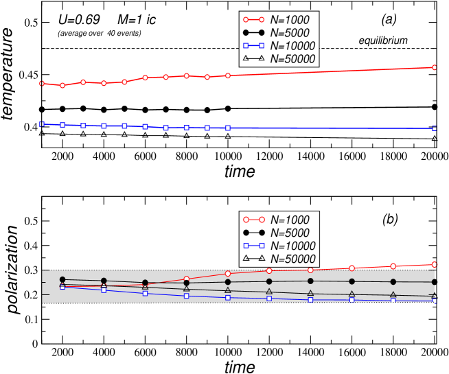
Figure 3: For the energy density $U=0.69$ and different sizes (N=1000,5000,10000,50000), we plot the time evolution of the temperature for different initial magnetizations in panel (a). In panel (b), we show the corresponding polarization values obtained for $\tau=2000$ and for increasing times along the QSS plateau. The latter seems to be quite constant in time and with a value $0.24\pm 0.05$. We plot a grey zone to illustrate these limits of variation. Notice that for N=1000 the the temperature start to relax towards the equilibrium value around t=5000, so also the polarization tends to increase.

We define the elementary polarization as the temporal average, integrated over an opportune time interval $\tau$, of the successive positions of each rotator:

$$<\stackrel{{\scriptstyle\vector(1,0){8.0}}}{{s_{i}}}>={1\over{\tau}}\int_{t_{0}}^{t_{0}+\tau}\stackrel{{\scriptstyle\vector(1,0){8.0}}}{{s_{i}}}(t)dt~{}~{}~{}~{}~{}~{}i=1,...,N~{}~{},$$ (2)

being $t_{0}$ an initial transient time. Then we average the module of the elementary polarization over the N rotators, to obtain the polarization p:

$${\it p}={1\over{N}}\sum_{i=1}^{N}|<\stackrel{{\scriptstyle\vector(1,0){8.0}}}{{s_{i}}}>|~{}~{}~{}~{}.$$ (3)

It is important to point out that, in order to calculate the elementary polarization of eq.2, one has to subtract the global motion of the system, i.e. the phase of the average magnetization, from the phase of each rotator.
By means of several numerical simulations we showed in ref.[9] that in the QSS regime for $0.68<U<0.75$ and $M1ic$, the polarization is constant and greater than zero - inside the error representing the fluctuations of the elementary polarization module - while the magnetization vanishes with the size of the system. Thus the polarization can be really considered a new order parameter able characterize the glassyness of the QSS regime [9] .

In Fig.3 we present new calculations for $U=0.69$ and $M=1$ initial conditions. In panel (a) we report the time evolution of temperature for different sizes of the system ($N=1000$, $N=5000$, $N=10000$ and $N=50000$) and after a transient $t_{0}=1000$. In panel (b) we plot the corresponding polarization calculated at different times and for a time interval $\tau=2000$. One can see that the polarization remains almost constant around a value $p=0.24$ and inside an error of $\pm 0.05$ (grey area in the figure), it does not change substantially inside the QSS temperature plateaux and does not depend within the error on the size of the system. In general the length of the plateaux regime depends on the size of the system, thus the integration time $\tau=2000$ has been chosen in order to make a meaningful calculation for all the sizes, included the smaller one ($N=1000$).

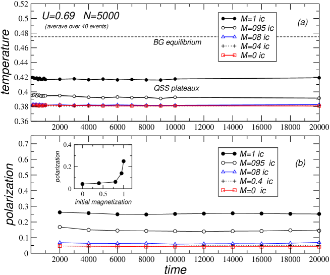
Figure 4: For the energy density $U=0.69$ and N=5000, we plot the time evolution of the temperature for different initial conditions for the magnetization in panel (a). In panel (b), we show the corresponding polarization increasing the time interval of calculation. The polarization seems to depend strongly on the initial conditions and tends rapidly to zero as a function of the initial magnetization as reported in the inset. See text for further details.

In Fig.4 we compare the calculation of the polarization obtained for $U=0.69$, $N=5000$ and different initial magnetizations i.e. $M=1,0.95,0.8,0.4,0$. We report in panel (a) the temperature time evolution, while in panel (b) we plot the corresponding polarization as a function of time. Also in this case a time interval $\tau=2000$ has been considered to calculate the polarization. The plots are in agreement with the previous results about the $\mu$-space cluster distributions. In fact also the polarization seems to be strongly dependent on the initial conditions and rapidly tends to zero by decreasing the initial magnetization, as reported in the inset of panel (b). Again, the fast initial quenching we observe for the M=1 i.c. confirms its key role in generating glassy behaviour in HMF model. On the other side, as we will show in the next subsection, nonextensive features are quite more robust and seems to be less sensible to the initial magnetization.

2.2 Nonextensive thermodynamics and HMF model

In previous works it was shown that the majority of the dynamical anomalies of the QSS regime, among which velocity correlations in the $\mu$-space, are present not only for $M1$ initial conditions, but also when the initial magnetization $M(t=0)$ is decreased in the range $(0,1]$ [10].
The velocity correlations can be calculated by using the following autocorrelation function[10]

$${C}(t)=\frac{1}{N}\sum_{j=1}^{N}{p_{j}(t)p_{j}(0)}~{}~{},$$ (4)

where $p_{j}(t)$ is the velocity of the $j$-th particle at the time $t$. In Fig.5, we plot the velocity autocorrelation function (4) for $N=1000$, $U=0.69$ and $M(0)={1,0.8,0.6,0.4,0.2,0}$. An ensemble average over 500 different realizations was performed. For $M(0)\geq 0.4$ the correlation functions are very similar, while the decay is faster for $M(0)=0.2$ and even more for $M(0)=0$. If we fit these relaxation functions by means of the Tsallis’ q-exponential function

$$e_{q}(z)={\left[1+(1-q)z\right]}^{\frac{1}{(1-q)}}~{}~{},$$ (5)

with $z=-\frac{t}{\tau}$, and where $\tau$ is a characteristic time, we can quantitatively discriminate between the different initial conditions. In fact we get a q-exponential with $q=1.5$ for $M(0)\geq 0.4$, while we get $q=1.2$ and $q=1.1$ for $M(0)=0.2$ and for $M(0)=0$ respectively. Notice that for $q=1$ one recovers the usual exponential decay [15, 4, 5, 7]. Thus for $M(0)>0$ correlations exhibit a long-range nature and a slow power-law decay. This decay is very similar for $M(0)\geq 0.4$, but diminishes progressively below $M(0)=0.4$ to become almost exponential for $M(0)=0$.
Velocity correlations seem to be linked to anomalies in the diffusion. In order to study diffusion, one can consider the mean square displacement of phases $\sigma^{2}(t)$ defined as

$$\sigma^{2}(t)=\frac{1}{N}\sum_{j=1}^{N}[\theta_{j}(t)-\theta_{j}(0)]^{2}=<[\theta_{j}(t)-\theta_{j}(0)]^{2}>~{},$$ (6)

where the symbol $<...>$ represents the average over all the $N$ rotators. The quantity $\sigma^{2}(t)$ typically scales as $\sigma^{2}(t)\sim t^{\gamma}$. The diffusion is normal when $\gamma=1$ (corresponding to the Einstein’s law for Brownian motion) and ballistic for $\gamma=2$ (corresponding to free particles). For different values of $\gamma$ the diffusion is anomalous, in particular for $1<\gamma<2$ one has superdiffusion. We notice that the quantity $\sigma^{2}(t)$ can be rewritten by using the velocity correlation function $C(t)$ as

$$\sigma^{2}(t)=\int_{0}^{t}dt_{1}\int_{0}^{t}dt_{2}~{}<p_{j}(t_{2})~{}p_{j}(t_{1})>\\ =2\int_{0}^{t}dt_{1}\int_{0}^{t_{1}}dt_{2}~{}C(t_{2})~{}~{}~{},$$ (7)

where $C(t)$ is defined as in Eq.4.

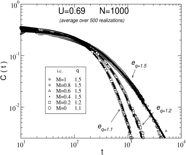
Figure 5: For the energy density $U=0.69$ and N=1000, we plot the time evolution of the correlation function $C(t)$ for different initial magnetization. A q-exponential fit is also reported for each curve See text for further details.

Superdiffusion has been already observed in the HMF model for M1 initial conditions[3]. Rercently we have also checked that, even decreasing the initial magnetization, the system continues to show superdiffusion [10]. In particular we obtained an ananoalous diffusion exponent that goes progressively from $\gamma=1.4-1.5$ for $0.4<M(0)<1$ to $\gamma=1$ for M0  [13]. No sensitive dependence on the size of the system has been orserved. The slow decay and the superdiffusive behavior can be connected by means of a conjecture based on a theoretical result found in ref.[21] by Tsallis and Bukman. In fact in that paper the authors show, on general grounds, that nonextensive thermostatistics constitutes a theoretical framework within which the unification of normal and correlated (driven) anomalous diffusions can be achieved. They obtain, for a generic linear force $F(x)$, the physically relevant exact (space, time)-dependent solutions of a generalized Fokker-Planck equation. Following ref.[21], it is possible to recover this relationship

$$\gamma=\frac{2}{3-q}~{},$$ (8)

between the exponent $\gamma$ of anomalous diffusion and the entropic index $q$. Hence, being the space-time distributions linked to the respective velocity correlations by the eq. (7), one could think to insert in eq. (8) the entropic index $q$, characterizing the correlation decay and the corresponding anomalous diffusion exponent. In order to check this conjecture, we have studied the ratio $\frac{\gamma}{2/(3-q)}$ vs the exponent $\gamma$ for various initial conditions ranging from M(0)=1 to M(0)=0 and different sizes at $U=0.69$ . Within an uncertainty of $\pm 0.1$, the data [13] (not reported here for lack of space) show that this ratio is always one, thus providing a strong indication in favor of this conjecture. Although rigorous results are still missing the numerical evidence here discussed indicate that Tsallis statistics and in particular its entropic index $q$ seems to be able to give a quantitative characterization of the correlations and dynamical anomalies found in the QSS regime of the HMF model.

3 Conclusions

We have briefly reviewed some of the anomalous features oberved in the dynamics of the HMF model, a kind of minimal model for the study of complex behavior in systems with long-range interactions. We have also discussed how the anomalous behavior can be interpreted within the nonextensive thermostatistics introduced by Tsallis, and in the framework of the theory glassy systems. These two frameworks seems to have several links which will be further explored in the future.

References

- [1] M. Antoni and S. Ruffo, Phys. Rev. E 52, 2361 (1995).
- [2] T. Dauxois, V. Latora, A. Rapisarda, S. Ruffo and A. Torcini, Dynamics and Thermodynamics of Systems with Long Range Interactions, T. Dauxois, S. Ruffo, E. Arimondo, M. Wilkens Eds., Lecture Notes in Physics Vol. 602, Springer (2002) p. 458 and refs. therein.
- [3] V. Latora, A. Rapisarda and S. Ruffo, Phys. Rev. Lett. 83 (1999) 2104
- [4] A. Pluchino, V. Latora, A. Rapisarda, Continuum Mechanics and Thermodynamics 16, 245 (2004) and refs therein.
- [5] C. Tsallis, A. Rapisarda, V. Latora and F. Baldovin, Dynamics and Thermodynamics of Systems with Long Range Interactions, T. Dauxois, S. Ruffo, E. Arimondo, M. Wilkens Eds., Lecture Notes in Physics Vol. 602, Springer (2002) p.140 and refs therein.
- [6] For a generalized version of the HMF model see: C. Anteneodo and C. Tsallis, Phys. Rev. Lett. 80, 5313 (1998); F. Tamarit and C. Anteneodo,Phys. Rev. Lett. 84, 208 (2000); A. Campa, A. Giansanti, D. Moroni, Phys. Rev. E 62, 303 (2000) and Physica A 305, 137 (2002) B.J.C. Cabral and C. Tsallis Phys. Rev. E, 66 065101(R) (2002).
- [7] A. Pluchino, V. Latora, A. Rapisarda, Physica D 193, 315 (2004).
- [8] M.A.Montemurro, F.A.Tamarit and C.Anteneodo, Phys. Rev. E 67, 031106 (2003).
- [9] A. Pluchino, V. Latora, A. Rapisarda Phys. Rev. E 69 (2004) Physica A 340, 187 (2004) Glassy order parameter for the HMF model cond-mat/0506665, submitted to Phys.Rev.E
- [10] A. Pluchino, V. Latora, A. Rapisarda, Physica A 338, 60 (2004).
- [11] Y. Yamaguchi, J.Barré, F.Bouchet, T.Dauxois and S.Ruffo, Physica A 337, 653 (2004).
- [12] P.H. Chavanis, J. Vatterville and F. Bouchet, cond-mat/0408117.
- [13] A. Pluchino, V. Latora, A. Rapisarda, proceeding of the international conference ”Complexity, Metsatsbility and Nonextensivity”, eds. C.Beck, G.Benedek, A. Rapisarda and C Tsallis, World Scientific (2005) cond-mat0507005.
- [14] C.Tsallis, J.Stat.Phys. 52, 479 (1988).
- [15] Nonextensive Entropy: interdisciplinar ideas, C. Tsallis and M. Gell-Mann Eds., Oxford University Press (2004).
- [16] A. Cho, Science 297, 1268 (2002); S. Abe, A.K. Rajagopal; A. Plastino; V. Latora, A. Rapisarda and A. Robledo, Science 300, 249 (2003).
- [17] M.Mézard, G.Parisi and M.A.Virasoro,Spin Glass Theory and Beyond, World Scientific Lecture Notes in Physics Vol.9 (1987); J.P.Bouchaud, L.F.Cugliandolo, J.Kurchan and M.Mézard, Spin Glasses and Random Fields, ed.A.P.Young, World Scientific, (1998) Singapore.
- [18] M.Mézard, G.Parisi and R. Zecchina, Science 297, 812 (2002).
- [19] Y. Kuramoto, in it International Symposium on Mathematical Problems in Theoretical Physics, Vol. 39 of Lecture Notes in Physics, edited by H. Araki (Springer-Verlag, Berlin, 1975); Chemical Oscillations, Waves, and Turbulence (Springer-Verlag, Berlin, 1984).
- [20] A. Pluchino, V. Latora, A. Rapisarda, Metastability hindering synchronization in HMF and Kuramoto models (2005) in preparation.
- [21] C. Tsallis and D.J. Bukman, Phys. Rev. E 54,R2197 (1996).
- [22] J.J.Binney, N.J.Dowrick, A.J.Fisher,and M.E.J.Newman, The Theory of Critical Phenomena, Oxford Science Publications (1992).
- [23] Sotolongo-Costa O., Rodriguez Arezky H. and Rodgers G.J., Entropy 2 (2000) 77; Sotolongo-Costa O., Rodriguez Arezky H. and Rodgers G.J., Physica A A286 (2000) 638;
- [24] J.P.Bouchaud Weak ergodicity breaking and aging in disordered systems J.Phis.I France 2 (1992)
- [25] S.F.Edwards, P.W.Anderson, J.Phys.F 5, 965 (1975). D. Sherrington and S. Kirkpatrick, Phys. Rev. Lett. 35, (1975) 1792 D. Sherrington and S. Kirkpatrick, Phys. Rev. B 17 (1978) 4384.