Microcanonical solution of the mean-field model: comparison with time averages at finite size
Abstract
We solve the mean-field model in an external magnetic field in the microcanonical ensemble using two different methods. The first one is based on Rugh’s microcanonical formalism and leads to express macroscopic observables, such as temperature, specific heat, magnetization and susceptibility, as time averages of convenient functions of the phase-space. The approach is applicable for any finite number of particles . The second method uses large deviation techniques and allows us to derive explicit expressions for microcanonical entropy and for macroscopic observables in the limit. Assuming ergodicity, we evaluate time averages in molecular dynamics simulations and, using Rugh’s approach, we determine the value of macroscopic observables at finite . These averages are affected by a slow time evolution, often observed in systems with long-range interactions. We then show how the finite time averages of macroscopic observables converge to their corresponding values as is increased. As expected, finite size effects scale as .
keywords:
Microcanonical ensemble; Mean-field models; Finite size effects PACS: 05.20.-y, 05.20.Gg, 05.70.Fh1 Introduction
The microcanonical ensemble can be considered, in several respects, as the basic ensemble for the description of the statistical behavior of physical systems. However, the canonical ensemble is often more amenable to exact or approximate analytical treatments and, therefore, several calculations are usually performed in its framework. On the other hand, there are some reasons of principle, and also of practical importance, for which the microcanonical ensemble must be given a prominent role [1]. Indeed, there is an increasing evidence that ensembles can be nonequivalent for systems with long-range interactions [2] or for finite (small) systems, when surface effects are relevant [1, 3]. In the mathematical physics literature, this question has been first discussed in the pioneering paper by Hertel and Thirring [4] (a recent publication where several references to these results can be found is Ref. [5]). An alternative approach, in which a parallel study of the distributions of microstates and macrostates is performed, has been proposed in Ref. [6]. This approach is based on large deviation techniques [7].
On the other hand, it has been shown that inequivalence between microcanonical and canonical ensembles can be associated to the presence of first order phase transitions in the canonical ensemble [8], and that there are regions in the phase diagram of the system that can be reached only within the framework of the microcanonical ensemble [9, 10, 11]. This means that in such cases, preparing the system at either fixed energy or temperature determines different values of the macroscopic observables. It has been correctly pointed out that this implies the impossibility of defining a unique equation of state for the system [3]. Moreover, in systems with long-range forces or in small systems, when the interaction between macroscopic subsystems cannot be reduced to a surface effect, the very concept of a heat bath can be seriuously questioned [12].
The physical consequences of ensemble inequivalence are of paramount importance. Perhaps, the most striking example is the existence of negative specific heat in the microcanonical ensemble for self-gravitating systems [13] . This reflects the real physical situation, and, in the canonical ensemble, negative specific heat is simply impossible. Experimental observations of negative specific heat for atomic and molecular clusters have also been recently reported [14, 15].
The above arguments, which are all consequences of ensemble inequivalence, justify the necessity to perform, at least in some cases, microcanonical ensemble calculations. The operative problem then arises on how this can be actually done. This question can be faced both in the thermodynamic limit and at a finite number of degrees of freedom. The study of finite is relevant in two respects: in Molecular Dynamics (MD) simulations one would like to estimate the approach to the limit in numerical experiments, finite (small) systems, as just noted, can be interesting by themselves.
In this paper we discuss two different approaches to the study of a physical system within the framework of the microcanonical ensemble. We will consider the mean-field model in an external magnetic field. We will here restrict to the description of the solution methods and to the implementation of the expressions we obtain for macroscopic observables in MD simulations. We will not discuss issues directly related to ensemble inequivalence, which will be the subject of a forthcoming publication [16].
In Section 2 we review two different approaches to the calculation of microcanonical averages. The first one is based on the microcanonical formalism introduced by Rugh [17, 18]. The second [19] relies on large deviations techniques, which are particularly suited for mean-field like systems. In Section 3 we present and briefly discuss the model. In Section 4 we show how the two approaches can be applied to the model. In Subsection 4.1 we derive the finite formulas for some observables in Rugh’s microcanonical formalism, while in Subsection 4.2 large deviations techniques are used to compute the entropy of the system, and, from it, the expressions of the thermodynamic observables. We then show that the large limit of the microcanonical formalism gives the same results as the large deviation approach. In Section 5 we present the results of MD simulations of our model, with the aim of illustrating the approach to the limit. Section 6 is devoted to some conclusions and perspectives.
2 Two ways of obtaining microcanonical averages
In the computation of the entropy and of the averages of observables, the problem at hand is the calculation of integrals of functions of the phase space, restricted to a given energy shell, and of the dependence of these integrals on the energy. Here we consider two procedures that are somewhat complementary. They have been recently introduced in the literature (Refs. [17, 18] for the finite approach and Refs. [19, 20] for the large deviation one), and our aim is here to make a comparison between them, both as far as general aspects are concerned, and for the actual implementation in a specific case.
Rugh’s microcanonical formalism [17, 18] is in principle more general, since it is formulated for general Hamiltonians and for any number of degrees of freedom . It does not allow to obtain the entropy itself, but it gives access to averages of the observables and to derivatives of the entropy and of the averages with respect to the energy and to the parameters of the Hamiltonian. These derivatives are in turn expressed as averages of suitable observables, which must be determined otherwise, e.g. numerically. On the other hand, the large deviation method [19, 20] is mostly applicable to systems with long-range interactions. Expressions are obtained in the thermodynamic limit, although finite corrections can in principle be derived as series in . Its advantage is the possibility to actually compute the entropy itself, besides its derivatives, and to obtain analytically features of the limit, like phase transitions.
2.1 Rugh’s microcanonical averages
In this Subsection we review the basic expressions for the averages of observables in the microcanonical ensemble, as given in Refs. [17, 18]. We restrict to the case in which the total energy is the only integral of motion, and we consider a Hamiltonian that can depend on a parameter .
In units where the Boltzmann constant is equal to , the microcanonical volume is given by:
| (1) |
where denotes the phase space of the system, and the parameter the Hamiltonian depends on. The average of an observable is:
| (2) |
It is possible to express in turn the derivatives with respect to and of and of (and thus also the temperature) as averages. It is useful to introduce the notation
| (3) |
The derivatives of the function with respect to and can be expressed using any vector in space such that (where are the phase space variables and the gradient operator acts on ). Using the property
| (4) | |||||
one gets
| (5) | |||||
where we have integrated by parts. Moreover,
| (6) | |||||
The entropy and the average are expressed, through the use of (3), by
| (7) |
From Eqs. (5), (2.1) and (2.1) it follows that
| (8) |
| (9) |
| (10) |
| (11) | |||||
In the simulations, ensemble averages are computed through time averages. This is allowed when the ergodic hypothesis is satisfied. However, it can be argued that, from the practical point of view, this is also allowed in the presence of metastable states. In fact, in such cases the phase-space trajectory is confined for a long time (longer than the duration of a simulation) in a subset of the constant energy surface. Time averages computed along this trajectory can be interpreted as representative of ensemble averages in which another integral of motion, beyond the energy, is present, i.e. the characteristic function of the subset where the motion is limited.
2.2 Entropy from large deviations
Being our system of the mean-field type (see next Section), its microcanonical entropy, given by Eq. (1), can be also obtained using large deviation techniques [19]. These techniques are more generally suitable for systems with long-range interactions [2]. It is interesting to derive ensemble averages also in this framework.
Let us just begin with a brief illustration of how entropy is computed using large deviation techniques. We suppose that the Hamiltonian of the system with degrees of freedom can be written in the following mean-field like form:
| (12) |
with
| (13) |
and where in (12) and (13) are smooth functions. Leaving implicit the dependence on quantities other than the energy, the microcanonical volume, Eq. (1), can be transformed as:
| (14) | |||||
Using the inverse Laplace transform of the function we get:
| (15) | |||||
where is the one particle phase-space average given by:
| (16) |
which is of course defined only for integrable functions. In Eq. (15) the integration path for the variables is a line parallel to the imaginary axis and with a positive real part. The integrals in are computed, for , using the saddle point method. The relevant stationary point of the function in square brackets in the exponent in (15) must lie on the real axes. Otherwise one would find an unphysical oscillatory behaviour of the integral. The minimum along a line parallel to the imaginary axis is a maximum along the real axis; therefore we get:
| (17) | |||||
where:
| (18) |
with the taken for real values of the ’s. Finally, in the limit we have:
| (19) |
where:
| (20) | |||||
If the last is taken only on some of the , then we obtain the entropy as a function of and of the remaining ’s, which are then considered as given quantities.
Later, in Section 4, we will implement both procedures in our system. Since expressions computed using large deviation techniques describe the system in the limit, the comparison will be performed with formulas obtained with Rugh’s microcanonical formalism taken in the same limit.
The important point to be noted is the following. Rugh’s formalism is more general, since it is valid, in principle, for any system and for any size . It provides expressions for the average of observables and for the derivatives of these averages, that afterwards can be effectively computed in simulations. However, the microcanonical volume, and the entropy itself, can not be evaluated. On the other hand, large deviation techniques are more easily applied to systems with long-range interactions, but one can obtain an explicit expression of the entropy, which gives access to the full knowledge of thermodynamic properties, including phase transitions.
3 The model in an external field
The Hamiltonian of our system is given by:
| (21) |
where the variables can be thought as describing the position of the -th particle on a line, and the ’s are the conjugate momenta (the mass is unitary). Each particle is subject to both a local potential and to an infinite range one, expressed by the all-to-all coupling; is the external magnetic field and is a free parameter. Indeed, it can be shown that all parameters appearing in a potential energy of this form can be absorbed in by a convenient change of variables. In the MD simulations we have chosen the value , which is in the range that ensures the presence of an effective double well potential in the low energy phase. The Langevin dynamics with the force coming from the potential energy of model (21) has been solved in Ref. [21]. A careful study of the different dynamical regimes for the relaxation to equilibrium and a first characterization of the second order phase transition has been performed in the same paper. A further study of the canonical ensemble solution of this model for has been performed in Ref. [22], where it has been shown that the system displays, for , a second order ferromagnetic transition. The magnetization defined by
| (22) |
vanishes continuously at a critical temperature, which can be determined numerically by solving an implicit equation. In Ref. [22] the authors have shown that for the critical temperature is . For this particular value of it can be shown that, curiously, the corresponding critical energy density is equal to , thus .
4 Implementation of the general expressions
In this Section we will implement the general expressions introduced in Section 2, discussing the solution of the mean-field model in the microcanonical ensemble.
4.1 Finite microcanonical averages
Following Ref. [17], we take for the vector given by:
| (25) |
with non vanishing components only in correspondence of the momenta. The external magnetic field plays the role of the parameter . We are interested in the expressions for the temperature, the specific heat, the average magnetization and the magnetic susceptibility. Computing , the temperature follows from Eq. (8):
| (26) |
From this, and using (9), the inverse specific heat is given by:
We point out that is the extensive specific heat and thus Eq. (4.1) is expected to scale as . The average magnetization , with given by (22), is denoted by . Then the magnetic susceptibility at constant energy is computed through (10), noting that , and it is expressed by:
| (28) |
4.2 Microcanonical solution of the model
In this Subsection we will present the solution of the mean-field model using large deviations techniques. In particular, we will derive explicit expressions for the microcanonical entropy and its derivatives in the limit. We will apply the formalism introduced in Subsection 2.2.
The one particle average in the rightmost side of Eq. (15) takes the form
| (29) | |||||
where convergence requires that and be negative. The function is the so-called generating function in large deviation theory.
Therefore, the extremal problem defined by (18) is:
| (30) | |||||
where the symbols and , and stand for the in (15). The variable separates from the others and, after straightforward calculation, one obtains:
| (31) | |||||
where the function is given by:
| (32) |
and the functions are the solution of:
| (33) |
for . Here is expressed by:
| (34) |
In the actual computation one has to check that the stationary points found from (33) correspond to the proper extrema. Finally, using (19) and (20), the entropy is:
| (35) | |||||
Here we have used the equation of the total energy to eliminate the variable . Using Eq. (33), that defines the functions , the stationary points that solve the variational problem (35) are:
| (36) |
where, for brevity, the expression in square brackets in (35) has again been denoted as . The solution for (and ) can be denoted with (and ). It can be seen that, as expected, is a negative quantity, since the kinetic energy per particle is positive. Also, one has that .
The first derivatives of the entropy can now be explicitly computed, using well known thermodynamic relations. Taking into account the stationary point in Eqs. (33) and (4.2), one gets:
| (37) |
The first equation is exactly the same as Eq. (26), which is obtained using Rugh’s formalism, once it is taken in the thermodynamic limit. The second of the Eqs. (4.2) is practically a tautology, since it can be shown that the are simply the averages of the quantities defined in Eq. (24). We also note that the functions and can be expressed as and .
Before considering the second derivatives, we show how to obtain the critical point. We consider the system with . Then, Eqs. (33) and (4.2) have always the solution . However, for an energy density smaller than a critical energy , the relevant solution is one with , although we do not prove it here. We only show how to obtain the value of and the corresponding critical temperature .
From Eq. (4.2) one gets the relations (already mentioned) and (for ). One can insert these relations in Eq. (33). Near the critical point, is small; we can therefore write Eq. (33) for , performing a power series expansion in up to first order. Calling the critical value of , we easily obtain the following equation for :
| (38) |
which can be easily solved numerically. This same equation also tells that:
| (39) |
It can be also easily shown that:
| (40) |
From the second of Eqs. (4.2) and from the Hamiltonian, the critical temperature and the critical energy are found to be :
Let us now consider the second derivatives of the entropy and, to be definite, let us consider the specific heat computed from the entropy (35). We do not show here the cumbersome expression obtained differentiating twice the entropy (35) with respect to . However, it can be easily guessed that several terms containing the coordinates, and not only the momenta, will appear. This is in contrast with Eq. (4.1) derived from Rugh’s formalism, where only the kinetic energy appears. Of course the results must be equivalent, but the connection between kinetic and potential energy in the microcanonical ensemble (absent in the canonical ensemble) hinders the equivalence. However, an equation analogous to (4.1), when this is taken in the thermodynamic limit, can be still obtained if one performs the derivatives before performing the integrations leading to Eq. (35). Let us focus on the function in the rightmost hand side of (15). For our system its argument is:
| (42) |
Thus, the derivative with respect to of the function is equal to times the derivative with respect to . Integrating by parts in we then find that:
| (43) |
with the microcanonical average computed through the microcanonical formula (15). The saddle point evaluation of (43) has to be performed up to order , since the terms of cancel out. The calculation, after several steps, leads to:
| (44) |
where , as before, is twice the kinetic energy, and denotes the variance of . Therefore the inverse specific heat is:
| (45) |
In (44) and (45) the two terms are both of order , in spite of their appearence. It can be easily shown [17] that the limit of (4.1) leads to exactly the same expression.
The same kind of procedure can be followed for the magnetic susceptibility. Now we can use the fact that the derivative with respect to of the function in the rightmost hand side of (15) is equal to times the derivative with respect to . Integrating again by parts we get:
| (46) |
The leading order in of this expression gives:
| (47) |
which is the same as the thermodynamic limit of (28), reminding that corresponds to the dynamical variable given in Eq. (22).
5 Molecular dynamics simulations
In this Section we show some results of MD simulations of our system. In particular, we present numerical data on the microcanonical temperature, the specific heat, the magnetization and the magnetic susceptibility.
The simulations have been performed with particles, and the value has been selected. We have considered here only energies above the critical energy (see Section 3), since in the simulations presented in this work we only want to show that the microcanonical formalism can be easily applied, in practical numerical computations. Below the critical energy there can be metastable states [22], that we do not consider here. In a work in preparation, devoted to nonequivalence of statistical ensembles, we will also present the results of numerical simulations performed below the critical energy [16].
We have found that the convergence of the averages can be significantly improved if, during the simulation, the velocities of the particles are reshuffled at given time intervals. This is particularly true for the quantities related to the second derivatives of the entropy, i.e. the specific heat and the magnetic susceptibility. The faster convergence is presumably due to a more efficient spanning of the phase space of the system.
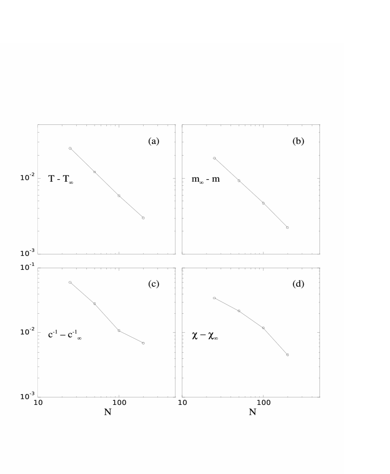
In Fig. 1 we show the results for the energy density . The simulation time is . The figure contains four plots in log-log scale, in which we show, as a function of the number of particles, the difference between the average value of four observables obtained in the finite simulations and their corresponding limit computed through the large deviation method (indicated by the subscript ). The four observables are: the microcanonical temperature (26), the magnetization (22), the inverse specific heat (4.1) and the magnetic susceptibility (28). Actually, for the magnetization, the plotted quantity is the limit value minus the finite value, which is smaller. Furthermore, for the inverse specific heat we have considered the intensive quantities that are obtained multiplying (4.1) and (45) by (and then we have used the lower case for the corresponding symbol).
Assuming a power law decay with of the simulated averages towards the limit value, the exponent of this law can be estimated from a fit with a straight line. In the plots the lines are interpolations between points, as a guide to the eye. We do not show the fitting lines that can be easily obtained. We limit to point out that the slope of these lines is in all cases close to . This behavior should be expected on general grounds; in fact, the finite corrections could be obtained by the successive terms in the saddle point evaluation related to the large deviation computation, and the first correction is expected in general to scale like .
6 Conclusions and perspectives
In this paper we have considered in parallel two methods for the evaluation of microcanonical averages of macroscopic observables and we have applied them to the mean-field model in an external magnetic field.
We have implemented in the model the general expressions that, through the microcanonical formalism introduced by Rugh [17, 18], allow us to compute an entire set of macroscopic quantities (temperature, magnetization, specific heat, magnetic susceptibility, etc.), performing time averages of suitable mechanical observables at finite . In particular, these macroscopic variables are obtained taking derivatives of the entropy with respect to the energy density and to other parameters of the Hamiltonian, like the external field (see e.g. formulas (4.2)).
Then, we have considered large deviation techniques, whose applicability relies on the determination of a set of macroscopic variables on which the energy depends in a simple way. This is generally possible for systems with long-range interactions, although the method is viable also for other cases [19]. Our model, being of the mean-field type, can be solved exactly in the microcanonical ensemble, using large deviation techniques. This leads to the analytic determination of the same macroscopic quantities in the thermodynamic limit.
The purpose was here to derive the actual expressions of macroscopic observables that stem from the application of the two different methods mentioned above to a model that has already been a subject of study for its interesting dynamical properties [21, 22]. Although these two approaches lead to expressions which show no evident similarity, especially for specific heat and magnetic susceptibility, the time averages computed with Rugh’s microcanonical formalism converge to the thermodynamic limit value computed with large deviations. Corrections are of order .
We find that the specific heat and the magnetic susceptibility converge extremely slowly in time, unless one devises methods to “help” the system explore more efficiently phase space. The method we use consists in periodically reshuffling particle velocities. These observables, which correspond to higher order derivatives of the entropy, have extremely complex expressions, and this could be at the origin of the observation of such slow convergence. However, we believe that this slow relaxation is rather a distinctive signature of the long-range (mean-field) nature of the model. Indeed, slow time relaxations are quite common in such systems and have been already observed in other models [2, 22, 24, 25], being associated to the presence of the so-called quasi-stationary states.
In a future paper [16] we will concentrate on the properties of this model in the low energy/temperature phase. We will show the presence of ensemble inequivalence features and of a negative susceptibility in the microcanonical ensemble.
While finishing this paper we became aware of a very recent study of the model without external field which uses large deviation techniques [23]. However, this work focuses on different aspects, being devoted to a detailed study of the non-analiticity properties of the entropy function.
References
- [1] D. H. E. Gross, Microcanonical Thermodynamics: Phase Transitions in Small Systems, Lecture Note in Physics, 66, World Scientific, Singapore, 2001.
- [2] T. Dauxois, S. Ruffo, E. Arimondo, M. Wilkens (Eds.), Dynamics and Thermodynamics of Systems with Long-Range Interactions, Lecture Notes in Physics 602, Springer-Verlag, New York, 2002.
- [3] F. Gulminelli, Ph. Chomaz, Phys. Rev. E 66 (2002) 046108.
- [4] P. Hertel, W. Thirring, Ann. Phys. 63 (1971) 520.
- [5] M. K. H. Kiessling, J. L. Lebowitz, Lett. Math. Phys. 42 (1997) 43.
- [6] R. S. Ellis, K. Haven, B. Turkington, J. Stat. Phys. 101(2000) 999.
- [7] R. S. Ellis, Entropy, Large Deviations, and Statistical Mechanics, Springer, New York, 1985.
- [8] J. Barré, D. Mukamel, S. Ruffo, Phys. Rev. Lett. 87 (2001) 030601.
- [9] R. S. Ellis, H. Touchette, B. Turkington, Physica A 335 (2004) 518.
- [10] R. S. Ellis, P. Otto, H. Touchette, cond-mat/0409047 (2004), to be published in Ann. Appl. Prob.
- [11] M. Costeniuc, R. S. Ellis, H. Touchette, J. Math. Phys. 46 (2005) 063301.
- [12] D. Lynden-Bell, Physica A 263 (1999) 293.
- [13] V. A. Antonov, Leningrad Univ. 7 (1962) 135; Translation in IAU Symposium 113 (1995) 525; D. Lynden-Bell, R. Wood, Monthly Notices of the Royal Astronomical Society 138 (1968) 495.
- [14] M. Schmidt et al., Phys. Rev. Lett. 86 (2001) 1191.
- [15] F. Gobet et al., Phys. Rev. Lett. 87 (2001) 203401.
- [16] A. Campa, S. Ruffo, H. Touchette, in preparation.
- [17] H. H. Rugh, J. Phys. A: Math. Gen. 31 (1998) 7761.
- [18] H. H. Rugh, Phys. Rev. E 64 (2001) 055101.
- [19] R. S. Ellis, Physica D 133 (1999) 106.
- [20] J. Barré, F. Bouchet, T. Dauxois, S. Ruffo, J. Stat. Phys. 119 (2005) 677.
- [21] R. C. Desai, R. Zwanzig, J. Stat. Phys. 19 (1978) 1.
- [22] T. Dauxois, S. Lepri, S. Ruffo, Comm. Nonlinear Sc. Num. Simul. 8 (2003) 375.
- [23] I. Hahn, M. Kastner, cond-mat/0506649 (2005).
- [24] Y. Y. Yamaguchi, J Barré, F. Bouchet, T. Dauxois, S. Ruffo, Physica A, 337 (2004) 36.
- [25] H. Morita and K. Kaneko, cond-mat/0506261.