Coherent regimes of mutually coupled Chua’s circuits

Abstract

We study the dynamical regimes that emerge from the strongly coupling between two Chua’s circuits with parameters mismatch. For the region around the perfect synchronous state we show how to combine parameter diversity and coupling in order to robustly and precisely target a desired regime. This target process allows us to obtain regimes that may lie outside parameter ranges accessible for any isolated circuit. The results are obtained by following a recently developed theoretical technique, the order parameter expansion , and are verified both by numerical simulations and on electronic circuits. The theoretical results indicate that the same predictable change in the collective dynamics can be obtained for large populations of strongly coupled circuits with parameter mismatches.

I Introduction

One of the most important features of interacting oscillating units is the possibility for their motions to entrain each other and evolve in synchronicity. The phenomenon of synchronization is a universal feature underlying the collective behavior of populations of dynamical systems and its importance has been recognized in many different fields Pikovsky and Maistrenko (2003); Mosekilde et al. (2002); Manrubia et al. (2004). In particular, a great deal of attention has been devoted to globally-coupled dynamical systems as a model for a variety of physical Oliva and Strogatz (2001), chemical Kuramoto (1984); Kiss et al. (2002a) and biological systems Danø et al. (1999); Winfree (2001).

Contrary to the assumption of identical units, common in many theoretical approaches, real systems display an unavoidable diversity in the oscillator population showing up as, e.g., parameter mismatches. The effect of such a diversity might hinder synchronization and yields an incoherent regime if the coupling is too weak. The main feature of incoherence is that the motions of the individual systems are largely independent to each others. The collective dynamics, then, is either stationary in average (for infinite number of elements) or displays fluctuations that scale with the population size. When the coupling strength is increased, some or all the elements of the population synchronize and, as a result, oscillations start to be detected at a macroscopic level. The transition to collective oscillations is typically accompanied by rather complex regimes, such as clustering Osipov and Sushik (1998), partial synchronization Matthews et al. (1991), phase synchronization Rosenblum et al. (1996), etc. For even stronger coupling, complete synchronous regimes, characterized by a high degree of coherency within the population, develops. This means that all the population elements share the same kind of dynamics, apart from small differences due to the microscopic diversity, and this dynamics reflects at the macroscopic level.

Despite of the numerous theoretical advances in the analysis of globally coupled dynamical systems, the experimental verification has revealed to be extremely difficult, in particular as far as biological systems are concerned. The Kuramoto transition from incoherence to the locked state is in this sense a good example Kuramoto (1975). It dates back to 1975 and is one of the best known and general results in synchronization theory. However, to our best knowledge, it has been quantitatively verified once in experiments and required the implementation of an ad hoc system Kiss et al. (2002b). Two main problems are encountered in experiments. One is the difficulty in controlling or measuring the parameter variability in the system. The second one is related to the global coupling which is very rare in nature. These experimental limitations are especially relevant for regimes close to the incoherence one where a large population is needed.

In order to avoid these problems associated with incoherence, in this paper we focus instead on globally coupled systems close to the synchronous state. As it was recently shown, such coherent states do not strongly depend on the population size De Monte and d’Ovidio (2002); De Monte et al. (2003). This fact is very interesting from the experimental viewpoint because the main characteristics can be studied in systems of only two elements and the results extended to larger populations. Moreover, the coherent dynamics may be described by a set of low dimensional equations with only few parameters. Transitions among different regimes correspond to bifurcations involving a small number of dimensions and parameters, thus having the advantage of being very robust to changes in the microscopic features of the population.

As an application of such theoretical results, we study the strong coupling regimes of two Chua’s circuits. Chua’s circuits offer an intermediate step between theory and applications. They can be modelled with a simple set of non-linear equations, thus allowing the use of analytical methods and quick numerical simulations. At the same time they can be easily implemented in hardware. Even if they constitute a rather controlled experimental system, a verification of theoretical results faces a test on its robustness with respect to: (i) noise fluctuations in states and parameter values, (ii) constrains in the accessible parameter precision and ranges, and (iii) small functional mismatches between model and implementation. Finally, Chua’s circuits are particularly interesting because they constitute prototypical devices for nonlinear system testbeds.

Section II derives the equations for the macroscopic dynamics of an interacting population (of any size) in the coherent regime. This representation allows us to infer on the dynamical regimes of the experimental system. We then provide two examples of comparison between theoretical prediction and experimental system. In Sec. III we show how, by controlling parameter mismatch, one can drive the mean field to regimes that are different from the uncoupled dynamics and that might not be accessible by any of the individual systems. In Sec. IV we consider the case in which the individual elements differ for the time scale of their motion, and focus in particular on the regime of oscillaton death, where parameter diversity induces a suppression of the individual and collective oscillations. Finally, Sec. V is devoted to the discussion of the results and to their possible applications.

II Order parameter expansion of mutually coupled Chua’s circuits

The order parameter expansion De Monte and d’Ovidio (2002); De Monte et al. (2003) is a useful technique for studying regimes that bifurcate from the perfectly synchronous state in populations of globally and strongly coupled elements when the parameter mismatch is increased. Let us here review the main results by considering a system of the form:

$$\dot{x_{j}}=f\left(x_{j},p_{j}\right)+K(X-x_{j})\hskip 28.45274ptj=1,2,\dots,N.$$ (1)

where $p_{j}$ is a parameter containing the diversity of the system and the dynamics of the each element $f_{j}(x_{j})=f\left(x_{j},p_{j}\right)$, is defined by the smooth function $f_{j}:\mathbb{R}^{n}\rightarrow\mathbb{R}^{n}$. All the elements are coupled to the the mean field of the population $X=\langle x_{j}\rangle$ through the coupling function $K(X-x_{j})$ that, as we will see later, for the case of the electronic coupling we use, can be assumed as a linear diagonal operator (in fact, a more general system can be considered, see De Monte et al. (2004) for details.) The basic idea of the method is to obtain an effective equation of motion for the mean field variable $X$, valid when all the elements evolve in time close to $X$. This is done by considering regimes close to the perfectly synchronous state, defined as $x_{j}=X,\,\forall j$. Under this assumption, equation (1) can be expanded into the individual deviations from the mean field $\epsilon_{j}=x_{j}-X$ and from the mean parameter $\delta_{j}=p_{j}-p_{0}$, being $p_{0}=\langle p\rangle$. By averaging Eq. (1) over the population, one gets, at first order, the following approximated equation for the mean field:

$$\begin{cases}\dot{X}=F(X,p_{0})+D_{x,p}F(X,p_{0})\,W\\ \\ \dot{W}=\sigma^{2}\,D_{p}\,F(X,p_{0})+(D_{x}\,F(X,p_{0})-K)\,W,\end{cases}$$ (2)

where $W=\langle\delta\,\epsilon\rangle$ is a second macroscopic variable, or shape order parameter; $p_{0}$ is the average parameter value and $\sigma^{2}$ is the standard deviation of the parameter distribution. Besides being low dimensional, such equation has the advantage of having a clear physical meaning: the mean field behaves like the average element, perturbed by a macroscopic variable that quantifies the mismatch in phase and parameter space. The macroscopic regimes thus appear as an unfolding of the perfectly locked state $\dot{X}=F(X,p_{0})$ and are controlled by the parameter $K$ and $\sigma^{2}$. Such equation holds when the displacements from the mean field $\epsilon_{j}$ are small, and thus, operationally, when the coupling is sufficiently strong compared with the parameter mismatch. Another important consideration is that Eq. (2) does not depend on the population size. Consequently, the results we obtain for two Chua’s circuits can be readily generalized to larger arrays.

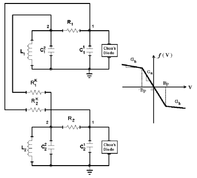
Figure 1: Scheme of the two mutually coupled Chua’s circuits. The parameters are $C_{1,2}^{1}=10.2$ nF ,$C_{1,2}^{2}=101.8$ nF, $L_{1,2}=18.4$ mH, $R_{1,2}=1562$ Ohm, $G_{1,2}^{a}=-7.625\,10^{-4}$, $G_{1,2}^{b}=4.12\,10^{-4}$.

Let us now apply Eq. (2) to the case of two mutually coupled Chua’s circuits. The configuration of the circuits that we study is shown in Fig. 1. The equations are easily written in terms of the voltages $v_{1}$ and $v_{2}$ (at point 1 and 2 respectively) and the current $I$ at point 3, the first circuit is described by:

$$\begin{cases}\dot{v}_{1}^{1}=&\frac{1}{C_{1}^{1}R_{1}}\,v_{1}^{2}-\frac{G_{1}^{a}-G_{1}^{b}}{2C_{1}^{1}}\left(|v_{1}^{1}+B_{1}^{p}|-|v_{1}^{1}-B_{1}^{p}|\right)\\ \rule[-17.07164pt]{0.0pt}{31.29802pt}&-\frac{1}{C_{1}^{1}}\left(G_{1}^{b}+\frac{1}{R_{1}}\right)v_{1}^{1}+\frac{1}{C_{1}^{1}R^{k}_{1}}\,(v_{1}^{1}-v_{2}^{1}\\ \rule[-17.07164pt]{0.0pt}{22.76219pt}\dot{v}_{1}^{2}=&\frac{1}{C_{1}^{2}}\,I^{1}+\frac{1}{C_{1}^{2}R_{1}}\left(v_{1}^{1}-v_{1}^{2}\right)+\frac{1}{C_{1}^{2}R^{k}_{2}}\,(v_{1}^{2}-v_{2}^{2})\\ \rule[-8.53581pt]{0.0pt}{22.76219pt}\dot{I}_{1}=&-\frac{r_{1}^{b}}{L_{1}}\,I_{1}-\frac{1}{L_{1}}\,v_{1}^{2}\end{cases}$$ (3)

where $R^{1,2}_{k}$ are the two coupling resistors. These resistors will be used as control parameters. Other internal parameters, that are kept constant, are displayed in the caption of Fig. 1. The second circuit has an equivalent equation, with lower index 2 instead. Before proceeding with the analysis, it is worth mentioning that the mutual coupling Eq. (3) term can be recast in the form of a global coupling term, so that the correspondence with Eq. (2) is readily established. The dependence on the mean field becomes apparent by noticing that:

$$\left(v_{2}^{1}-v_{1}^{1}\right)=\left(v_{2}^{1}+v_{1}^{1}-2v_{1}^{1}\right)=2\left(\langle v_{1}\rangle-v_{1}^{1}\right).$$ (4)

The coupling constants are the multiplicative factors $1/(C^{1}R^{1}_{k})$ and $1/(C^{2}R^{2}_{k})$. At this point, we recover Eq. (1) by identifying $x_{j}$ with the vector ${<v_{j}^{1},\,v_{j}^{2},\,I_{j}>}$ and $f_{j}(x_{j})$ with the equation for an uncoupled Chua circuit. The coupling matrix is:

$$K^{1}=\left[\begin{matrix}\frac{1}{C_{1}^{1}R^{1}_{k}}&0&0\\ 0&\frac{1}{C_{1}^{2}R^{2}_{k}}&0\\ 0&0&0\end{matrix}\right]$$ (5)

Since we assume identical capacities for the two circuits, the coupling is symmetrical. The explicit calculation of the reduced equations are given in the Appendix. With this formalism, we are now ready to use Eq. (2) on some specific condition and to study the collective regimes that emerge due to the interplay of parameter mismatch and coupling.

III Strong mutual coupling

Let us first address the case in which the mismatch is in the internal resistors $R_{1,2}$ of the two circuits, while the other internal parameters are kept identical. The coupling resistors $R_{k}^{1,2}$ are chosen weak enough to ensure that the coupling is strong and the regime coherent. Under such strong coupling conditions, the collective dynamics will be qualitatively equal to the dynamics of an “average oscillator”. This corresponds to a system of equations identical to those of each single element, except for the parameter on which diversity is imposed, that is instead substituted by its average value. Intuitively, such property of the macroscopic dynamics is due to the fact, that when the coupling matrix is predominantly diagonal, the shape parameter $W$ is kept small. This corresponds to the situation in which the population is tightly packed around the mean field. In the limit in which the coupling is infinitely strong, $W$ vanishes and in Eq. (2) we end up with the equation for an average oscillator.

Such a consideration has interesting implications in the control of the collective behavior of populations of dynamical systems, as well as in the detection of the microscopic features in terms of purely macroscopic observations. Indeed, the dynamics that is stabilized by coupling non-identical circuits may not be attainable by any of them if uncoupled. The collective regime is thus “coded” in the diversity and coupling rather than in the internal features of the individual circuits. Moreover, Eq. (2) allows a straightforward identification of such a hidden collective behavior.

As a first application of the aforementioned theoretical results, let us examine the case when both circuits operate in a periodic regime. Figure 2 (a) and (b) displays the experimentally measured attractors of the two uncoupled circuits, of period 3 and 4 respectively. Figure 2 (c) and (d) show that, as a result of the coupling, both oscillators behave chaotically, although the mismatch in the parameters has only minor effects on their individual dynamics.

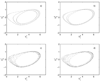
Figure 2: Collective chaotic behavior as generated by coupling two nonidentical circuits, each of which is individually periodic. a) and b) Uncoupled chaotic dynamics of the two circuits ($R_{1}=1740$ Ohm, $R_{2}=1644$ Ohm). c) Attractor of the first circuit after the coupling is established. Being the coupling strong ($R_{k}^{1,2}=200$ Ohm), the attractors of the second circuit and of the mean field are nearly identical to this one and thus are not shown. d) The same behavior of the strongly coupled circuits is predicted by a single circuit with the internal resistance set at $(R_{1}+R_{2})/2=1692$ Ohm.

The same idea can be used for stabilizing unstable periodic orbits. Let us, for instance, consider the case in which both circuits are chaotic, but their parameter values are located, when the circuits are uncoupled, on the opposite side of a periodic window. Figure 3 shows that once they are coupled, both circuits get synchronized onto a period-three orbit. The coupling thus results into the stabilization of an unstable orbit embedded into the chaotic attractor.

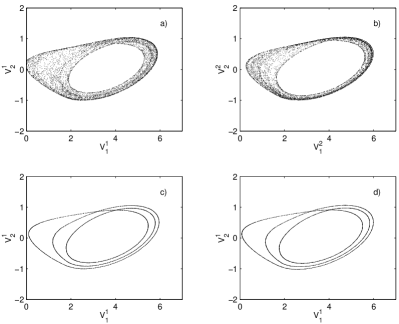
Figure 3: Stabilization of an unstable period-three orbit by coupling of two nonidentical chaotic circuits. a) and b) Uncoupled chaotic dynamics of the two circuits ($R_{1}=1621,\,R_{2}=1745$ Ohm). c) Attractor of the first circuit after the coupling is established. Being the coupling strong, the attractors of the second circuit and of the mean field are nearly identical to this one and thus are not shown. d) As in the Fig.2 the dynamics of the coupled circuits can be predicted by a single circuit with the internal resistance at the average value $(R_{1}+R_{2})/2=1683$ Ohm.

The possibility of obtaining a qualitatively novel dynamics by coupling two circuits with different internal parameters is robust with respect to changes in the coupling intensity (also under differential modifications of the resistors) as long as both coupling resistors are sufficiently weak, that is coupling is sufficiently strong. This robustness was confirmed by repeating the two experiments described above for several values of the coupling resistors.

Besides providing a way for targeting specific regimes, the experiments also show that the mathematical limit of infinitely strong coupling is actually attainable, to a good approximation, even for experimental feasible resistance values. It is also important to remark that in order to target a regime one only needs to know the bifurcation diagram: this information can be obtained experimentally and in principle does not require the knowledge of the functional form of $f$.

IV Oscillation death in circuits with time scale mismatch

In this section we address oscillaton death, a regime where the dynamics of each population element is suppressed as a collective effect, i.e., resulting from the interplay of coupling and diversity. Oscillator death has been firstly described in populations of limit cycle oscillators with direct Ermentrout and Troy (1989); Ermentrout (1990) or time-delayed coupling Atay (2003). Recently, an order parameter expansion has been used to demonstrate that this regime may arise under generic conditions in populations of globally coupled element with time scale mismatch De Monte et al. (2003). Such results introduce us to the next study on coupled circuits. The equations for a population with time scale mismatch and global, linear coupling can be written as:

$$\dot{x_{j}}=\tau_{j}f\left(x_{j}\right)+K(X-x_{j}),\hskip 28.45274ptj=1,2,\dots,N.$$ (6)

This equation may be seen as a simple way for generalizing the Kuramoto model, where the distributed parameter is the natural frequency of the oscillators, to an individual dynamics different from a limit cycle. The peculiar parameter dependence of Eq. (6) is reflected in a simple form of the reduced system:

$$\begin{cases}\dot{X}=\langle\tau\rangle f(X)+J\,W\\ \\ \dot{W}=\sigma^{2}\,f(X)+(\langle\tau\rangle J-K)\,W,\end{cases}$$ (7)

where $J$ is the Jacobian $D_{x}f(x)$.

Due to the multiplicative nature of the distributed parameter in Eq. (6), any fixed point of $f$ is also a fixed point for the mean field. The stability of such a point, however, can change due the presence of the coupling and time scale mismatch. With some algebra one finds that generic conditions exist under which an unstable focus of $f$ becomes attracting for the population. Referring to De Monte et al. (2003) for the details, here we just notice that, if the time scale mismatch is sufficiently wide, this equilibrium is stabilized for “intermediate” values (i.e., large enough to avoid incoherence and smaller than those where nonstationary coherent solutions are present) of the coupling.

For the case of Chua circuits, one can see from Eq. (3) that the time scale can be easily changed by tuning the capacitors $C_{1}$, $C_{2}$ and the inductance $L$. We modify the time scale of one of the two circuits by making use of commercially available capacitors and inductances, thus obtaining a mismatch of at most 14%. Both circuits, when uncoupled, have similar chaotic dynamics (double scroll attractor) although their time evolution takes place with different speed.

The bifurcation diagram of the reduced system Eq. (7) can be numerically computed for an interval of time scale differences comparable to that accessible in our experimental setup. The diagram provides the coherent regimes of diffusively coupled Chua circuits as a function of their parameter diversity and is indipendent of the population size. As expected from the previous section, for a low value of the coupling resistors (strong coupling), the circuits are entrained on a chaotic attractor indistinguishable from the uncoupled dynamics. However, when the coupling is reduced a cascade of coherent regimes bifurcates from the chaotic attractor and eventually the state of oscillator death is reached (Fig. 4).

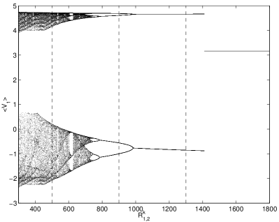
Figure 4: Bifurcation diagram of the reduced system Eq. (7). The Poincaré section of the attractor is shown as a function of the parameter mismatch between the two circuits, indicating that an increase in diversity induces a transition from a two-lobes to a one-lobe attractor. This macroscopic attractor then undergoes a backward period-doubling bifurcation cascade to a limit cycle, and eventually a fixed point is stabilized through a subcritical bifurcation.

The resistances $R^{1}_{k}=R^{2}_{k}=R_{k}$ of the coupled circuits can now be tuned in order to target a specific collective regime, according to the numerical characterization of the reduced system. Figure 5 shows some of the emergent dynamics experimentally observed. The oscillation death regime also appears in the circuits for $R^{k}$ slightly above $1.5$ k$\Omega$ (not shown).

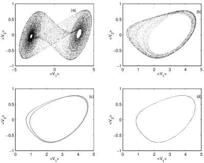
Figure 5: Experimental behaviour of the coupled circuits at maximum coupling $R_{k}=0$ (a) and at values indicated in the bifurcation diagram of the reduced system Fig. 4 (b-d).

V Conclusions

Although the importance of emergent behavior in populations of nonidentical dynamical systems is widely recognized, only few experimental systems offer the necessary degree of control for testing the theoretical results. Here, we have proposed the implementation of a circuit aimed at mimicking the coherent behavior of populations with parameter mismatch in the region of strong coupling. Theoretical results and numerical simulations suggest that this case is representative of larger populations and constitute a tool for addressing diversity-dependent coherent dynamics.

The experimental system was composed of two symmetrically coupled Chua circuits, the diversity in their components introduces a mismatch in the internal parameters. We have shown that the average dynamics of such coupled systems can be very different from that of the individual circuits when decoupled. The order parameter expansion developed for populations of strongly coupled dynamical systems allowed us to predict such a collective behavior based on the knowledge of the uncoupled dynamics. In this way, the emergent dynamics can be tuned, by controlling the parameter mismatch, onto an attractor that might not be reachable with any of the individual circuits. The possibility of robustly targeting a specific coherent regime can find a wide applicability in populations of globally coupled non-identical systems, the chaotic behavior of Chua circuits being just one example of individual dynamics.

As a second example of diversity-induced qualitative changes of the collective behavior, we have addressed the case when the circuits differ by their time scales. In this case, the assumption that the coupling matrix is independent of the parameters is valid for sufficiently small parameter mismatch.

The coherency of the dynamics is not only the basic assumption that allows us to analytically address the collective regimes, but also guarantees that the results obtained for two circuits can be extended to populations of many elements with a comparable variance of the parameter diversity. The robustness of strong coupling regimes to changes in the number of interacting circuits is confirmed by numerical simulations. These show indeed that the collective behaviour is selected according to the parameter distribution variance rather than from the actual population size.

VI Acknowledgments

S.D.M. is thankful for the hospitality of DFI-IMEDEA and is supported by the EIF Marie-Curie fellowship 010169. The authors thank W. Korneta for interesting discussions and M. Oprandi for technical help. This work has been partly supported by MEC (Spain) and FEDER through project CONOCE2 (FIS2004-00953).

VII appendix

The equations approximating the average dynamics of a population with time scale mismatch can be computed for the Chua circuits that we have addressed in this paper starting from Eq. (3). The collective dynamics is described by a system of six equations (three for the variables of the average $X=[\langle v_{1}\rangle,\langle v_{2}\rangle,\langle cr\rangle]$ and three for the shape parameter $W$. This can be compactly written as (6), where $f(X)$ is a vector of components:

$$f(1)= -\frac{G^{b}}{C^{1}}\,v_{1}+\frac{v_{2}-v_{1}}{R\,C^{1}}-\frac{G^{a}-G^{b}}{2\,C^{1}}$$

$$\times\left(|v_{1}+B^{p}|-|v_{1}-B^{p}|\right)$$

$$f(2)= \frac{1}{C_{2}}\,\left(I+\frac{v_{1}-v_{2}}{R}\right)$$

$$f(3)= -\frac{1}{L}\,\left(I\,r^{b}-v_{2}\right).$$

The coupling matrix $\mathcal{K}$ is:

$$\mathcal{K}=\left[\begin{matrix}&\frac{2}{C_{1}\,R^{k}_{1}}&0&0\\ &0&\frac{2}{C_{2}\,R^{k}_{2}}&0\\ &0&0&0\end{matrix}\right]$$

and the Jacobian matrix $\mathcal{J}$ is:

$$\mathcal{J}=\left[\begin{matrix}&j_{1,1}&\frac{1}{C_{1}\,R}&0\\ \\ &\frac{1}{C_{2}\,R}&-\frac{1}{C_{2}\,R}&\frac{1}{C_{2}}\\ \\ &0&-\frac{1}{L}&-\frac{r_{b}}{L}\end{matrix}\right],$$

where

$$j_{1,1}= -\frac{G_{b}}{C_{1}}+\frac{1}{R\,C_{1}}+\frac{G_{a}-G_{b}}{2\,C_{1}}$$

$$\times\left[sgn(v_{1}+B_{p})-sgn(v_{1}-B_{p})\right].$$

References

- Pikovsky and Maistrenko (2003) A. Pikovsky and Y. Maistrenko, eds., Synchronization: Theory and application (Kuwler, Dordrecht/Boston/London, 2003).
- Mosekilde et al. (2002) E. Mosekilde, Y. Maistrenko, and D. Postnov, Chaotic Synchronization: Applications to Living Systems (World Scientific, Singapore, 2002).
- Manrubia et al. (2004) S. C. Manrubia, A. S. Mikhailov, and D. H. Zanette, Emergence of dynamical order: synchronization phenomena in complex systems (World Scientific, Singapore, 2004).
- Oliva and Strogatz (2001) R. A. Oliva and S. H. Strogatz, Int. J. of Bif. and Chaos 11, 2359 (2001).
- Kuramoto (1984) Y. Kuramoto, Chemical Oscillations, Waves and Turbulence (Springer, Berlin, 1984).
- Kiss et al. (2002a) I. Z. Kiss, Y. Zhai, and J. L. Hudson, Science 296, 1676 (2002a).
- Danø et al. (1999) S. Danø, P. G. Sørensen, and F. Hynne, Nature 402, 320 (1999).
- Winfree (2001) A. T. Winfree, The Geometry of Biological Time, 2nd edition (Springer, New York, 2001).
- Osipov and Sushik (1998) G. Osipov and M. Sushik, Phys. Rev. E 58, 7198 (1998).
- Matthews et al. (1991) P. C. Matthews, R. E. Mirollo, and S. H. Strogatz, Physica D 52, 293 (1991).
- Rosenblum et al. (1996) M. G. Rosenblum, A. Pikovsky, and J. Kurths, Phys. Rev. Lett. 76, 1804 (1996).
- Kuramoto (1975) Y. Kuramoto, in International Symposium on Mathematical Problems in Theoretical Physics, edited by H. Araki (Springer, New York, 1975), vol. 39 of Lecture Notes in Physics, p. 420.
- Kiss et al. (2002b) I. Z. Kiss, Y. Zhai, and J. L. Hudson, Science 296, 1676 (2002b).
- De Monte and d’Ovidio (2002) S. De Monte and F. d’Ovidio, Europhys. Lett. 58, 21 (2002).
- De Monte et al. (2003) S. De Monte, F. d’Ovidio, and E. Mosekilde, Phys. Rev. Lett. 90, 054102 (2003).
- De Monte et al. (2004) S. De Monte, F. d’Ovidio, H. Chaté, and E. Mosekide, Phys. Rev. Lett. 92, 254101 (2004).
- Ermentrout and Troy (1989) G. B. Ermentrout and W. C. Troy, SIAM J. Math. Anal. 20, 1436 (1989).
- Ermentrout (1990) G. B. Ermentrout, Physica D 41, 219 (1990).
- Atay (2003) F. Atay, Phys. Rev. Lett. 91, 094101 (2003).