Diffusion of Monochromatic Classical Waves

Abstract

We study the diffusion of monochromatic classical waves in a disordered acoustic medium by scattering theory. In order to avoid artifacts associated with mathematical point scatterers, we model the randomness by small but finite insertions. We derive expressions for the configuration-averaged energy flux, energy density, and intensity for one, two and three dimensional (1D, 2D and 3D) systems with an embedded monochromatic source using the ladder approximation to the Bethe-Salpeter equation. We study the transition from ballistic to diffusive wave propagation and obtain results for the frequency-dependence of the medium properties such as mean free path and diffusion coefficient as a function of the scattering parameters. We discover characteristic differences of the diffusion in 2D as compared to the conventional 3D case, such as an explicit dependence of the energy flux on the mean free path and quite different expressions for the effective transport velocity.

I Introduction

The ongoing interest in the field of classical waves in complex media is caused by the importance of detection and imaging techniques that are based on wave propagation and scattering. This ranges from electromagnetic waves in optical and near infrared tomography ar1 and microwave radars fu1 to acoustic waves in ultrasonics fr1 and geophysics sn1 . Complexity is often associated with inhomogeneities that cause scattering which complicates most imaging processes considerably. However, when used cleverly, the scattered field can also be used to improve imaging ld1 . Although length scales (with respect to the wavelength) and the degree of the disorder may vary considerably from field to field, methods and results have been shown to be interchangeable without much difficulty ps1 . Recent topics of interest include localization of classical waves wl1 ; hs1 , the transition from ballistic to diffusive wave propagation zj1 , acoustic time-reversal imaging mf1 , etc. Direct simulation by the exact solution of a well-known Helmholtz wave equation for a given realization of the medium is often the method of choice for given applications. The drawbacks of the brute force computational approach are the limited system size and statistics that can be achieved with given computer resources as well as the difficulty to distill general principles out from the plethora of output data. The need for simple models with transparent results therefore remains.

An analytic theory of wave propagation in disordered media necessarily relies on simple model scatterers, for which point scatterers, i.e. (regularized) $\delta$-functions in real space, are often chosen vc1 ; rn1 . Unfortunately, the scattering response of a single point scatterer can become non-causal, a pathological behavior that can not be solved by a simple momentum cutoff bf1 . Especially for the study of the frequency dependence over a wider range it is therefore necessary to use more realistic model scatterers.

In this paper we wish to study a simple but not unrealistic experiment for the determination of the scattering properties of scalar waves in a disordered bulk material. A signal is emitted by a source and detected by a receiver, both embedded in the medium at sufficiently large distances from the boundaries. Ultimately, we are interested in the detector signal caused by a pulsed (broadband) signal emitted by the source. After a first arrival we then expect the so-called coda that arrives at later times due to multiple scattering at the random scatterers sf1 . However, combining both the effects of multiple scattering and the full frequency dependence of the scattering processes renders an analytical treatment difficult without additional approximations, such as a complete neglect of the frequency dependence of the scattering amplitudes tf1 . In order to understand how to justify certain approximations and eventually find better ones, we have carried out a study of the frequency dependence of the scattering properties of random media. We concentrate on the steady state in the presence of strictly monochromatic sources, which distinguishes the present work from related studies of the propagation of narrow band pulses lt1 . As main results we obtain the frequency dependence of macroscopic effective medium properties like the mean free path and the diffusion constant that depend on the microscopic parameters of the random scatterers.

When the ratio between source-receiver distance and mean free path is small, wave propagation is predominantly ballistic. When this ratio is large, energy and intensity propagation is governed by the diffusion equation rn1 ; tf1 . Both these regimes are well understood. However, many imaging applications operate on length scales where the mean free path and the source-receiver distance are comparable. This is especially the case in geophysics where mean free paths range from a few hundred meters up to tens of kilometers ht1 . The behavior at this crossover regime between ballistic and diffuse wave (intensity) propagation is of considerable interest zj1 and also subject of the present study.

Here we present an analytical formalism on monochromatic wave intensity and energy propagation in one dimensional, two dimensional and three dimensional (1D, 2D and 3D) homogeneously disordered media using realistic model scatterers. We determine the relative contributions of diffusively and coherently propagated waves as the source-receiver distance increases. We did no find many theoretical studies of wave propagation in two dimensional random media in the literature ps1 ; td1 , although several experiments on quasi 2D systems have been carried out tf1 ; st1 . Another possible test for our 2D theory is comparison with numerical studies, which for very large systems are much cheaper than in the 3D case.

The remainder of this paper is organized as follows. In sections II-IV we start with defining our model system and the basic equations, addressing the scattering matrices of single scatterers and discussing the average amplitude propagators in the frequency domain. The intensity, energy flux and energy density are discussed in section V. Results on the frequency dependence of the diffusion constant and its dependence on the model parameters are discussed in section VI. In general, the results for 1D systems are easily obtained, whereas our results for 3D systems agree with findings previously reported by others. The mathematics in the 2D case is not trivial, however, and the derivations are summarized in the appendix. We end with the conclusions.

II Definitions and basic equations

II.1 Microscopic equations

We describe the propagation of (scalar) acoustic waves in a microscopic model system. Specifically, we consider a 1D, 2D or 3D acoustic medium with wave velocity $c_{0}$ and a mass density $\rho_{0}$. The medium contains $n$ randomly distributed scatterers per unit length, area or volume and we treat the dilute limit in which the average distance between scatterers is much larger than their radius $a$. The internal wave velocity of a scatterer is $c_{int}$ and, for simplicity, the difference in mass density with the surrounding medium is disregarded. The waves are emitted by a monochromatic point source oscillating at frequency $\omega$ positioned at the origin. The wave amplitude $\psi_{\omega}$, related to the hydrostatic pressure by $p_{\omega}=\partial_{t}\psi_{\omega}$ and to local particle velocity by $v_{\omega}=-\rho_{0}^{-1}\nabla\psi_{\omega}$, then obeys the wave equation:

$$\left(\mathbf{\nabla}^{2}+c^{-2}\left(\mathbf{r}\right)\partial_{t}^{2}\right)\psi_{\omega}\left(\mathbf{r};t\right)=-Q\rho_{0}\delta\left(\mathbf{r}\right)\cos\left(\omega t\right)\text{.}$$ (1)

The source term chosen here corresponds to a volume injection term. The source emits plane waves for 1D, cylindrical waves for 2D and spherical waves for 3D media. In all cases $Q$ is in units of length per unit time. The wave velocity profile of the entire medium $c\left(\mathbf{r}\right)$ contains the information of the positions of the scatterers (in 1D $\mathbf{r}=x$).

The Green function of the Helmholtz equation (1) in the real space and frequency domain reads

$$\left[\mathbf{\nabla}^{2}+\kappa_{0}^{2}-V\left(\mathbf{r};\omega\right)\right]G\left(\mathbf{r},\mathbf{r}^{\prime};\omega\right)=\delta\left(\mathbf{r-r}^{\prime}\right)\text{,}$$ (2)

where $\kappa_{0}=\omega/c_{0}$, the length of the wave vector in the homogeneous medium. $V\left(\mathbf{r};\omega\right)$ is the scattering or impurity potential, a sum over all individual scattering potentials:

$$V\left(\mathbf{r};\omega\right)=\kappa_{0}^{2}\left(1-\gamma^{-2}\right){\displaystyle\sum\limits_{i=1}^{N}}\Theta\left(a-\left|\mathbf{r}-\mathbf{r}_{i}\right|\right)\text{.}$$ (3)

$\Theta$ is the Heaviside step function, with $\Theta\left(x\right)=0$ when $x<0$ and $1$ otherwise. The velocity contrast is defined as $\gamma=c_{int}/c_{0}$ so that the single scatterer potential is “attractive” when $\gamma<1$ and “repulsive” when $\gamma>1$. Eq. (3) describes a spherical potential, but the precise shape is not relevant when the scatterers are sufficiently small compared to the wave length.

The amplitude of the wave field is related to the Green function as

$$\psi_{\omega}\left(\mathbf{r};t\right)=-Q\rho_{0}\operatorname{Re}\left\{e^{-i\omega t}G\left(\mathbf{r},\mathbf{r}^{\prime}=0;\omega\right)\right\}\text{.}$$ (4)

The intensity $I_{\omega}\left(\mathbf{r};t\right)$ is the square of this expression. Related physical properties are the energy flux:

$$\mathbf{F}_{\omega}\left(\mathbf{r};t\right)=-\frac{1}{\rho_{0}}\partial_{t}\psi_{\omega}\left(\mathbf{r};t\right)\mathbf{\nabla}\psi_{\omega}\left(\mathbf{r};t\right)\text{,}$$ (5)

and the energy density:

$$W_{\omega}\left(\mathbf{r};t\right)=\frac{1}{2\rho_{0}}\left(\left(\mathbf{\nabla}\psi_{\omega}\left(\mathbf{r};t\right)\right)^{2}+c^{-2}\left(\mathbf{r}\right)\left(\partial_{t}\psi_{\omega}\left(\mathbf{r};t\right)\right)^{2}\right)\text{,}$$ (6)

recognized as the sum of the potential and kinetic energy contributions, respectively. For a monochromatic source with frequency $\omega$ these observables contain a time independent contribution and a second term oscillating with frequency $2\omega$. We concentrate on the constant part by time-averaging over one period. Expressed in terms of the Green function this yields

$$I_{\omega}\left(\mathbf{r}\right)=\frac{Q^{2}\rho_{0}^{2}}{2}\left|G\left(\mathbf{r},\mathbf{r}^{\prime}=0;\omega\right)\right|^{2}\text{,}$$ (7)

$$\mathbf{F}_{\omega}\left(\mathbf{r}\right)=-\frac{Q^{2}\rho_{0}\omega}{2}\operatorname{Im}\left\{G\left(\mathbf{r},\mathbf{r}^{\prime}=0;\omega\right)\mathbf{\nabla}G^{\ast}\left(\mathbf{r},\mathbf{r}^{\prime}=0;\omega\right)\right\}\text{,}$$ (8)

$$W_{\omega}\left(\mathbf{r}\right) =\frac{Q^{2}\rho_{0}}{4}\left(\left|\mathbf{\nabla}G\left(\mathbf{r},\mathbf{r}^{\prime}=0;\omega\right)\right|^{2}\right.$$

$$\text{ \ \ \ \ \ \ \ \ \ \ \ \ }+\frac{\omega^{2}}{c^{2}\left(\mathbf{r}\right)}\left.\left|G\left(\mathbf{r},\mathbf{r}^{\prime}=0;\omega\right)\right|^{2}\right)\text{.}$$ (9)

II.2 Macroscopic equations

The properties of the wave field depend via the Green function on the exact configuration of scatterers. However, in large systems, different realizations of the ensemble give similar responses (ergodicity). The similarities in the response can be studied by calculating the configurational average. This average is the connection between the microscopic description and the macroscopic (effective) medium properties.

The macroscopic (diffusively scattered) intensity of pulsed sources is usually described by the diffusion equation:

$$\partial_{t}\left\langle I\left(\mathbf{r};t\right)\right\rangle=D\nabla^{2}\left\langle I\left(\mathbf{r};t\right)\right\rangle\text{,}$$ (10)

where the brackets denote the configuration average and $D$ is the diffusion constant. In spite of neglecting the frequency dependence of the scattering processes, this approximation is known to work well in certain cases (under the condition that the source receiver distance is much larger than the mean free path) rn1 ; tf1 .

In order to obtain the steady-state diffuse intensity of a monochromatic wave field, the diffusion equation (10) is not sufficient. The energy density (and not the intensity) of the wave field is the conserved property. Eq. (10) is therefore only valid if the intensity is strictly proportional to the energy density. In general, the averaged energy transport is governed by Fick’s first law:

$$\left\langle\mathbf{F}_{\omega}\left(\mathbf{r}\right)\right\rangle=-D\left(\omega\right)\nabla\left\langle W_{\omega}\left(\mathbf{r}\right)\right\rangle\text{,}$$ (11)

accounting for the frequency dependence of the diffusion constant. In the steady-state problem and outside the monochromatic source the proper Laplace equation is

$$\nabla^{2}\left\langle W_{\omega}\left(\mathbf{r}\right)\right\rangle=0\text{.}$$ (12)

III Scattering matrices

Here we discuss the properties of a single model scatterer in the system ($N=1$ in equation (3)). The response of a system containing a monochromatic source (in the origin), a receiver (at $\mathbf{r}$) and a single “s-wave” scatterer (at $\mathbf{r}_{i}$) can be expressed in terms of Green functions of the homogeneous system ($V=0$) am1 :

$$G\left(\mathbf{r},\mathbf{r}^{\prime}=0;\omega\right) =G_{0}\left(r;\omega\right)$$

$$+G_{0}\left(\left|\mathbf{r}-\mathbf{r}_{i}\right|;\omega\right)t_{0}\left(\omega\right)G_{0}\left(r;\omega\right)\text{.}$$ (13)

This expression is valid in the far field limit ($r,r_{i}\gg\lambda$) and when scattering is isotropic ($\lambda\gg a$), where $\lambda$ is the wavelength.

The transition (t-) matrix elements for s-wave scattering are related to the scattering matrix elements by

$$t_{0}\left(\omega\right)=\left\{\begin{array}[c]{c}2i\kappa_{0}R\left(\omega\right)\text{ \ \ \ \ \ \ \ \ \ \ \ \ \ \ \ (1D)}\\ 2i\left(S_{0}\left(\omega\right)-1\right)\text{ \ \ \ \ \ \ \ \ \ (2D)}\\ 2\pi i\kappa_{0}^{-1}\left(S_{0}\left(\omega\right)-1\right)\text{ \ \ (3D)}\end{array}\right.\text{.}$$ (14)

In 1D, the s-wave scattering condition corresponds to equivalence of $t_{0}$ for either reflection or transmission. $R\left(\omega\right)$ is the reflection coefficient at a step discontinuity, it can be obtained by imposing flux conservation across the scatterer boundary. This gives em1

$$R\left(\omega\right)=e^{-i\kappa_{0}2a}\frac{R_{0}\left(1-e^{i\kappa_{0}4a/\gamma}\right)}{1-R_{0}^{2}e^{i\kappa_{0}4a/\gamma}}\text{,}$$ (15)

where $R_{0}=\left(\gamma-1\right)/\left(\gamma+1\right)$. In the same way we can derive an expression for the scattering matrix element of the s-wave channel $S_{0}$ (related to the scattering phase shift $\delta_{0}$ by $S_{0}=\exp\left(i2\delta_{0}\right)$). In 2D es1

$$S_{0}\left(\omega\right)$$

$$=-\frac{\gamma J_{0}\left(\kappa_{0}a/\gamma\right)H_{1}^{\left(2\right)}\left(\kappa_{0}a\right)-J_{1}\left(\kappa_{0}a/\gamma\right)H_{0}^{\left(2\right)}\left(\kappa_{0}a\right)}{\gamma J_{0}\left(\kappa_{0}a/\gamma\right)H_{1}^{\left(1\right)}\left(\kappa_{0}a\right)-J_{1}\left(\kappa_{0}a/\gamma\right)H_{0}^{\left(1\right)}\left(\kappa_{0}a\right)}\text{.}$$ (16)

In 3D the Bessel ($J_{i}$) and Hankel ($H_{i}^{\left(j\right)}$) functions are replaced by the spherical Bessel ($j_{i}$) and Hankel ($h_{i}^{\left(j\right)}$) functions. The scattering matrix element then simplifies to em1

$$S_{0}\left(\omega\right)=e^{-i2\kappa_{0}a}\frac{\cot\left(\kappa_{0}a/\gamma\right)+i\gamma}{\cot\left(\kappa_{0}a/\gamma\right)-i\gamma}\text{.}$$ (17)

IV The configuration-averaged propagator

Now we switch to the case of multiple scattering at the proposed model scatterers. The wave propagator in a disordered medium after configuration averaging is dressed with a self-energy $\Sigma$. In reciprocal space it reads rn1

$$\left\langle G\left(\mathbf{k,k}^{\prime};\omega\right)\right\rangle=\frac{1}{\kappa_{0}^{2}-\mathbf{k}^{2}-\Sigma\left(\mathbf{k};\omega\right)}\left(2\pi\right)^{d}\delta^{\left(d\right)}\left(\mathbf{k}-\mathbf{k}^{\prime}\right)\text{,}$$ (18)

where $d$ is the dimension and $\delta^{\left(d\right)}$ the Dirac delta function. When $n$, the density of scatterers, is low, interference between multiply scattered waves by different sites may be disregarded. In this “single site approximation” the self-energy does not depend on $\mathbf{k}$ and it is simply given by rn1

$$\Sigma\left(\omega\right)=nt_{0}\left(\omega\right)\text{.}$$ (19)

This approximation does not restrict the scattering strength since $t_{0}$ is the full scattering matrix of the single scatterer. Interference effects from multiple scattering at different scatterers cause localization that is known to be important in 1D (where the localization length is of the order of the mean free path) and in 2D media (where the localization length is a transcendental function of the mean free path). In 3D, localization can be disregarded except for very strong scattering media wl1 . Here we restrict ourselves to purely non-localized transport phenomena, remembering that we can always find a region where this type of transport is dominant.

Fourier transforming (18) with self-energy given by (19) to real space gives the averaged Green function that depends only on the source-receiver distance ($G\left(r;\omega\right)=\left\langle G\left(\mathbf{r},\mathbf{r}^{\prime}=0;\omega\right)\right\rangle$). In 1D the amplitude propagators are exponentially damped plane waves:

$$G\left(\left|x\right|;\omega\right)=\frac{1}{2i\kappa_{e}\left(\omega\right)}e^{i\kappa_{e}\left(\omega\right)\left|x\right|}\text{,}$$ (20)

in 2D they are cylindrical:

$$G\left(r;\omega\right)=\left\{\begin{array}[c]{c}-\frac{i}{4}H_{0}^{(1)}\left(\kappa_{e}\left(\omega\right)r\right)\text{ \ \ if \ }\omega>0\\ \frac{i}{4}H_{0}^{(2)}\left(-\kappa_{e}\left(\omega\right)r\right)\text{ \ \ if \ }\omega<0\end{array}\right.\text{'}$$ (21)

and in 3D spherical:

$$G\left(r;\omega\right)=\frac{-1}{4\pi r}e^{i\kappa_{e}\left(\omega\right)r}$$ (22)

ps1 . In Eq. (20-22) $\kappa_{e}$ is the “renormalized” effective wave vector:

$$\kappa_{e}\left(\omega\right) =\sqrt{\kappa_{0}^{2}-nt_{0}\left(\omega\right)}$$

$$\equiv sgn\left(\omega\right)\kappa_{r}\left(\omega\right)+i\frac{1}{2\ell_{f}\left(\omega\right)}\text{.}$$ (23)

$\kappa_{r}\left(\omega\right)=\left|\operatorname{Re}\kappa_{e}\left(\omega\right)\right|$ and $\ell_{f}^{-1}\left(\omega\right)=2\left|\operatorname{Im}\kappa_{e}\left(\omega\right)\right|$, the mean free path. We retrieve the Green functions for the homogeneous systems ($G_{0}$) by letting $n$ or $t_{0}$ go to zero. Properties of the averaged response to a pulsed signal can be studied by calculating the Fourier transform to the time domain, as was done in Refs. bf1 and fb1 .

V The configuration-averaged intensity end energy

We derive here the configuration averaged intensity, energy flux and energy density in the frequency domain.

V.1 The Bethe-Salpeter equation

Ensemble averaging the intensity (7) gives us

$$\left\langle I_{\omega}\left(\mathbf{r}\right)\right\rangle=\frac{Q^{2}\rho_{0}^{2}}{2}\Pi\left(r;\omega\right)\text{,}$$ (24)

where $\Pi\left(r;\omega\right)=\left\langle\left|G\left(\mathbf{r},\mathbf{r}^{\prime}=0;\omega\right)\right|^{2}\right\rangle$ is the average of the squared Green function propagator. It is given by

$$\Pi\left(r;\omega\right) =\Pi_{0}\left(r;\omega\right)+{\displaystyle\int}d^{d}\mathbf{r}_{1}d^{d}\mathbf{r}d^{d}\mathbf{r}_{3}d^{d}\mathbf{r}_{4}\left\langle G\left(\mathbf{r},\mathbf{r}_{1};\omega\right)\right\rangle$$

$$\times\left\langle G^{\ast}\left(\mathbf{r},\mathbf{r}_{2};\omega\right)\right\rangle\Gamma\left(\mathbf{r}_{1},\mathbf{r}_{2},\mathbf{r}_{3},\mathbf{r}_{4};\omega\right)$$

$$\times\left\langle G\left(\mathbf{r}_{3},\mathbf{r}^{\prime}=0;\omega\right)G^{\ast}\left(\mathbf{r}_{4},\mathbf{r}^{\prime}=0;\omega\right)\right\rangle\text{.}$$ (25)

This is the Bethe-Salpeter equation in position space, where $\Pi_{0}$ is the coherent intensity ($\Pi_{0}=\left|\left\langle G\right\rangle\right|^{2}$) and $\Gamma\$is the irreducible vertex function. The lowest order approximation that still accounts for multiple scattering is

$$\Gamma\left(\mathbf{r}_{1},\mathbf{r}_{2},\mathbf{r}_{3},\mathbf{r}_{4};\omega\right) =n\Gamma\left(\omega\right)\delta^{\left(d\right)}\left(\mathbf{r}_{1}-\mathbf{r}_{3}\right)$$

$$\times\delta^{\left(d\right)}\left(\mathbf{r}_{1}-\mathbf{r}_{2}\right)\delta^{\left(d\right)}\left(\mathbf{r}_{3}-\mathbf{r}_{4}\right)\text{.}$$ (26)

This reduces the Bethe-Salpeter equation to

$$\Pi\left(r;\omega\right) =\Pi_{0}\left(r;\omega\right)$$

$$+n\Gamma\left(\omega\right){\displaystyle\int}d^{d}\mathbf{r}_{1}\Pi_{0}\left(\left|\mathbf{r}-\mathbf{r}_{1}\right|;\omega\right)\Pi\left(r_{1};\omega\right)\text{.}$$ (27)

In reciprocal space this integral equation becomes a geometric series that can be summed as

$$\Pi\left(k;\omega\right)=\frac{\Pi_{0}\left(k;\omega\right)}{1-n\Gamma\left(\omega\right)\Pi_{0}\left(k;\omega\right)}\text{.}$$ (28)

In order to be able to calculate the Fourier transform of $\Pi\left(k;\omega\right)$, an expression for $\Pi_{0}\left(k;\omega\right)$ is needed. It is calculated as the Fourier transform of the coherent intensity and this results in 1D in

$$\Pi_{0}\left(k;\omega\right)=\frac{2\ell_{f}^{3}}{\left(\left(2\kappa_{r}\ell_{f}\right)^{2}+1\right)\left(\left(k\ell_{f}\right)^{2}-1\right)}\text{,}$$ (29)

in 2D in

$$\Pi_{0}\left(k;\omega\right)=\frac{\ell_{f}^{2}}{\pi}\frac{\arcsin\left(\frac{\sqrt{\left(2\kappa_{r}\ell_{f}\right)^{2}-\left(k\ell_{f}\right)^{2}}}{\sqrt{1+\left(2\kappa_{r}\ell_{f}\right)^{2}}}\right)}{\sqrt{1+\left(k\ell_{f}\right)^{2}}\sqrt{\left(2\kappa_{r}\ell_{f}\right)^{2}-\left(k\ell_{f}\right)^{2}}}\text{,}$$ (30)

and in 3D in rn1

$$\Pi_{0}\left(k;\omega\right)=\frac{\ell_{f}}{4\pi}\frac{\arctan\left(k\ell_{f}\right)}{k\ell_{f}}\text{.}$$ (31)

The calculation of the vertex function $\Gamma$ is discussed in the next subsection.

V.2 Energy conservation and the Ward identity

It is well known that for a given approximation for the self-energy, one is not free to choose the vertex correction. Here we take advantage of the flux conservation constraint to obtain $\Gamma$ without additional microscopic calculations. The energy flux from the monochromatic source (on average) points outwards. In the steady state case the following condition must hold for the averaged flux in direction $\mathbf{n}$:

$$\left\langle\mathbf{n\cdot F}_{\omega}\left(\mathbf{r}\right)\right\rangle\propto\frac{1}{r^{d-1}}\mathbf{n}\cdot\widehat{\mathbf{r}}\text{,}$$ (32)

where $\widehat{\mathbf{r}}$ is the unit vector in the radial direction. In 1D this condition reads

$$\left\langle F_{\omega}\left(x\right)\right\rangle\propto sgn\left(x\right)\text{.}$$ (33)

The microscopic expression for the average energy flux is

$$\left\langle\mathbf{n\cdot F}_{\omega}\left(\mathbf{r}\right)\right\rangle =-\frac{Q^{2}\rho_{0}\omega}{2}$$

$$\times\operatorname{Im}\left\{\left\langle G\left(\mathbf{r},\mathbf{r}^{\prime}=0;\omega\right)\mathbf{n\cdot\nabla}G^{\ast}\left(\mathbf{r},\mathbf{r}^{\prime}=0;\omega\right)\right\rangle\right\}$$

$$=-\frac{Q^{2}\rho_{0}\omega}{2}\operatorname{Im}\left\{\overset{\prime\text{ \ }}{\Pi^{\mathbf{n}}}\left(\mathbf{r};\omega\right)\right\}\text{,}$$ (34)

which defines the function $\overset{\prime\text{ \ }}{\Pi^{\mathbf{n}}}$. The vertex function is the same as for the intensity, so we can express $\overset{\prime\text{ \ }}{\Pi^{\mathbf{n}}}$ in reciprocal space as

$$\overset{\prime\text{ \ }}{\Pi^{\mathbf{n}}}\left(\mathbf{k};\omega\right)=\frac{\overset{\prime\text{ \ }}{\Pi_{0}^{\mathbf{n}}}\left(\mathbf{k};\omega\right)}{1-n\Gamma\left(\omega\right)\Pi_{0}\left(k;\omega\right)}\text{.}$$ (35)

$\overset{\prime\text{ \ }}{\Pi_{0}^{\mathbf{n}}}\left(k;\omega\right)$ is the coherent energy flux in direction $\mathbf{n}$ that is given by the Fourier transform of

$$\overset{\prime\text{ \ }}{\Pi_{0}^{\mathbf{n}}}\left(\mathbf{r};\omega\right)=G\left(r;\omega\right)\mathbf{n\cdot\nabla}G^{\ast}\left(r;\omega\right)\text{.}$$ (36)

In 2D and 3D the averaged microscopic expression for the energy flux should match the macroscopic condition

$$\operatorname{Im}\left\{\overset{\prime\text{ \ }}{\Pi^{\mathbf{n}}}\left(\mathbf{r};\omega\right)\right\}=-\frac{C}{r^{d-1}}\mathbf{n}\cdot\widehat{\mathbf{r}}\text{,}$$ (37)

which in reciprocal space reads

$$\operatorname{Re}\left\{\overset{\prime\text{ \ }}{\Pi^{\mathbf{n}}}\left(\mathbf{k};\omega\right)\right\}=-\left(\mathbf{n}\cdot\widehat{\mathbf{k}}\right)2^{d-1}\pi\frac{C}{k}\text{,}$$ (38)

where $C$ is real and depends on frequency and the model parameters. $\Pi_{0}\left(k;\omega\right)$ is an even function of $k$. We know how $\overset{\prime\text{ \ }}{\Pi_{0}^{\mathbf{n}}}\left(\mathbf{k};\omega\right)$ depends on $k$, as the Fourier transform in 2D reads

$$\overset{\prime\text{ \ }}{\Pi_{0}^{\mathbf{n}}}\left(\mathbf{k};\omega\right) =-\left(\mathbf{n}\cdot\widehat{\mathbf{k}}\right)2\pi i$$

$$\times{\displaystyle\int\limits_{0}^{\infty}}drJ_{1}\left(kr\right)rG\left(r;\omega\right)\partial_{r}G^{\ast}\left(r;\omega\right)\text{,}$$ (39)

and in 3D

$$\overset{\prime\text{ \ }}{\Pi_{0}^{\mathbf{n}}}\left(\mathbf{k};\omega\right) =-\left(\mathbf{n}\cdot\widehat{\mathbf{k}}\right)4\pi i$$

$$\times{\displaystyle\int\limits_{0}^{\infty}}drj_{1}\left(kr\right)r^{2}G\left(r;\omega\right)\partial_{r}G^{\ast}\left(r;\omega\right)\text{.}$$ (40)

The Taylor series of $\overset{\prime\text{ \ }}{\Pi_{0}^{\mathbf{n}}}\left(\mathbf{k};\omega\right)$ around $k=0$ only contains odd terms. So, in the limit that $k\rightarrow 0$, condition (38) can only be fulfilled by Eq. (35) when

$$n\Gamma\left(\omega\right)=\Pi_{0}^{-1}\left(k=0;\omega\right)\text{.}$$ (41)

In 1D it is straightforward to show that condition (33) can only be fulfilled when Eq. (41) is fulfilled as well. The Ward identities are relations between self-energy and vertex corrections. We can identify Eq. (41) as the Ward identity for our problem. We now have all the ingredients to calculate the Fourier transform of (28) and (35) to calculate the averaged intensity and energy flux respectively.

V.3 Flux

Using the Taylor expansions in the limit $k\rightarrow 0$, we find an expression for $C$ (from Eq. (37)) in 2D and 3D:

$$C=\frac{{\displaystyle\int\limits_{0}^{\infty}}dr\operatorname{Im}\left\{G\left(r;\omega\right)\partial_{r}G^{\ast}\left(r;\omega\right)\right\}r^{d}d^{-1}}{\frac{1}{2}\Pi_{0}^{-1}\left(k=0;\omega\right)\left.\partial_{k}^{2}\Pi_{0}\left(k;\omega\right)\right|_{k=0}}\text{.}$$ (42)

The average flux in 1D is obtained by directly Fourier transforming (35):

$$\left\langle F_{\omega}\left(x\right)\right\rangle=\frac{Q^{2}\rho_{0}\left|\omega\right|}{8}\frac{\kappa_{r}}{\kappa_{r}^{2}+1/\left(2\ell_{f}\right)^{2}}sgn\left(x\right)\text{.}$$ (43)

We show how to calculate $C$ in 2D case in the appendix. With the result, the projection of the average flux becomes

$$\left\langle\mathbf{n\cdot F}_{\omega}\left(\mathbf{r}\right)\right\rangle=\frac{Q^{2}\rho_{0}\left|\omega\right|}{8\pi^{2}}\frac{\arctan\left(2\kappa_{r}\ell_{f}\right)}{r}\mathbf{n}\cdot\widehat{\mathbf{r}}\text{,}$$ (44)

while in 3D it is straightforward to calculate $C$ from Eq. (42) and the projection of the average flux then reads

$$\left\langle\mathbf{n\cdot F}_{\omega}\left(\mathbf{r}\right)\right\rangle=\frac{Q^{2}\rho_{0}\left|\omega\right|}{2}\frac{\kappa_{r}}{\left(4\pi\right)^{2}r^{2}}\mathbf{n}\cdot\widehat{\mathbf{r}}\text{.}$$ (45)

Letting $\ell_{f}\rightarrow\infty$ ($\kappa_{r}\rightarrow\left|\kappa_{0}\right|$) recovers the flux of a monochromatic source in an unperturbed medium.

It is interesting to see that, in contrast to the 3D case, in 1D and 2D the average flux depends on both the mean free path and the real part of the effective wave vector. So the scattering mean free path limits the energy flux in 1D and 2D, but not in 3D. In a strongly scattering 2D medium, in which the wave energy is not (yet) localized, the dependence on the arctangent should be observable.

V.4 Intensity

The total average intensity is proportional to the propagator $\Pi\left(r;\omega\right)$, that can be obtained by calculating the Fourier transform:

$$\Pi\left(r;\omega\right)={\displaystyle\int}\frac{d^{d}\mathbf{k}}{\left(2\pi\right)^{d}}\frac{e^{i\mathbf{k}\cdot\mathbf{r}}}{\Pi_{0}^{-1}\left(k;\omega\right)-\Pi_{0}^{-1}\left(k=0;\omega\right)}\text{.}$$ (46)

$\Pi_{0}\left(k\right)$ is given by (29) in 1D, (30) in 2D and (31) in the 3D case. In 1D and 2D this integral diverges because in the steady state case with a monochromatic source, energy does not escape fast enough to infinity due to the scatterers. This is analogous to the fact that the Poisson equation (the diffusion equation in steady state with source term) for a line or planar source has no well-defined solution.

The gradient of the intensity exists in all cases. In 1D it is constant and the derivative of $\Pi\left(x;\omega\right)$ is given by

$$\partial_{x}\Pi\left(x;\omega\right)=-sgn\left(x\right)\frac{1}{4\ell_{f}}\frac{1}{\kappa_{r}^{2}+1/\left(2\ell_{f}\right)^{2}}\text{.}$$ (47)

The gradient of $\Pi$ in 2D is expressed as an integral by

$$\nabla\Pi\left(r;\omega\right) =-\widehat{\mathbf{r}}{\displaystyle\int\limits_{0}^{\infty}}\frac{dk}{2\pi}\frac{k^{2}J_{1}\left(kr\right)}{\Pi_{0}^{-1}\left(k;\omega\right)-\Pi_{0}^{-1}\left(k=0;\omega\right)}$$

$$=\widehat{\mathbf{r}}f\left(r;\omega\right)\text{,}$$ (48)

which defines a function $f\left(r;\omega\right)$, that represents the gradient in the $\widehat{\mathbf{r}}$ direction. We split it up into a coherent ($coh$) and a “totally diffusive” ($td$) part and a crossover correction ($cr$)

$$f\left(r;\omega\right)=f_{coh}\left(r;\omega\right)+f_{td}\left(r;\omega\right)+f_{cr}\left(r;\omega\right)\text{.}$$ (49)

The coherent part is connected to the unscattered intensity, therefore

$$f_{coh}\left(r;\omega\right) =\partial_{r}\left|G\left(r;\omega\right)\right|^{2}$$

$$=-\frac{1}{8}\operatorname{Re}\left\{\left(\kappa_{r}+i/2\ell_{f}\right)H_{1}^{\left(1\right)}\left(\left(\kappa_{r}+i/2\ell_{f}\right)r\right)\right.$$

$$\times\left.H_{0}^{\left(2\right)}\left(\left(\kappa_{r}-i/2\ell_{f}\right)r\right)\right\}\text{.}$$ (50)

In the appendix it is shown that

$$f_{td}\left(r;\omega\right)=-\frac{\arctan\left(2\kappa_{r}\ell_{f}\right)}{\pi^{2}2\kappa_{r}\ell_{f}}\frac{1}{r}g^{-1}\left(2\kappa_{r}\ell_{f}\right)\text{,}$$ (51)

with

$$g\left(2\kappa_{r}\ell_{f}\right)=1-\frac{1}{\left(2\kappa_{r}\ell_{f}\right)^{2}}+\frac{1}{2\kappa_{r}\ell_{f}\arctan\left(2\kappa_{r}\ell_{f}\right)}\text{.}$$ (52)

This part decays like $1/r$, much slower than the coherent and crossover contributions. It is the part that describes the intensity gradient when energy transport is completely governed by Fick’s first law, that is why we refer to this term as the “totally diffusive” part. When the total gradient is approximated by the just the sum of the coherent and the totally diffusive contribution, the gradient first decays exponentially until the source-receiver distance is approximately two to three mean free paths and then the $1/r$ decay is dominant. However, in this approximation it is neglected that close to the source the diffusive field will look different than far away from the source. The third term of $f$, the crossover term, describes this difference. In the appendix it is shown that

$$f_{td}\left(r;\omega\right)+f_{cr}\left(r;\omega\right)$$

$$=-{\displaystyle\int\limits_{0}^{\infty}}\frac{dk}{2\pi}J_{1}\left(kr\right)k^{2}\Pi_{sc}\left(k;\omega\right)\text{,}$$ (53)

where

$$\Pi_{sc}\left(k;\omega\right)=\frac{\Pi_{0}^{-1}\left(k=0;\omega\right)\Pi_{0}\left(k;\omega\right)}{\Pi_{0}^{-1}\left(k;\omega\right)-\Pi_{0}^{-1}\left(k=0;\omega\right)}\text{.}$$ (54)

We did not find an analytical expression for the integral (53) and thus we need to evaluate it numerically. The crossover term vanishes for $r/\ell_{f}\rightarrow 0$ or $r/\ell_{f}\gg 1$ and peaks at $r/\ell_{f}\approx 0.3$. Only around this value of $r/\ell_{f}$ the gradient (in absolute value) is overestimated significantly (up to $25\%$) when we approximate it by just the sum of coherent and “totally diffusive” terms.

In 3D the Fourier transform (46) converges and the intensity is well-defined. We rewrite

$$\Pi\left(r;\omega\right)=\frac{1}{16\pi^{2}r\ell_{f}}\left(\frac{\ell_{f}}{r}e^{-r/\ell_{f}}+3+e^{-r/\ell_{f}}h\left(r/\ell_{f}\right)\right)\text{,}$$ (55)

where

$$h\left(r/\ell_{f}\right) ={\displaystyle\int\limits_{0}^{\infty}}d\xi\left(\frac{4\left(\xi+1\right)^{2}}{\left(2\left(\xi+1\right)-\ln\left(1+2/\xi\right)\right)^{2}+\pi^{2}}-1\right)$$

$$\times e^{-\xi r/\ell_{f}}\text{.}$$ (56)

We were not able to solve (56) analytically as well. In the 3D case, the intensity is a function of $\ell_{f}$ only (it does not depend on $\kappa_{r}$). Eq. (55) consists of three terms ($\Pi=\Pi_{coh}+\Pi_{td}+\Pi\,_{cr}$). The first term is proportional to the coherent intensity, the second term is the algebraically decaying diffuse term (the only term that is not exponentially decaying). We plot the sum of the first and second term multiplied by $r$ (in units of $1/\left(16\pi^{2}\ell_{f}\right)$) in figure (1) as a function of $r/\ell_{f}$ (on the right axis). The third term is again the crossover correction to the total intensity if we approximate $\Pi$ by only the first two terms. A plot of the crossover correction divided by the sum of the first two terms is shown in figure (1) (left axis). The crossover term vanishes for $r/\ell_{f}\rightarrow 0$ or $r/\ell_{f}\gg 1$ and peaks at $r/\ell_{f}\approx 0.3$. It can thus be concluded that the intensity can very well be approximated by just the sum of coherently and totally diffusively propagated intensities, as the total intensity in 3D will never be overestimated by more than $5\%$ using this approximation.

Figure 1: $r\left(\Pi_{coh}+\Pi_{td}\right)$ in units of $\left(16\pi^{2}\ell_{f}\right)^{-1}$ (dotted line, right axis) and $\Pi_{cr}/\left(\Pi_{coh}+\Pi_{td}\right)$ (solid line, left axis) as a function of $r/\ell_{f}$ (the source-receiver distance in number of mean free paths) for the 3D disordered medium.

To complete this discussion we show the final results for the gradient of the average intensity in 1D and 2D:

$$\partial_{x}\left\langle I_{\omega}\left(x\right)\right\rangle=-\frac{Q^{2}\rho_{0}^{2}}{2}sgn\left(x\right)\frac{1}{4\ell_{f}\left|\kappa_{e}\right|^{2}}\text{,}$$ (57)

$$\nabla\left\langle I_{\omega}\left(\mathbf{r}\right)\right\rangle\approx\widehat{\mathbf{r}}\frac{Q^{2}\rho_{0}^{2}}{2}\left(f_{coh}\left(r;\omega\right)+f_{td}\left(r;\omega\right)\right)\text{.}$$ (58)

where $f_{coh}$ and $f_{td}$ are given by (50) and (51) respectively. The average intensity in 3D is approximated well by

$$\left\langle I_{\omega}\left(\mathbf{r}\right)\right\rangle\approx\frac{Q^{2}\rho_{0}^{2}}{2}\frac{1}{16\pi^{2}r\ell_{f}}\left(\frac{\ell_{f}}{r}e^{-r/\ell_{f}}+3\right)\text{.}$$ (59)

We obtain these expressions from our first-principles calculations that enable us to study not only the ballistic and diffusive limits, but also the crossover regime when $r/\ell_{f}\approx 1$. From this we observe that we can approximate the average intensity well by just the coherent and diffusive contributions. Furthermore, we saw that already at $r/\ell_{f}\approx 0.3$ the diffusive intensity is higher than the coherent intensity. This does not mean that when a pulsed source is used, we should see signs of the crossover to the diffusive regime at this point, because the diffuse peak is much broader than the coherent peak, so this crossover point is at larger values of $r/\ell_{f}$, as was previously reported zj1 . Obviously, our present model system has been assumed to be boundless. In a finite slab geometry boundary scattering, which is beyond the scope of this study, would of course affect the results.

V.5 Energy density

To derive a first-principles expression for the diffusion constant from Fick’s Law (11), we still have to calculate the average energy density given by

$$\left\langle W_{\omega}\left(\mathbf{r}\right)\right\rangle =\frac{Q^{2}\rho_{0}}{4}\left(\left\langle\left|\mathbf{\nabla}G\left(\mathbf{r},\mathbf{r}^{\prime}=0;\omega\right)\right|^{2}\right\rangle\right.$$

$$\text{ \ \ \ \ \ \ }\left.+\left\langle\omega^{2}c^{-2}\left(\mathbf{r}\right)\left|G\left(\mathbf{r},\mathbf{r}^{\prime}=0;\omega\right)\right|^{2}\right\rangle\right)\text{.}$$ (60)

The first term is the average potential energy density and the second term corresponds to the kinetic energy.

We start with the potential energy term in 2D and 3D. We define

$$\left\langle\left|\mathbf{\nabla}G\left(\mathbf{r},\mathbf{r}^{\prime}=0;\omega\right)\right|^{2}\right\rangle=\overset{\prime\prime}{\Pi}\left(r;\omega\right)\text{.}$$ (61)

The Fourier transform of $\overset{\prime\prime\text{ \ }}{\Pi_{0}}$($=\left|\left\langle\mathbf{\nabla}G\right\rangle\right|^{2}$) diverges, which means that we can not use the same procedure as we used for the intensity and the flux. According to the Bethe-Salpeter equation

$$\overset{\prime\prime}{\Pi}\left(r;\omega\right) =\overset{\prime\prime\text{ \ }}{\Pi_{0}}\left(r;\omega\right)+\Pi_{0}^{-1}\left(k=0;\omega\right)$$

$$\times{\displaystyle\int}d^{d}\mathbf{r}_{1}\overset{\prime\prime\text{ \ }}{\Pi_{0}}\left(r_{1};\omega\right)\Pi\left(\left|\mathbf{r-r}_{1}\right|;\omega\right)\text{.}$$ (62)

This integral diverges as well because of the strong singularities in $\overset{\prime\prime\text{ \ }}{\Pi_{0}}$ (also when the gradient is calculated in the 2D case). When averaging, scatterers are effectively moved around the medium and for every configuration the contribution to the total average response is calculated. However, because of the stronger singularities in $\overset{\prime\prime\text{ \ }}{\Pi_{0}}$ (remember that every scatterer becomes a new source of spherical waves) this is not possible when the receiver position coincides with a scatterer position. The reason for this is the point receiver assumption and the far field scattering approximation. We can circumvent this problem by omitting a small volume/area around $\mathbf{r}_{1}$ with radius of approximately one wavelength. This slightly modifies the probability distribution function form “completely random” to “non-overlapping” (with the receiver) in order to avoid the divergencies. We then find that $\overset{\prime\prime}{\Pi}$ is given by:

$$\overset{\prime\prime}{\Pi}\left(r;\omega\right)=\left|\kappa_{e}\right|^{2}\Pi\left(r;\omega\right)\text{.}$$ (63)

In principle, our original expression for $\Pi$ should now be multiplied by a factor $\exp\left(-r_{o}/\ell_{f}\right)$, where $r_{o}$ is the radius of omission, so as long as the mean free path is longer then a few wavelengths omitting this small volume does not influence the results. Furthermore, even if scattering is strong and the mean free path is of the order of the wavelength, this factor will not be of importance.

The second term of Eq. (60), the kinetic energy, can be split:

$$\left\langle\omega^{2}c^{-2}\left(\mathbf{r}\right)\left|G\left(\mathbf{r},\mathbf{r}^{\prime}=0;\omega\right)\right|^{2}\right\rangle$$

$$=\kappa_{0}^{2}\Pi\left(r;\omega\right)-\left\langle V\left(\mathbf{r};\omega\right)\left|G\left(\mathbf{r},\mathbf{r}^{\prime}=0;\omega\right)\right|^{2}\right\rangle\text{.}$$ (64)

Now the condition that the scatterer position can not coincide with the receiver position ensures that the second term vanishes, due to the step function in the potential (3). We can thus just disregard this term.

In 1D it is straightforward to prove that

$$\overset{\prime\prime}{\Pi}\left(\left|x\right|;\omega\right)=\left|\kappa_{e}\right|^{2}\Pi\left(\left|x\right|;\omega\right)\text{,}$$ (65)

always holds. We have to impose the condition the the receiver can not coincide with a scatterer to make sure that

$$\left\langle\omega^{2}c^{-2}\left(x\right)\left|G\left(x,x^{\prime}=0;\omega\right)\right|^{2}\right\rangle=\kappa_{0}^{2}\Pi\left(\left|x\right|;\omega\right)\text{.}$$ (66)

Only under the restrictions mentioned here, the averaged energy density in 1D, 2D and 3D can be expressed as being proportional to the intensity:

$$\left\langle W_{\omega}\left(\mathbf{r}\right)\right\rangle=\frac{1}{2\rho_{0}}\left(\left|\kappa_{e}\right|^{2}+\kappa_{0}^{2}\right)\left\langle I_{\omega}\left(\mathbf{r}\right)\right\rangle\text{.}$$ (67)

and this thus means that only the gradient of the energy density is well-defined in the 1D and 2D cases.

VI The diffusion constant

Using the Bethe-Salpeter equation with the Ward identity we find expressions for the average energy flux (43-45), the (gradient of) the average intensity (57-59). The average energy density is just proportional to the average intensity, Eq. (67). When $r/\ell_{f}\gg 1$ we expect (11) to hold and as the gradient of the average energy density and the average flux are now known we find an expression for the diffusion constant from (11). This means that the diffusion constant can be written as

$$D\left(\omega\right)=\frac{1}{d}c_{eff}\left(\omega\right)\ell_{f}\left(\omega\right)\text{,}$$ (68)

where in the 1D and 3D case

$$c_{eff}\left(\omega\right)=c_{0}\frac{2\kappa_{r}\left|\kappa_{0}\right|}{\kappa_{r}^{2}+1/\left(2\ell_{f}\right)^{2}+\kappa_{0}^{2}}\text{,}$$ (69)

and in the 2D case

$$c_{eff}\left(\omega\right)=c_{0}\frac{2\kappa_{r}\left|\kappa_{0}\right|}{\kappa_{r}^{2}+1/\left(2\ell_{f}\right)^{2}+\kappa_{0}^{2}}g\left(2\kappa_{r}\ell_{f}\right)\text{,}$$ (70)

where $g\left(2\kappa_{r}\ell_{f}\right)$ is given by (52). The effective transport velocity in 2D reduces to (69) in the weak scattering limit.

We can now investigate the frequency dependence of the diffusion constant for a medium with monodisperse scatterers. We relate the scatterer density $n$ to the average distance between scatterers ($\left\langle d_{s}\right\rangle$) so that $n=\left\langle d_{s}\right\rangle^{-1}$ in 1D, $n=4\pi^{-1}\left\langle d_{s}\right\rangle^{-2}$ in 2D and $n=3\left(4\pi\right)^{-1}\left\langle d_{s}\right\rangle^{-3}$ in 3D. Let us focus on the diffusion constant of the 2D medium. We write

$$a\kappa_{e}\left(a\kappa_{0}\right)=\sqrt{\left(a\kappa_{0}\right)^{2}-\frac{4}{\pi}\left(\frac{a}{\left\langle d_{s}\right\rangle}\right)^{2}t_{0}\left(a\kappa_{0}\right)}\text{,}$$ (71)

so that the dimensionless property $a\kappa_{e}$ depends on the dimensionless frequency $\kappa_{0}a$ ($=\omega a/c_{0}$) and two dimensionless model parameters, i.e. the velocity contrast $\gamma(=c_{int}/c_{0})$ and the average distance between scatterers in number of scatterer radii ($\left\langle d_{s}\right\rangle/a$). The real and imaginary parts of $a\kappa_{e}$ are needed to obtain the diffusion constant

$$a\kappa_{r}\left(a\kappa_{0}\right)=\left|\operatorname{Re}\left\{a\kappa_{e}\left(a\kappa_{0}\right)\right\}\right|\text{,}$$ (72)

$$\frac{\ell_{f}\left(a\kappa_{0}\right)}{a}=\frac{1}{2\left|\operatorname{Im}\left\{a\kappa_{e}\left(a\kappa_{0}\right)\right\}\right|}\text{.}$$ (73)

The diffusion constant for a 2D medium is plotted in Fig. 2. The relevant frequency range is from $\kappa_{0}a$($=\omega a/c_{0}$)$=0$ to $\kappa_{0}a\approx\pi/2$, as for higher frequencies the isotropic scatterer assumption is no longer valid. For the plot, the density of scatterers was determined by setting $\left\langle d_{s}\right\rangle/a=10$, increasing this value shifts the curves up. The shape of the curves is predominantly determined by the mean free path. The effective transport velocity $c_{eff}$ only deviates considerably from $c_{0}$ when the scatterer velocity and the frequency are small and the scatterer density high. For the diffusion constants shown in the plot, this is only the case when $\gamma=0.2$. This is also the only case that shows resonances in the relevant frequency range. Lowering the internal velocity of the scatterers even more, would “pull in” more resonances in the relevant frequency range. These resonances show up because of resonances in the mean free path. When the scatterer-medium velocity ratio is increased, the mean free path (and thus the diffusion constant) increases until the ratio is larger than unity and it will drop again. However, increasing $\gamma$ above $10$, will not change the diffusion constant much in the frequency range we discuss.

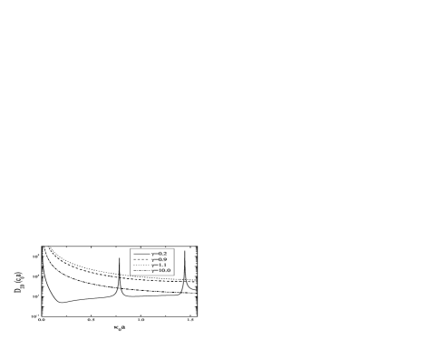
Figure 2: Diffusion constant of the 2D disordered medium in units of $c_{0}a$, as a function of the dimensionless frequency $\kappa_{0}a$ for four different scatterer-medium velocity ratios ($\gamma$). The scatterer density is determined by setting $\left\langle d_{s}\right\rangle/a=10$.

The diffusion constants in 1D and 3D media show the same behavior. Of course, the resonances at low velocity, are caused by the fact that all scatterers are assumed to have equal size. When scatterer sizes (or velocities) are allowed to vary, the resonances will be averaged out.

When the scatterer velocity is zero we obtain an impenetrable model scatterer. This is not a useful model scatterer, as in the low frequency range the mean free path (and thus the diffusion constant) differ considerably from the penetrable scatterer case. The reason for this is that the limits for $\omega\rightarrow 0$ and $\gamma\rightarrow 0$ do not commute, as

$$\lim_{\omega\rightarrow 0}\lim_{\gamma\rightarrow 0}\ell_{f}=\text{constant,}$$ (74)

while

$$\lim_{\gamma\rightarrow 0}\lim_{\omega\rightarrow 0}\ell_{f}=\infty\text{.}$$ (75)

The effect of this is that at the longer wavelengths, $\ell_{f}$ for the impenetrable scatterer is orders of magnitude smaller than $\ell_{f}$ for non-zero values of $\gamma$.

VII Conclusions

We have calculated the transport of energy and intensity in disordered 1D, 2D and 3D (infinite) media emitted by a monochromatic source. Using the ladder approximation to the Bethe-Salpeter equation we explicitly show that the total intensity is well approximated by the sum of the coherent and the fully developed diffuse wave field, for all source-receiver distances. Energy transport and intensity propagation in 2D disordered systems shows interestingly different behavior compared to the 3D case: In 2D, the average energy flux depends on the mean free path and the effective transport velocity depends differently in terms of the scattering parameters. The (gradient of the) intensity as a function of the source-receiver distance, on the other hand, behaves similarly in the 2D and the 3D case. The monochromatic source enables us to investigate the frequency dependence due to finite size scatterers on the macroscopic diffusion constant. For a monodisperse distribution of scatterers shape resonances show up in the relevant frequency range for low internal scatterer velocities ($\gamma$ small). In this frequency range (where scattering is expected to be isotropic) the dependence of the scattering properties on frequency can not be neglected. This means that descriptions of broadband pulse propagation through these media should in principle incorporate both frequency dependent and multiple scattering effects. The development of a workable Ward identity in this case remains a challenge, however. Finally, we want point out that our model describes transport of scalar acoustic waves but results can be extended and many conclusions should also apply to vector wave fields random media.

Appendix A Energy and intensity in 2D

In this appendix we derive the configuration-averaged intensity and energy flux in a disordered 2D medium. Starting point is the 2D Green function propagator

$$G\left(r;\omega\right)=\left\{\begin{array}[c]{c}-\frac{i}{4}H_{0}^{(1)}\left(\left(\kappa_{r}+i/\left(2\ell_{f}\right)\right)r\right)\text{ \ \ if \ }\omega>0\\ \frac{i}{4}H_{0}^{(2)}\left(\left(\kappa_{r}-i/\left(2\ell_{f}\right)\right)r\right)\text{ \ \ \ \ if \ }\omega<0\end{array}\right.\text{.}$$ (76)

We use the properties

$$H_{0}^{(2)}\left(\left(\kappa_{r}-i/\left(2\ell_{f}\right)\right)r\right)$$

$$=H_{0}^{(1)}\left(\left(-\kappa_{r}+i/\left(2\ell_{f}\right)\right)r\right)\text{,}$$ (77)

and

$$H_{0}^{(1)}\left(\left(\pm\kappa_{r}+i/\left(2\ell_{f}\right)\right)r\right)$$

$$=-i\frac{2}{\pi}K_{0}\left(\left(\mp i\kappa_{r}+1/\left(2\ell_{f}\right)\right)r\right)\text{,}$$ (78)

to express the Hankel functions ($H_{0}^{(j)}$) in terms of modified Bessel function of the second kind ($K_{0}$). The Fourier transform of the coherent intensity

$$\Pi_{0}\left(k;\omega\right)=2\pi{\displaystyle\int\limits_{0}^{\infty}}\left|G\left(r;\omega\right)\right|^{2}J_{0}\left(kr\right)\text{,}$$ (79)

is then obtained from Ref. gr1  and using properties of the associated Legendre polynomials as1  as

$$\Pi_{0}\left(k;\omega\right)=\frac{\ell_{f}^{2}}{\pi}\frac{1}{1+\left(2\kappa_{r}\ell_{f}\right)^{2}}\frac{P_{-1/2}^{-1/2}\left(u\right)}{P_{1/2}^{-1/2}\left(u\right)}\text{,}$$ (80)

with

$$u=\frac{1-\left(2\kappa_{r}\ell_{f}\right)^{2}}{1+\left(2\kappa_{r}\ell_{f}\right)^{2}}+\frac{2k\ell_{f}}{1+\left(2\kappa_{r}\ell_{f}\right)^{2}}\text{.}$$ (81)

This is can be rewritten as

$$\Pi_{0}\left(k;\omega\right)=\frac{\ell_{f}^{2}}{\pi}\frac{\arcsin\left(\frac{\sqrt{\left(2\kappa_{r}\ell_{f}\right)^{2}-\left(k\ell_{f}\right)^{2}}}{\sqrt{1+\left(2\kappa_{r}\ell_{f}\right)^{2}}}\right)}{\sqrt{1+\left(k\ell_{f}\right)^{2}}\sqrt{\left(2\kappa_{r}\ell_{f}\right)^{2}-\left(k\ell_{f}\right)^{2}}}\text{.}$$ (82)

$\Pi_{0}\left(k;\omega\right)$ is real, continuous and differentiable for all (real) $k\geq 0$.

The flux in the 2D system is given by

$$\left\langle\mathbf{n\cdot F}_{\omega}\left(\mathbf{r}\right)\right\rangle=\frac{Q^{2}\rho_{0}\omega}{2}\frac{C}{r}\mathbf{n}\cdot\widehat{\mathbf{r}}\text{,}$$ (83)

where $C$ is the constant to be calculated:

$$C=\frac{{\displaystyle\int\limits_{0}^{\infty}}dr\operatorname{Im}\left\{G\left(r;\omega\right)\partial_{r}G^{\ast}\left(r;\omega\right)\right\}r^{2}}{\Pi_{0}^{-1}\left(k=0;\omega\right)\left.\partial_{k}^{2}\Pi_{0}\left(k;\omega\right)\right|_{k=0}}\text{.}$$ (84)

The term in the denominator is easily obtained

$$\Pi_{0}^{-1}\left(k=0;\omega\right)\left.\partial_{k}^{2}\Pi_{0}\left(k;\omega\right)\right|_{k=0}$$

$$=-\ell_{f}^{2}\left(1-\frac{1}{\left(2\kappa_{r}\ell_{f}\right)^{2}}+\frac{1}{2\kappa_{r}\ell_{f}\arctan\left(2\kappa_{r}\ell_{f}\right)}\right)\text{.}$$ (85)

The solution to the integral

$${\displaystyle\int\limits_{0}^{\infty}}dr\operatorname{Im}\left\{G\left(r;\omega\right)\partial_{r}G^{\ast}\left(r;\omega\right)\right\}r^{2}$$

$$=-\frac{sgn\left(\omega\right)}{4\pi^{2}\ell_{f}}{\displaystyle\int\limits_{0}^{\infty}}drr^{2}\operatorname{Im}\left\{\left(i\kappa_{r}+1/\left(2\ell_{f}\right)\right)\right.$$

$$\left.\times K_{0}\left(\left(-i\kappa_{r}+1/\left(2\ell_{f}\right)\right)r\right)K_{1}\left(\left(i\kappa_{r}+1/\left(2\ell_{f}\right)\right)r\right)\right\}$$

$$=-\frac{sgn\left(\omega\right)}{4\pi^{2}\ell_{f}^{2}}\operatorname{Im}\left\{2\frac{\left(1+i2\kappa_{r}\ell_{f}\right)^{2}}{\left(1-i2\kappa_{r}\ell_{f}\right)^{4}}\right.$$

$$\left.\times F\left(2,2;3;1-\frac{\left(1+i2\kappa_{r}\ell_{f}\right)^{2}}{\left(1-i2\kappa_{r}\ell_{f}\right)^{2}}\right)\right\}\text{,}$$ (86)

can be found from Ref. gr1 . However, the proper solution (on the right Riemann sheet) needs to be chosen in order to simplify the hypergeometric series $F$. One can check numerically that

$${\displaystyle\int\limits_{0}^{\infty}}dr\operatorname{Im}\left\{G\left(r;\omega\right)\partial_{r}G^{\ast}\left(r;\omega\right)\right\}r^{2}$$

$$=-\frac{sgn\left(\omega\right)}{4\pi^{2}\ell_{f}^{2}}\arctan\left(2\kappa_{r}\ell_{f}\right)$$

$$\times\left(1-\frac{1}{\left(2\kappa_{r}\ell_{f}\right)^{2}}+\frac{1}{2\kappa_{r}\ell_{f}\arctan\left(2\kappa_{r}\ell_{f}\right)}\right)\text{.}$$ (87)

Hence, $C$ is given by

$$C=\frac{sgn\left(\omega\right)}{4\pi^{2}}\arctan\left(2\kappa_{r}\ell_{f}\right)\text{.}$$ (88)

The intensity is proportional to the propagator $\Pi\left(r;\omega\right)$, expressed in terms of $\Pi_{0}\left(k;\omega\right)$ by the Fourier transform (46). Only the gradient of the intensity is a well-defined property, so we calculate

$$\nabla\Pi\left(r;\omega\right)=-\widehat{\mathbf{r}}{\displaystyle\int\limits_{0}^{\infty}}\frac{dk}{2\pi}\frac{k^{2}J_{1}\left(kr\right)}{\Pi_{0}^{-1}\left(k;\omega\right)-\Pi_{0}^{-1}\left(k=0;\omega\right)}\text{.}$$ (89)

This part contains both the coherent and the scattered intensity. As the coherent intensity is known, we focus on the scattered intensity by calculating

$$\nabla\Pi_{sc}\left(r;\omega\right)=-\widehat{\mathbf{r}}{\displaystyle\int\limits_{0}^{\infty}}\frac{dk}{2\pi}J_{1}\left(kr\right)k^{2}\Pi_{sc}\left(k;\omega\right)\text{,}$$ (90)

with

$$\Pi_{sc}\left(k;\omega\right)=\frac{\Pi_{0}^{-1}\left(k=0;\omega\right)\Pi_{0}\left(k;\omega\right)}{\Pi_{0}^{-1}\left(k;\omega\right)-\Pi_{0}^{-1}\left(k=0;\omega\right)}\text{.}$$ (91)

(90) is the integral to calculate numerically when we want to calculate the gradient of the multiply scattered intensity. $\Pi_{sc}\left(k;\omega\right)$ is a monotonically decaying function with a maximum at $k=0$, that vanishes as $k\rightarrow\infty$. As the Bessel function is also decaying with $r$, we know that for $r/\ell_{f}\gg 1$

$$\nabla\Pi_{td}\left(r;\omega\right)=-\widehat{\mathbf{r}}\frac{\Pi_{sc}\left(k=0;\omega\right)}{2\pi r}\text{.}$$ (92)

and

$$\nabla\Pi_{td}\left(r\right)=-\widehat{\mathbf{r}}\frac{\arctan\left(2\kappa_{r}\ell_{f}\right)}{\pi^{2}2\kappa_{r}\ell_{f}}\frac{1}{r}g^{-1}\left(2\kappa_{r}\ell_{f}\right)\text{,}$$ (93)

where

$$g\left(2\kappa_{r}\ell_{f}\right)=1-\frac{1}{\left(2\kappa_{r}\ell_{f}\right)^{2}}+\frac{1}{2\kappa_{r}\ell_{f}\arctan\left(2\kappa_{r}\ell_{f}\right)}\text{.}$$ (94)

$td$ stands for “totally diffusive”.

References

• (1) Photon Migration and Imaging in Random Media and Tissues, edited by B. Chance and R.R. Alfano (Proc. SPIE, Vol. 1888, 1993); S.R. Arridge, Inverse Problems 15, R41, (1999)
• (2) A.K. Fung, Microwave Scattering and Emission Models and Their Applications (Artech House, Boston, 1994)
• (3) F.J. Fry, Ultrasound: Its Applications in Medicine and Biology (Elsevier, Amsterdam, 1978); A. Migliori and J.L. Sarrao, Resonant Ultrasound Spectroscopy, Applications to Physics, Materials Measurement and Nondestructive Evaluation (Wiley, New York, 1997)
• (4) R. Snieder, in Diffuse Waves in Complex Media, edited by J.P. Fouque (Kluwer, Dordrecht, 1999)
• (5) E. Larose, A. Derode, M. Campillo and M. Fink, J. Appl. Phys. 95, 8393 (2004)
• (6) P. Sheng, Introduction to Wave Scattering, Localization and Mesoscopic Phenomena (Academic Press, New York, 1995)
• (7) D.S. Wiersma, P. Bartolini, A. Lagendijk and R. Righini, Nature 390, 671 (1997)
• (8) M. Haney and R. Snieder, Phys. Rev. Lett. 91, 093902 (2003); S.E. Skipetrov and B.A. van Tiggelen, ibid. 92, 113901 (2004); S.K. Cheung, X. Zhang, Z.Q. Zhang, A.A. Chabanov and A.Z. Genack, ibid. 92, 173902 (2004); E. Larose, L.Β Margerin, B.A. van Tiggelen and M. Campillo, ibid. 93, 048501 (2004)
• (9) K.M. Yoo, F.Liu and R.R. Alfano, Phys. Rev. Lett. 64, 2647 (1990); R.H.J. Kop, P. de Vries, R. Sprik, A. Lagendijk, ibid. 79, 4369 (1997); P.-A. Lemieux, M.U. Vera and D.J. Durian, Phys. Rev. E 57, 4498 (1998); Z.Q. Zhang, I.P. Jones, H.P. Schriemer, J.H. Page, D.A. Weitz, and P. Sheng, ibid. 60, 4843 (1999); X. Zhang and Z.Q. Zhang, ibid. 66, 016612 (2002)
• (10) M. Fink, Phys. Today 50, 34 (1997)
• (11) P. de Vries, D.V. van Coevorden and A. Lagendijk, Rev. Mod. Phys. 70, 447 (1998)
• (12) M.C.W. van Rossum and Th.M. Nieuwenhuizen, Rev. Mod. Phys. 71, 313 (1999)
• (13) G.E.W. Bauer, M.S. Ferreira, and C.P.A. Wapenaar, Phys. Rev. Lett. 87, 113902 (2001)
• (14) H. Sato and M.C. Fehler, Seismic Wave Propagation and Scattering in the Heterogeneous Earth (Springer, New York, 1998)
• (15) A. Tourin, M. Fink, and A. Derode, Waves in Random Media 10, R31 (2000)
• (16) A. Lagendijk and B.A. van Tiggelen, Physics Reports 270, 143 (1996)
• (17) R. Hennino, N. TrΓ©gourΓ¨s, N.M. Shapiro, L. Margerin, M.Campillo, B.A. van Tiggelen and R.L.Β Weaver, Phys. Rev. Lett. 86, 3447 (2001); U. Wegler and B.-G. LΓΌhr, Geophys. J. Int. 145, 579 (2001)
• (18) A. Tourin, A. Derode, P. Roux, B.A. van Tiggelen and M. Fink, Phys. Rev. Lett. 79, 3637 (1997); N.P. TrΓ©gourΓ¨s and B.A. van Tiggelen, Phys. Rev. E 66, 036601 (2002); G. Samelsohn and V. Freilikher, ibid. 70, 046612 (2004)
• (19) R. Sprik and A. Tourin, Ultrasonics 42, 775 (2004)
• (20) A. Messiah, Quantum Mechanics, Volume II (North-Holland, Amsterdam, 1962)
• (21) E. Merzbacher, Quantum Mechanics (Wiley, New York, 1961)
• (22) P.Β Exner and P. Ε eba, Phys. Lett. A 222, 1 (1996)
• (23) M.S. Ferreira and G.E.W. Bauer, Phys. Rev. E 65, 045604(R) (2002)
• (24) I.S. Gradshteyn and I.M. Ryzhik, Table of Integrals, Series and Products (Academic Press, London, 1965)
• (25) M. Abramowitz and I.A. Stegun, Handbook of Mathematical Functions (Dover Publications, New York, 1964)