Magnetic resonance study of the spin-reorientation transitions in the quasi-one-dimensional antiferromagnet BaCu₂Si₂O₇.

Abstract

A quasi-one dimensional antiferromagnet with a strong reduction of the ordered spin component, BaCu₂Si₂O₇, is studied by the magnetic resonance technique in a wide field and frequency range. Besides of conventional spin-flop transition at the magnetic field parallel to the easy axis of spin ordering, magnetic resonance spectra indicate additional spin-reorientation transitions in all three principal orientations of magnetic field. At these additional transitions the spins rotate in the plane perpendicular to the magnetic field keeping the mutual arrangement of ordered spin components. The observed magnetic resonance spectra and spin-reorientation phase transitions are quantitatively described by a model including the anisotropy of transverse susceptibility with respect to the order parameter orientation. The anisotropy of the transverse susceptibility and the strong reduction of the anisotropy energy due to the quantum spin fluctuations are proposed to be the reason of the spin reorientations which are observed.

I Introduction

Low dimensional spin systems have been actively studied during the last few decades. This non-vanishing interest is due to the increasing role of quantum fluctuations in these magnets, which can lead to the formation of non-trivial ground sates. One-dimensional antiferromagnetic spin chains are known to remain in a quantum-disordered state down to zero temperature. However, a weak inter-chain interaction makes the formation of Neel order again possible.

The formation of Neel order in these quasi-one-dimensional magnets is characterized by two features: Firstly, the transition temperature $T_{N}$ is much smaller than the temperature corresponding to the in-chain exchange integral. Secondly, the sublattice magnetization (average spin value per site) is strongly reduced with respect to the nominal value.

The recently studied oxide BaCu₂Si₂O₇ is a good example of a spin S=1/2 quasi-one-dimensional antiferromagnet. The exchange integral values determined by inelastic neutron scattering Kenzelmann are $J$=24.1meV for the in-chain interaction and $J_{a}$=-0.46meV, $J_{b}$=0.20meV, $J_{[110]}$=0.076meV for different inter-chain interactions. The ordering temperature is $T_{N}$=9.2K. Susceptibility data tsukada:2sf reveal that the $c$ axis is the easy axis of the spin ordering. The ordered magnetic moments at lattice sites were found to be equal to 0.15$\mu_{B}$ at zero magnetic field.Kenzelmann ; zheludev:struct Thus a strong spin reduction by zero point fluctuations is present in this material.

The interest for the magnetic order observed in BaCu₂Si₂O₇ was enhanced by the observation of unusual spin-reorientation transitions: when the magnetic field is applied along the easy anisotropy axis two spin-reorientation transitions were observed tsukada:2sf at the fields $H_{c1}$=20 kOe and $H_{c2}$=49 kOe. Later, another phase transition at $H_{c3}$=78 kOe was reported for $\mathbf{H}||b$,poirier:sf3 i.e. when the field is perpendicular to the easy axis. The magnetic structure at $\mathbf{H}||c$ was identified with the help of elastic neutron scattering experiments:zheludev:struct at low fields, $H<H_{c1}$, the local magnetic moments are aligned antiferromagnetically along the $c$-axis. At the first transition (at $H_{c1}$) they rotate to the $(ab)$ plane and align along the $b$ axis. Finally, at the second transition field, $H_{c2}$, the antiferromagnetic vector is rotated within the $(ab)$ plane towards the $a$ axis. Neglecting a small spin canting in the high-field phases, the exchange spin structure (mutually parallel or antiparallel orientation of the local magnetic moments) remains the same in all three phases.

The observation of the spin-reorientation transitions at $H_{c2}$ and $H_{c3}$ is surprising for a supposedly collinear antiferromagnet. Usually a collinear easy-axis antiferromagnet exhibits only a spin-reorientation known as a spin-flop when the magnetic field is applied parallel to the easy axis. At the spin-flop point, the antiferromagnetic order parameter rotates from the easy axis to a perpendicular direction, and the loss in anisotropy energy is compensated by the gain in magnetization energy due to the large transverse susceptibility.

A unique spin-reorientation transition when the field is applied perpendicular to the easy axis of a collinear antiferromagnet, was reported earlier for K₂V₃O₈.kvo Here, a weak ferromagnetic moment arises if the antiferromagnetic order parameter is tilted apart from the easy axis aligned along the high order symmetry axis. In this case the gain in Zeeman energy is due to the appearance of a weak ferromagnetic moment. This is not the case of BaCu₂Si₂O₇: no signs of a ferromagnetic magnetization in high-field phases were present, and, moreover, the identified antiferromagnetic structure is not compatible with weak ferromagnetism. glazkov

In the theoretical model of Ref.glazkov, two additional phase transitions observed in BaCu₂Si₂O₇ were explained by a relatively strong dependence of the transverse susceptibility on the direction of the order parameter. The resulting anisotropic part of the Zeeman energy exceeds the change in energy of magnetic anisotropy above the corresponding critical fields. However, the origin of this anisotropy, as well as the reasons for the increase of its influence, are still not understood.

The magnetic resonance technique enables one to explore low-energy dynamics of magnetic crystals by sensitive and precise measurement of the resonance frequency and polarization of $\mathbf{q}=0$ excitations. At spin-reorientation transitions the local ordered moments rotate by a noticeable angle, and, at the exact field value, this rotation costs no energy. Thus, the corresponding mode of the spin resonance is softening at the transition field and its frequency turns to zero. Therefore the observation of the magnetic resonance soft modes appears to be a powerful tool to study spin-reorientation transitions.

We present here a detailed magnetic resonance study of BaCu₂Si₂O₇, which is essentially complementary to earlier data of Refs. jpsj-afmr, ; hayn-afmr, . We have observed the soft modes of the antiferromagnetic resonance (AFMR), marking the mentioned spin-reorientation transitions for $\mathbf{H}||c$ and $\mathbf{H}||b$. Besides, we report on the spin-reorientation transition for $\mathbf{H}||a$, at a magnetic field of 110 kOe, which has not been observed before. We present a model based on the macroscopic approach to the spin dynamics of an antiferromagnet which describes quantitatively the observed AFMR spectra and the field-induced phase transitions. The model includes the anisotropy of the transverse susceptibility with respect to the order parameter orientation. We discuss the possible origin of this anisotropy and the possible increase of its influence because of the strong reduction of the ordered moments by quantum fluctuations.

II Experimental technique and samples preparation.

Magnetic resonance was studied using a set of home-made ESR spectrometers with transmission type resonators covering the frequency range 9–110 GHz, equipped with He-cooled cryomagnets for 8 and 14T. Magnetic resonance lines were recorded by measurements of the field-dependences of the microwave power transmitted through the resonator with the sample.

Single crystalline samples of BaCu₂Si₂O₇, several centimeters long, were grown by the floating zone technique poirier:sf3 , from which samples of about 2x2x3 mm³ were cut and used for our microwave experiments. Crystals were oriented by a conventional x-ray diffraction method. Because the lattice parameters for $a$ and $c$ directions are very close ($a$=6.862Å $b$=13.178Å, $c$=6.891Å cryst-struct ), only $b$ axis can be easily unambiguously identified. The axis $a$ and $c$ were distinguished by the behaviour in the magnetic field using the data of Ref.tsukada:2sf, , where $c$ axis was identified as an easy axis of magnetic ordering.

III Experimental results

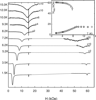
Figure 1: Temperature dependence of the ESR absorption spectrum at $f=44.04$GHz and $\mathbf{H}||b$. Dashed lines are guides to the eye connecting separately measured low-field and high-field parts of the ESR absorption spectrum. High-field parts of the T=5.2 K, 6.2 K and 7.2 K curves are Y-stretched with the corresponding coefficient. The narrow absorption line at $H=$15.7 kOe is a DPPH mark ($g=2.0$). Insert: temperature dependence of the two resonance fields.

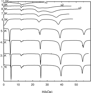
Figure 2: Temperature dependence of the ESR absorption spectrum at $f=38.25$GHz and with $\mathbf{H}||c$.

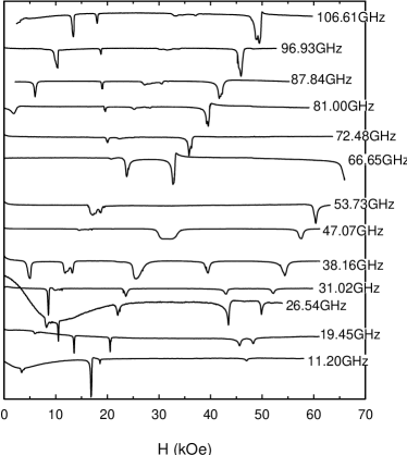
Figure 3: ESR absorption spectrum at different microwave frequencies. $\mathbf{H}||c$, T=1.5K.

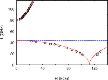
Figure 4: (color online) Field dependence of the antiferromagnetic resonance frequency at $\mathbf{H}||a$ and $T=$1.5 K. Circles represent experimental points of resonance absorption and solid lines — theory (see text). Dashed line is the $f(H)$ dependence calculated for a two sublattices antiferromagnet with the same zero-field gaps.

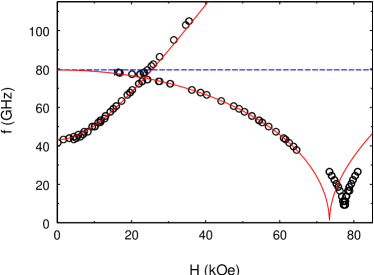
Figure 5: (color online) Field dependence of the antiferromagnetic resonance frequency at $\mathbf{H}||b$, and $T=$1.5K. Circles are experimental points and solid line is theoretical calculation (see text). Dashed lines is the $f(H)$ dependence of a two sublattices antiferromagnet with the same zero-field gaps.

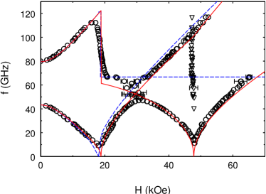
Figure 6: (color online) Field dependence of the antiferromagnetic resonance frequency at $\mathbf{H}||c$, $T=$1.5 K. Circles represent experimental points of resonance absorption, triangles — non-resonance response at the spin-reorientation transition, solid line — theory (see text). Dashed lines is the $f(H)$ dependence calculated for a two sublattices antiferromagnet with the same zero-field gaps.

The temperature evolution of the resonance absorption spectrum at $\mathbf{H}||b$ is shown at Figure 1. At $T\geq 9.3K$, a broad resonance line with a g-factor slightly above 2.0 is observed. The absorption spectrum changes when crossing the transition temperature $T_{N}=9.2K$. The maximum of absorption shifts to lower fields and another absorption line appears at a higher field. The temperature dependence of the resonance field for both resonance lines is shown in the insert of the Fig. 1. The temperature at which the low-field absorption line begins to shift corresponds well to $T_{N}$. When the field is applied along the easy axis (see Fig. 2) a multi-component absorption spectrum develops below $T_{N}$.

An additional absorption signal of irregular shape is clearly visible on Fig. 2 at a field close to 13 kOe. Its intensity increases with decreasing temperature and its position is temperature independent. Probably it is due to a paramagnetic impurity or to a small amount of another phase.

Magnetic resonance absorption curves, taken at different frequencies, are illustrated in Fig. 3. The frequency-field dependences $f(H)$ are shown at Figures 4—6. Two modes of resonance absorption with zero-field gaps of approximately 42 and 80 GHz are observed for all three orientations of the magnetic field. The low-field spectra are in good agreement with the $f(H)$ dependences of a conventional two-sublattice antiferromagnet, Kubo-afmr which are represented by dashed lines in Figs. 4—6: when the magnetic field is applied parallel to the easy axis a characteristic spin-flop transformation of the spectrum, with a vertical frequency drop, occurs at $H_{c1}=(18.8\pm 0.8)$kOe. For the other directions, in the low-field range $H\leq$20 kOe there is one mode with a strong field dependence of the resonance frequency and one mode with an approximately constant frequency. At $\mathbf{H}||a$ the resonance mode with a strong field dependence starts from the larger zero-field gap, while at $\mathbf{H}||b$ the larger gap corresponds to a mode with a weak field dependence of the resonance frequency. This low-field behavior allows to identify the $a$ axis as a hard axis of antiferromagnetic ordering and $b$ axis — as a middle axis of spin ordering according to Ref. Kubo-afmr, .

However, upon increasing the magnetic field, an additional softening of one of the two modes occurs. An additional softening occurs for the easy-axis orientation of the applied field ($\mathbf{H}||c$) at the field $H_{c2}=(47.8\pm 1.0)$kOe, for the $\mathbf{H}||b$ at the field $H_{c3}=(77.4\pm 0.8)$kOe, and for the $\mathbf{H}||a$ orientation at the field $H_{c4}=(110\pm 5)$kOe.

The values of the spin-reorientation fields $H_{c2}$ and $H_{c3}$ are in good agreement with that reported in Refs. tsukada:2sf, ; poirier:sf3, . Softening of the AFMR modes at these fields was reported also in Refs. hayn-afmr, ; jpsj-afmr, (note that the orientations $\mathbf{H}||a$ and $\mathbf{H}||b$ are mixed in Fig.12 of Ref.jpsj-afmr, ). The last spin-reorientation transition, observed at $\mathbf{H}||a$ ($H_{c4}$), was not reported before.

IV Discussion.

IV.1 Rotations of the order parameter.

The softening of spin-resonance modes indicates spin-reorientation transitions, since at the transition field the rotation of the spins costs no energy. Comparison of the observed antiferromagnetic resonance frequency-field dependences with the results of the conventional two-sublattice model Kubo-afmr is shown in Figs. 4—6. This matching allows one to draw simple conclusions on the directions of the order parameter rotation at the observed spin-reorientation transitions.

The standard model of the two-sublattices antiferromagnet includes the anisotropy energy $a_{1}l_{x}^{2}+a_{2}l_{y}^{2}$ ($l_{\alpha}$ are order parameter components) and the Zeeman energy resulting from the transverse susceptibility. This model yields only the spin-flop transition at the magnetic field applied parallel to the easy axis of spin ordering. At the spin-flop point the spins rotate from the easy axis to the perpendicular direction. There are 8 magnetic ions in the unit cell of BaCu₂Si₂O₇, therefore this compound should be a multi-sublattice antiferromagnet. Nevertheless, the low-frequency dynamics of the collinear antiferromagnet in a weak magnetic field is described by a universal equation which does not depend on the number of sublattices.Andreev-Marchenko Therefore, at low fields, i.e. reasonably below $H_{c2,c3,c4}$, one can use the classification of the AFMR modes in terms of the order parameter oscillations in a two-sublattice antiferromagnetKubo-afmr .

At the field $H_{c1}$ the magnetic resonance mode starting from the lower gap is softening. In the two-sublattice model this mode corresponds to the oscillations of the order parameter in the direction from the easy axis towards the second-easy axis. Softening of this mode means the free rotation of the order parameter from easy axis to the second-easy axis, as at the conventional spin-flop transition. Further, the data presented on Figs.4-6 indicate that the AFMR softening observed at the fields $H_{c2,c3,c4}$ corresponds to the field-independent resonance modes of the two-sublattice antiferromagnet. These field-independent modes are oscillations of the order parameter in the plane which is perpendicular to the magnetic field. Thus, the softening of the AFMR modes at the fields $H_{c2,c3,c4}$ reveal the spin rotation around the the field direction. These conclusion is in agreement with the change of the magnetic structure at the transition field $H_{c2}$, derived from elastic neutron scattering.zheludev:struct The above identification of resonance modes indicates that when $\mathbf{H}||a$ and $\mathbf{H}||b$ the spin reorientations correspond to the rotation of the order parameter from the easy axis $c$ to the direction of $b$ and $a$ axes, correspondingly.

IV.2 Antiferromagnetic resonance theory.

The comparison of our results with the simple two-sublattice model allows to draw the above qualitative conclusions about the spin rotations at the observed phase transitions. Below we give a quantitative description of the observed antiferromagnetic resonance frequencies. While obeying the two sublattice model in low fields, the multisublattice antiferromagnet like BaCu₂Si₂O₇ may, in principle, change the exchange spin structure in high fields of about the exchange field value. Therefore we should check at first, whether the observed spin-reorientation transitions conserve the exchange spin structure (i.e. the mutual alignment of the ordered spin components).

The field range of the present experiment is well below the value of the main exchange field $H_{E}\sim J/\mu_{B}\sim 4\cdot 10^{3}$kOe derived from the in-chain exchange integral $J=$24.1meV. In the same time, the interchain exchange integrals may be of the order of the applied fields. However, the change of the low-field exchange structure at the fields $H_{c1,c2,c3,c4}$ may be excluded by the following experimental observations. At first, the elastic neutron scattering experiment zheludev:struct performed at the easy-axis orientation of the applied field has revealed that the main component of the antiferromagnetic order parameter corresponds to the same mutual alignment of spins in all three phases. Second, as described above, we observe at the fields $H_{c1,c2,c3,c4}$ the softening of the lowest resonance modes with the gaps of the anisotropic nature, analogous to the modes of a two sublattice antiferromagnet, while at the change of the exchange structure the modes of the exchange origin should be softened. The exchange modes of multisublattice antiferromagnets ExchangeModes , corresponding to the oscillations of the mutual orientations of the ordered moments have usually much higher frequencies, of the order of $J/h$, while the frequencies of lowest $q=0$ spin waves are zero in the absence of anisotropy. The high-frequency ESR measurements jpsj-afmr have found resonance mode at a frequency of about 400 GHz in the field range below 150 kOe which probably softens in a field near 250 kOe. This is clearly one of the exchange modes. We consider it as the lowest exchange mode. The magnetic field value $H^{*}=$250kOe can be taken as a measure of the exchange field corrected for the low-dimensionality. The field range of the present experiment is at least two times smaller than $H^{*}$.

Thus, we suppose in the further analysis, that the zero-field exchange structure remains the same in the whole field range of the described experiment. Under this condition, a macroscopic (hydrodynamic) approach to the spin dynamics Andreev-Marchenko is valid. As a first step of this approach we write down the potential energy of the antiferromagnet as a function of the orientation of the order parameter and magnetic field. The potential energy expansion includes usually the anisotropy energy and Zeeman energy. These terms are responsible for the conventional spin-flop transition in the easy-axis orientation of the magnetic field. To include additional spin-reorientation transitions we phenomenologically add the higher order invariants allowed by the crystal symmetry ($D_{2h}^{16}$) and by the spin-order parameter. The eight-sublattice order parameter was found in the experimentzheludev:struct and has the form of ${\bf l}_{6}$ in terms of Ref. glazkov, . This structure is not compatible with weak ferromagnetism.glazkov Thus, the potential energy contains only terms of even power of $l_{\alpha}$ and $H_{\alpha}$. As shown in Ref. glazkov, , terms quadratic on both $l_{\alpha}$ and $H_{\alpha}$ should be added to explain additional transitions.

We consider in zero-temperature limit the following form of the potential energy (here the exchange part of the transverse magnetic susceptibility is set to unity, ${\bf l}$ is the unit vector in the direction of the order parameter):

$$U = -\frac{1}{2}\bigl{[}\mathbf{l}\times\mathbf{H}\bigr{]}^{2}+a_{1}l_{x}^{2}+a_{2}l_{y}^{2}+\xi_{1}\bigl{(}\mathbf{H}\cdot\mathbf{l}\bigr{)}H_{x}l_{x}+$$ (1)

$$+\xi_{2}\bigl{(}\mathbf{H}\cdot\mathbf{l}\bigr{)}H_{y}l_{y}-(\xi_{1}+\xi_{2})\bigl{(}\mathbf{H}\cdot\mathbf{l}\bigr{)}H_{z}l_{z}-$$

$$-B_{1}H_{x}^{2}(l_{y}^{2}-l_{z}^{2})-B_{2}H_{y}^{2}(l_{x}^{2}-l_{z}^{2})-B_{3}H_{z}^{2}(l_{x}^{2}-l_{y}^{2})+$$

$$+C_{1}H_{y}H_{z}l_{y}l_{z}+C_{2}H_{x}H_{z}l_{x}l_{z}+C_{3}H_{x}H_{y}l_{x}l_{y}$$

the Cartesian coordinates are chosen as $x||a$, $y||b$, $z||c$. The first three terms are Zeeman energy and magnetic anisotropy energy, $a_{1}>a_{2}>0$ are anisotropy constants corresponding to the observed hierarchy of the anisotropy axes in weak fields. These terms describe adequately the observed low-field behaviour with the characteristic features of a collinear antiferromagnet. Other terms represent all symmetry-allowed invariants quadratic in components of $\mathbf{H}$ and $\mathbf{l}$. The three invariants with $\xi_{i}$ coefficients are of exchange-relativistic origin: they contain the scalar product $\bigl{(}\mathbf{l}\cdot\mathbf{H}\bigr{)}$, which is invariant under simultaneous rotation of the order parameter and the magnetic field. Other terms are of relativistic (spin-orbital) nature, they are not invariant under simultaneous rotations of magnetic vectors.

Equation (1) is written just phenomenologically, we do not consider the hierarchy of the relativistic terms. Potential energy (1) differs from that of Ref. glazkov, , where only two exchange-relativistic terms $\mathbf{H}^{2}l_{x}^{2}$ and $\mathbf{H}^{2}l_{y}^{2}$ were taken into account instead of the six terms with the $B_{i}$ and $C_{i}$ coefficients in Eqn. (1). Other terms were neglected because they should be smaller than exchange-relativistic terms. However, the model of Ref. glazkov, does not describe the spin-reorientation transition at $\mathbf{H}||a$ ($H_{c4}$). We show below in sec. C, that the coefficients $B_{i}$, $C_{i}$ are of the same order in spin-orbital coupling.

Minimization of the energy (1) in the exact orientations of the magnetic field yields for the fields of spin-reorientation transitions:

$$\mathbf{H}||z,~{}\mathbf{l}||z\leftrightarrow\mathbf{l}||y : H_{c1}^{2}=\frac{2a_{2}}{1-2(\xi_{1}+\xi_{2})-2B_{3}}$$ (2)

$$\mathbf{H}||z,~{}\mathbf{l}||y\leftrightarrow\mathbf{l}||x : H_{c2}^{2}=\frac{a_{1}-a_{2}}{2B_{3}}$$ (3)

$$\mathbf{H}||y,~{}\mathbf{l}||z\leftrightarrow\mathbf{l}||x : H_{c3}^{2}=\frac{a_{1}}{2B_{2}}$$ (4)

$$\mathbf{H}||x,~{}\mathbf{l}||z\leftrightarrow\mathbf{l}||y : H_{c4}^{2}=\frac{a_{2}}{2B_{1}}$$ (5)

The transition at $H_{c1}$ is the normal spin-flop transition, it occurs when the gain in magnetization energy due to the large transverse susceptibility exceeds the loss in anisotropy energy. Other transitions result from the gain in the magnetization energy due to the small difference of the transverse susceptibility in the phases with different orientations of the antiferromagnetic vector. Directions of the order parameter rotation at these transitions are in agreement with the results of previous subsection.

The dynamics of the collinear antiferromagnet in zero temperature limit is described Andreev-Marchenko by the equation:

$$\frac{\partial}{\partial t}\bigl{[}\mathbf{l}\times\mathbf{\dot{l}}\bigr{]}=\gamma^{2}\bigl{[}\mathbf{l}\times\mathbf{H_{l}}\bigr{]}+2\gamma\bigl{(}\mathbf{l}\cdot\mathbf{H}\bigr{)}\mathbf{\dot{l}}$$ (6)

here $\mathbf{H_{l}}=-\partial U/\partial\mathbf{l}$, exchange part of the transverse susceptibility is set to unity as before. Linearizing equation (6) near the equilibrium spin configuration and solving for eigenfrequencies, we obtain the following expressions for the AFMR frequency-field dependences at the exact orientations of the magnetic field:
for $\mathbf{H}||x$ (hard axis of magnetization):
$H<H_{c4}$:

$$\frac{\nu_{1}^{2}}{\gamma^{2}} = \bigl{(}1+2\xi_{1}\bigr{)}H^{2}+2a_{1}-a_{2}\left(\frac{H}{H_{c4}}\right)^{2}$$ (7)

$$\frac{\nu_{2}^{2}}{\gamma^{2}} = 2a_{2}\left[1-\left(\frac{H}{H_{c4}}\right)^{2}\right]$$ (8)

$H>H_{c4}$:

$$\frac{\nu_{1}^{2}}{\gamma^{2}} = \bigl{(}1+2\xi_{1}\bigr{)}H^{2}+2\bigl{(}a_{1}-a_{2}\bigr{)}+a_{2}\left(\frac{H}{H_{c4}}\right)^{2}$$ (9)

$$\frac{\nu_{2}^{2}}{\gamma^{2}} = 2a_{2}\left[\left(\frac{H}{H_{c4}}\right)^{2}-1\right]$$ (10)

for $\mathbf{H}||y$ (second-easy axis of magnetization):
$H<H_{c3}$:

$$\frac{\nu_{1}^{2}}{\gamma^{2}} = 2a_{1}\left[1-\left(\frac{H}{H_{c3}}\right)^{2}\right]$$ (11)

$$\frac{\nu_{2}^{2}}{\gamma^{2}} = \bigl{(}1+2\xi_{2}\bigr{)}H^{2}+2a_{2}-a_{1}\left(\frac{H}{H_{c3}}\right)^{2}$$ (12)

$H>H_{c3}$:

$$\frac{\nu_{1}^{2}}{\gamma^{2}} = 2a_{1}\left[\left(\frac{H}{H_{c3}}\right)^{2}-1\right]$$ (13)

$$\frac{\nu_{2}^{2}}{\gamma^{2}} = \bigl{(}1+2\xi_{2}\bigr{)}H^{2}-2\bigl{(}a_{1}-a_{2}\bigr{)}+a_{1}\left(\frac{H}{H_{c3}}\right)^{2}$$ (14)

for $\mathbf{H}||z$ (easy axis of magnetization):
$H<H_{c1}$:

$$\frac{\nu_{1,2}^{2}}{\gamma^{2}} = \bigl{(}1+2(\xi_{1}+\xi_{2})\bigr{)}H^{2}+a_{1}+a_{2}\pm$$ (15)

$$\pm \Biggl{[}4\left(a_{1}+a_{2}-\frac{1}{2}\left(\frac{a_{1}-a_{2}}{H_{c2}}\right)^{2}\right)H^{2}+(a_{1}-a_{2})^{2}+$$

$$+\left(\left(\frac{a_{1}-a_{2}}{H_{c2}^{2}}\right)^{2}+8(\xi_{1}+\xi_{2})\right)H^{4}\Biggr{]}^{1/2}$$

$H_{c1}<H<H_{c2}:$

$$\frac{\nu_{1}^{2}}{\gamma^{2}} = 2(a_{1}-a_{2})\left[1-\left(\frac{H}{H_{c2}}\right)^{2}\right]$$ (16)

$$\frac{\nu_{2}^{2}}{\gamma^{2}} = \bigl{(}1-2(\xi_{1}+\xi_{2})\bigr{)}H^{2}-2a_{2}-(a_{1}-a_{2})\left(\frac{H}{H_{c2}}\right)^{2}$$ (17)

$H>H_{c2}$:

$$\frac{\nu_{1}^{2}}{\gamma^{2}} = 2(a_{1}-a_{2})\left[\left(\frac{H}{H_{c2}}\right)^{2}-1\right]$$ (18)

$$\frac{\nu_{2}^{2}}{\gamma^{2}} = \bigl{(}1-2(\xi_{1}+\xi_{2})\bigr{)}H^{2}-2a_{1}+(a_{1}-a_{2})\left(\frac{H}{H_{c2}}\right)^{2}$$ (19)

For $\xi_{1,2}=0$, $B_{1,2,3}=0$ the transition fields $H_{c2,c3,c4}$ turn to infinity and the frequencies correspond to the well known case of a collinear antiferromagnet. Andreev-Marchenko ; Kubo-afmr

Equations (7)—(19) describe experimental data with 8 fitting parameters: the coefficients $a_{1,2}$ determine the zero-field gaps, transition fields $H_{c2,c3,c4}$ are found as fields of softening of different resonance modes, $\gamma$ and $\xi_{1,2}$ affect the slope of the magnetic resonance branches. Parameters $B_{i}$ of the potential energy (1) can be then recalculated by the Eqns. (2)—(3). Comparison with the experiment is presented in the Figures 4—6, and the fit is very good. The deviations from the calculated curves near the intersections of the two resonance branches are due to the small misorientation of the sample. The discrepancy of the low-frequency $\mathbf{H}||b$ experimental data with the theoretical curve is most probably due to a small tilting of the sample during these measurements.

Values of the best fit parameters are: $\gamma=2.82$GHz/kOe, $a_{1}=400$kOe², $a_{2}=118$kOe², $B_{1}$=0.0047, $B_{2}=0.0370$, $B_{3}=0.0614$, $\xi_{1}=0.135$, $\xi_{2}=-0.03$. Corresponding transition fields are: $H_{c1}=18.0$kOe, $H_{c2}=47.8$kOe, $H_{c3}=73.4$kOe and $H_{c4}=110$kOe

The $C_{i}$ parameters of Eqn. (1) do not affect the resonance frequencies at the exact orientations of the magnetic field because the corresponding terms turn to zero.

IV.3 Microscopic approach.

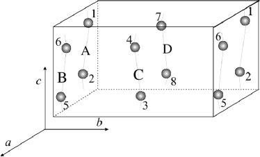
Figure 7: Unit cell of BaCu₂Si₂O₇. Notation of the ion positions and unequivalent chains.

In the above consideration we have described the observed frequency-field dependences of the antiferromagnetic resonance modes assuming that the transverse magnetic susceptibility is essentially anisotropic with respect to the orientation of the order parameter. The additional transitions occur in this model as a result of the competition between the loss in the anisotropy energy and of the gain in Zeeman energy, due to the increase of transverse magnetization at a rotation of the order parameter. For an ordinary antiferromagnet these terms become comparable at high magnetic fields, of the order of the exchange field. Hence, in order to explain the observed moderate values of the transition fields, one has to imply (see Eqns. (3)—(5)) that either the $B_{i}$ coefficients are unusually large, or the anisotropy parameters $a_{i}$ are particularly small.

The qualitatitive microscopic analysis given below demonstrates that the spin reduction affects differently anisotropy constants and the anisotropy of the transverse susceptibility and, therefore, is a likely reason of unusual spin-reorientation transitions. We start from the microscopic Hamiltonian and then proceed with a classical approximation, considering spins as vectors of length $S$. This classical approach cannot account for all possible effects of spin reduction, e.g. this consideration neglects the most probable anisotropy of the quantum spin fluctuations, which could be another reason for the anisotropy of the transverse susceptibility and contribute also to the induction of the described spin reorientation transitions. Our intention here is only to show qualitatively that effect of spin reduction is different for different terms in the energy even in classical approximation.

In the model described below we consider only in-chain Dzyaloshinskii-Moriya (DM) interaction and $g$-tensor anisotropy. Both of them originate from the relativistic spin-orbital interaction and are of the same order in spin-orbital coupling:Moriya $D/J\sim\delta g/g$. As before, we use Cartesian coordinates related to the orthorhombic unit cell: $x||a$, $y||b$, $z||c$.

As a first step, we consider the one-dimensional spin-chain running along $c$ axis. Note, that there are four inequivalent chains passing through the unit cell (see Figure 7). Magnetic ions within a chain are connected by the screw axis of symmetry $C_{2}^{\prime}$ aligned along the $c$ axis.

The in-chain Hamiltonian can be written as

$$\hat{\cal{H}}=\sum_{i}\left\{\bigl{(}\mathbf{\hat{\mathbf{S}}_{i}}\cdot\mathbf{\hat{\mathbf{S}}_{i+1}}\bigr{)}+\left(\mathbf{D_{i}}\cdot\bigl{[}\mathbf{\hat{\mathbf{S}}_{i}}\times\mathbf{\hat{\mathbf{S}}_{i+1}}\bigr{]}\right)+\mathbf{h}\widetilde{g_{i}}\hat{\mathbf{S}}_{i}\right\}$$ (20)

Here all interactions are normalized by the in-chain exchange integral, which is supposed to be antiferromagnetic. The magnetic field is normalised by the relation $\mathbf{h}=(\overline{g}\mu_{B}\mathbf{H}/J)$. The $g$-tensor is also normalised by the average $g$-factor: ($\widetilde{g}/\overline{g})\leftrightarrow\widetilde{g}$. Thus, for the renormalized $g$-tensor $Tr(\widetilde{g})=3$, and in the isotropic case $g_{\alpha\beta}=\delta_{\alpha\beta}$.

The screw axis puts constraints on the components of the Dzyaloshinskii-Moriya interaction vector $\mathbf{D}_{i}$ and on the components of the $g$-tensor $\widetilde{g_{i}}$; they can be written as a sum of staggered and uniform parts.

$$\mathbf{D}_{i} = (-1)^{i}\left(\begin{array}[]{c}\alpha\\ \beta\\ 0\end{array}\right)+\left(\begin{array}[]{c}0\\ 0\\ \gamma\end{array}\right)$$ (27)

$$\widetilde{g_{i}} = \left(\begin{array}[]{ccc}g_{xx}&g_{xy}&0\\ g_{xy}&g_{yy}&0\\ 0&0&g_{zz}\end{array}\right)+(-1)^{i}\left(\begin{array}[]{ccc}0&0&g_{xz}\\ 0&0&g_{yz}\\ g_{xz}&g_{yz}&0\end{array}\right)$$ (34)

The direction of the DM-vector is determined by the geometry of superexchange bonds: for the case of a simple copper-oxygen-copper superexchange path in BaCu₂Si₂O₇ it should be orthogonal to the plane of the copper-oxygen bonds. This orientation results in the relation of the DM vector components $|D_{x}|:|D_{y}|:|D_{z}|=1.70:1.00:0.16$. Here the crystal structure parameters of Ref. cryst-struct, are used. The above relation shows that the staggered component of DM vector dominates in the case of BaCu₂Si₂O₇.

The presence of the uniform component of the Dzyaloshinskii-Moriya interaction may cause an incommensurate helicoidal spin structure. In order to find the wavevector of the ground state we consider the Fourier-transformed spin vectors $\mathbf{S}_{i}=\sum_{\mathbf{k}}\mathbf{S}_{\mathbf{k}}e^{\imath(\mathbf{k}\cdot\mathbf{r}_{i})}$ and minimize numerically the Hamiltonian (20) over the wavevectors $\mathbf{k}$. Thus we have found that for a ratio between the uniform and staggered DM vector components less then 0.500, the commensurate state is favored. For the BaCu₂Si₂O₇ structure, the ratio of the uniform $z$-component of the DM vector to the staggered $xy$-component equals to 0.08, which certainly corresponds to the commensurate phase.

The commensurate state of a spin chain is a two-sublattice state, it may be described by the two orthogonal vectors $\mathbf{S}_{0}$ and $\mathbf{S}_{\pi}$. Spin vector at the $i$-th site of the chain is expressed via these Fourier components as $\mathbf{S}_{i}=\mathbf{S}_{0}+(-1)^{i}\mathbf{S}_{\pi}$. Energy of spin chain (per spin) can be written as

$$E=\mathbf{S}_{0}^{2}-\mathbf{S}_{\pi}^{2}+2\left(\mathbf{S_{0}}\cdot\bigl{[}\mathbf{S_{\pi}}\times\mathbf{D}\bigr{]}\right)+\mathbf{h}\widetilde{g_{u}}\mathbf{S}_{0}+\mathbf{h}\widetilde{g_{s}}\mathbf{S}_{\pi}$$ (35)

Here and further on, $\mathbf{D}$ denotes the staggered component of the DM vector only; $\widetilde{g_{u}}$ and $\widetilde{g_{s}}$ are uniform and staggered components of $g$-tensor, respectively.

The next step is to integrate over small component $\mathbf{S}_{0}$ to obtain the energy as a function of only the antiferromagnetic order parameter $\mathbf{l}=\mathbf{S}_{\pi}/|\mathbf{S}_{\pi}|$ and magnetic field. This integration is performed for $|\mathbf{S_{0}}|\ll S$. We keep all terms with field dependence not higher than $h^{2}$ and with coefficients not higher in spin-orbital coupling than $D^{2}$. The condition $|\mathbf{S_{0}}|\ll S$ effectively implies that our analysis is valid only in small fields $h\ll h_{E}=4S$.

The energy of the antiferromagnetically ordered chain per spin is:

$$E = -S^{2}-\frac{1}{8}[(\widetilde{g_{u}}\mathbf{h})\times\mathbf{l}]^{2}-\frac{S^{2}}{2}\bigl{[}\mathbf{l}\times\mathbf{D}\bigr{]}^{2}+$$ (36)

$$+\frac{1}{32}\bigl{[}\mathbf{h}\times\mathbf{l}\bigr{]}^{2}\bigl{[}\mathbf{D}\times\mathbf{l}\bigr{]}^{2}+\frac{1}{16}\left(\mathbf{h}\cdot\bigl{[}\mathbf{l}\times\mathbf{D}\bigr{]}\right)^{2}-$$

$$-\frac{1}{8}\left(\mathbf{h}\cdot\bigl{[}\mathbf{l}\times\mathbf{D}\bigr{]}\right)(\mathbf{h}\widetilde{g_{s}}\mathbf{l})-\frac{S}{2}(\widetilde{g_{u}}\mathbf{h})\cdot\bigl{[}\mathbf{l}\times\mathbf{D}\bigr{]}$$

Note, that in zero external field the order parameter $\mathbf{l}$ obeys the easy plane anisotropy and is confined to the plane, perpendicular to the staggered component of the Dzyaloshinskii-Moriya vector $\mathbf{D}$.

To find the total energy per unit cell it is necessary to sum contributions of all unequivalent chains taking into account inter-chain exchange interactions and symmetry-implied relations of Hamiltonian parameters in different chains (denoted as A, B, C and D):

$$\mathbf{D}_{A} = -\mathbf{D}_{B}$$ (37)

$$\mathbf{D}_{C} = -\mathbf{D}_{D}=\left(\begin{array}[]{c}\alpha_{A}\\ -\beta_{A}\\ 0\end{array}\right)$$ (41)

$$\widetilde{g_{u}}_{A} = \widetilde{g_{u}}_{B}$$ (42)

$$\widetilde{g_{s}}_{A} = -\widetilde{g_{s}}_{B}$$ (43)

$$\widetilde{g_{u}}_{C} = \widetilde{g_{u}}_{D}=\left(\begin{array}[]{ccc}g_{xx,A}&-g_{xy,A}&0\\ g_{xy,A}&g_{yy,A}&0\\ 0&0&g_{zz,A}\end{array}\right)$$ (47)

$$\widetilde{g_{s}}_{C} = -\widetilde{g_{s}}_{D}=\left(\begin{array}[]{ccc}0&0&-g_{xz,A}\\ 0&0&g_{yz,A}\\ -g_{xz,A}&g_{yz,A}&0\end{array}\right)$$ (51)

To simplify calculations we consider the exactly collinear state ($\mathbf{l}_{A}||\mathbf{l}_{B}||\mathbf{l}_{C}||\mathbf{l}_{D}$) with individual antiferromagnetic vectors corresponding to the order parameter observed in BaCu₂Si₂O₇ ($\mathbf{l}_{6}$ in terms of Ref.glazkov, ): $\mathbf{l}=\frac{1}{4}(\mathbf{l}_{A}+\mathbf{l}_{B}-\mathbf{l}_{C}-\mathbf{l}_{D})$. This order parameter corresponds to the minimum of the inter-chain exchange energy. By forcing all chains order parameters to be collinear we neglect a small contribution to the energy due to the weak canting of the antiferromagnetic structure, which is negligible, as checked by calculations.

As a result we find the following expression for the energy in the AFM state (per unit cell, additive constants omitted)

$$E = -\bigl{[}\mathbf{h}\times\mathbf{l}\bigr{]}^{2}+4S^{2}\alpha^{2}l_{x}^{2}+4S^{2}\beta^{2}l_{y}^{2}+$$ (52)

$$+2\left(\sum_{i=x,y,z}(g_{ii}-1)h_{i}l_{i}\right)\bigl{(}\mathbf{h}\cdot\mathbf{l}\bigr{)}+$$

$$+\left(\sum_{i=x,y,z}(g_{ii}-1)h_{i}l_{i}\right)^{2}+$$

$$+g_{xy}^{2}(h_{x}l_{y}+h_{y}l_{x})^{2}+\frac{1}{4}D^{2}\bigl{[}\mathbf{h}\times\mathbf{l}\bigr{]}^{2}-$$

$$-\frac{1}{4}\bigl{[}\mathbf{h}\times\mathbf{l}\bigr{]}^{2}(\alpha^{2}l_{x}^{2}+\beta^{2}l_{y}^{2})+\frac{1}{2}\alpha^{2}(l_{y}h_{z}-h_{y}l_{z})^{2}+$$

$$+\frac{1}{2}\beta^{2}(l_{x}h_{z}-l_{z}h_{x})^{2}+\alpha g_{yz}(h_{z}^{2}l_{y}^{2}-h_{y}^{2}l_{z}^{2})+$$

$$+\beta g_{xz}(h_{x}^{2}l_{z}^{2}-h_{z}^{2}l_{x}^{2})$$

Note, that the terms which are linear on the components of magnetic field $\mathbf{h}$ (see Eqn. (36)) exactly compensate each other. All four easy planes of magnetization of in-chain order parameters intersect along the $z$ axis, marking it as an easy axis of magnetization in agreement with experimental observations.

The energy in (52) reminds the phenomenologically written potential energy (1). It includes the field-independent anisotropy of the order parameter, exchange-relativistic terms similar to the terms with $\xi_{1,2}$ coefficients in (1), and the different relativistic terms quadratic over components of $\mathbf{l}$ and $\mathbf{h}$. The only essential difference is the presence of a term of fourth order in the components of $\mathbf{l}$ in Eqn. (52). We consider its effects below.

Now we point to the direct consequencies of Eqn. (52). Anisotropy terms are proportional to $S^{2}$, while field-dependent terms do not depend on $S$. Hence, in the antiferromagnet with strongly reduced sublattice magnetization anisotropy terms are strongly reduced in comparison with a conventional antiferromagnet. Direct comparison of Eqn. (1) and Eqn. (52) yields for the anisotropy constants $a_{1,2}=2S^{2}D_{x,y}^{2}/(g^{2}\mu_{B}^{2})$. Amplitude of the Dzyaloshinskii-Moriya interaction in the isostructural germanate BaCu₂Ge₂O₇ determined from the value of weak ferromagnetic moment is equal to 18K.bacugeo Taking for estimation $D_{\alpha}=10$K and assuming unreduced spin value $S=1/2$, we obtain for the value of anisotropy constant $a\sim 3000$kOe², which is about one order of magnitude larger then the values determined from the fit of AFMR frequency-field dependences (400 and 118 kOe²). This reduced anisotropy may explain why the spin-reorientations which should be observed in fields of the order of exchange field are shifted to lower fields.

Second, the exchange-relativistic terms $2(g_{ii}-1)h_{i}l_{i}\bigl{(}\mathbf{l}\cdot\mathbf{h}\bigr{)}$ are of the lower order in the spin-orbital coupling than other terms, quadratic in components of $\mathbf{l}$ and $\mathbf{h}$ . Indeed, $(g_{ii}-1)$ has the same order as $D$, while all the other coefficients are of the order of $D^{2}$. This means, in particular, that none of relativistic terms can be neglected in the Eqn. (1). Since exchange-relativistic terms $2(g_{ii}-1)h_{i}l_{i}\bigl{(}\mathbf{l}\cdot\mathbf{h}\bigr{)}$ have coefficients of lower order in the spin-orbital coupling, these terms could be taken into account even for a standard antiferromagnet: their effects become comparable with the anisotropy energy in the field $H_{g}\sim H_{A}^{1/4}H_{E}^{3/4}\ll H_{E}$.

The fourth order term in (52) does not affect the phenomenological analysis of the previous subsection. It can be decomposed to a sum of the second and fourth order terms $\Bigl{(}\mathbf{h}^{2}-\bigl{(}\mathbf{h}\cdot\mathbf{l}\bigr{)}^{2}\Bigr{)}\bigl{(}\alpha^{2}l_{x}^{2}+\beta^{2}l_{y}^{2}\bigr{)}$. The fourth order term written in this way does not affect static properties in the exact orientations of the magnetic field (it is always zero). Its dynamic effect is only small changes of the slope of AFMR branches, but the correction to the slope are dominated by the $g$-factor anisotropy producing terms of lower order in spin-orbital coupling ($D$ instead of $D^{2}$).

Finally, it is possible to calculate straightforwardly the magnetic susceptibility in low fields for several orientations of the magnetic field and of the order parameter. Taking an isotropic $g$-tensor and keeping in mind that from the exchange bond geometry $\alpha>\beta$, one can ascertain that $\chi(\mathbf{H}||z,\mathbf{l}||x)>\chi(\mathbf{H}||z,\mathbf{l}||y)$, $\chi(\mathbf{H}||y,\mathbf{l}||x)>\chi(\mathbf{H}||z,\mathbf{l}||z)$ and $\chi(\mathbf{H}||x,\mathbf{l}||y)>\chi(\mathbf{H}||x,\mathbf{l}||z)$. I.e. the anisotropy of the transverse magnetic susceptibility due to the Dzyaloshinskii-Moriya interaction favors the observed spin-reorientation transitions.

V Conclusions.

A detailed magnetic resonance study of the quasi-one-dimensional antiferromagnet BaCu₂Si₂O₇ is performed. We observed two low-energy spin-resonance modes at frequencies below 120GHz. Spin- reorientation transitions are marked by the softening of one of the resonance modes. Besides of the ordinary spin-flop transition a spin-reorientation transitions with spins rotating in the plane perpendicular to the magnetic field direction were identified.

The observed spin reorientations and magnetic resonance spectra in a wide frequency range are described quantitatively in a model taking into account the dependence of the transverse susceptibility on the direction of the order parameter. The role of this kind of anisotropy is shown to be enhanced in a quasi one-dimensional antiferromagnet due to the strong quantum reduction of the ordered spin component.

- (1) M. Kenzelmann, A. Zheludev, S. Raymond, E. Ressouche, T. Masuda, P. Böni, K. Kakurai, I. Tsukada, K. Uchinokura, and R. Coldea, Phys. Rev. B 64, 054422 (2001).
- (2) I. Tsukada, J. Takeya, T. Masuda and K. Uchinokura, Phys. Rev. Lett. 87, 127203 (2001).
- (3) A. Zheludev, E. Ressouche, I. Tsukada, T. Masuda and K. Uchinokura, Phys. Rev. B 65, 174416 (2002).
- (4) M. Poirier, M. Castonguay, A. Revcolevschi and G. Dhalenne, Phys. Rev. B 66, 054402 (2002).
- (5) M .D. Lumsden, B. C. Sales, D. Mandrus, S. E. Nagler, and J. R. Tompson, Phys.Rev.Letters 86, 159 (2001).
- (6) V. Glazkov and H.-A. Krug von Nidda, Phys.Rev.B 69, 212405 (2004).
- (7) H. Ohta, S. Okubo, K. Kawakami, D. Fukuoka, Y. Inagaki, T. Kunimoto, Z. Hiroi, J. Phys. Soc. Jpan., 72 Suppl. B pp. 26-35 (2003).
- (8) R. Hayn, V. A. Pashchenko, A. Stepanov, T. Masuda, and K. Uchinokura, Phys. Rev. B 66, 184414 (2002).
- (9) Juliana A. S. Oliveira, PhD thesis Ruprecht-Karls University, Heidelberg (1993)
- (10) T. Nagamiya, K. Yosida and R. Kubo, Advances in Physics 13, 1 (1955).
- (11) A. F. Andreev, V. I. Marchenko, Sov.Phys.Uspekhi 130,39 (1980).
- (12) V. V. Eremenko, V. M. Naumenko, V. V. Pishko, Yu. G. Pashkevich. Pisma v Zh. Eksp. Teor.Fiz 38, 97 (1983) [JETP Letters ].
- (13) T. Moriya, Phys. Rev. 120, 91 (1960).
- (14) I. Tsukada, J. Takeya, T. Masuda, and K. Uchinokura, Phys. Rev. B 62, R6061 (2000).