Statics and Dynamics of Strongly Charged Soft Matter

Abstract

Soft matter materials, such as polymers, membranes, proteins, are often electrically charged. This makes them water soluble, which is of great importance in technological application and a prerequisite for biological function. We discuss a few static and dynamic systems that are dominated by charge effects. One class comprises complexation between oppositely charged objects, for example the adsorption of charged ions or charged polymers on oppositely charged substrates of different geometry. Here the main questions are whether adsorption occurs and what the effective charge of the resulting complex is. We explicitly discuss the adsorption behavior of polyelectrolytes on substrates of planar, cylindrical and spherical geometry with specific reference to DNA adsorption on supported charged lipid layers, DNA adsorption on oppositely charged cylindrical dendro-polymers, and DNA binding on globular histone proteins, respectively. In all these systems salt plays an important role, and some of the important features can already be obtained on the linear Debye-Hückel level. The second class comprises effective interactions between similarly charged objects. Here the main theme is to understand the experimental finding that similarly and highly charged bodies attract each other in the presence of multi-valent counterions. This is demonstrated using field-theoretic arguments as well as Monte-Carlo simulations for the case of two homogeneously charged bodies. Realistic surfaces, on the other hand, are corrugated and also exhibit modulated charge distributions, which is important for static properties such as the counterion-density distribution, but has even more pronounced consequences for dynamic properties such as the counterion mobility. More pronounced dynamic effects are obtained with highly condensed charged systems in strong electric fields. Likewise, an electrostatically collapsed highly charged polymer is unfolded and oriented in strong electric fields. All charged systems occur in water, and water by itself is not a very well understood material. At the end of this review, we give a very brief and incomplete account of the behavior of water at planar surfaces. The coupling between water structure and charge effects is largely unexplored, and a few directions for future research are sketched. On an even more nanoscopic level, we demonstrate using ab-initio methods that specific interactions between oppositely charged groups (which occur when their electron orbitals start to overlap) are important and cause ion-specific effects that have recently moved into the focus of interest.

1 Introduction

Processes and structures involving electrostatic interactions are abundant in soft matter and play an important role in colloidal, polymeric, and biological systems[1, 2, 3, 4, 5, 6, 7, 8]. This is because charges tend to make objects soluble in water. Even the ubiquitous van-der-Waals or dispersion interactions are in fact due to locally fluctuating electric fields (or, equivalently, spontaneous polarization charges)[9]. Soft materials are easily deformed or rearranged by potentials comparable to thermal energy; examples include polymers, self-assembled membranes or micelles and complexes formed by the binding of oppositely charged macromolecular components. It becomes clear that interactions caused and mediated by permanent and induced charges constitute prominent factors determining the behavior and properties of soft matter at the mesoscopic scale, since they are strong enough to control and modify soft matter structures. We list three examples to demonstrate the diversity of phenomena we have in mind:

• Colloids that are dispersed in aqueous solvents experience mutual attractions due to van-der-Waals forces[9, 10] and additional solvent-structure-induced forces[11]. They thus tend to aggregate and form large agglomerates[12]. Large aggregates typically sediment, thereby destroying the dispersion. In colloidal science, this process is called coagulation or flocculation, depending on the strength and range of the inter-colloidal forces involved. In many industrial applications (for example dispersion paints, food emulsions such as mayonnaise or milk), stability of a dispersion is a desirable property, in other applications (such as sewage or waste-water treatment) it is not[13, 14]. One way to stabilize a colloidal dispersion against coagulation is to impart permanent charges to the colloids: Similarly charged particles typically repel each other such that van-der-Waals attraction (which is always stronger than electrostatic repulsion at small distances) cannot induce aggregation[10]. Every rule has an exception, and in this particular case it is an interesting exception: It has been found over the years that strongly charged colloids in certain cases attract strongly, which caused considerable confusion at first and is now quite well understood due to intense research over the last years (more of this in Section 3)[4, 5, 6, 7, 8]. A second method of stabilizing a colloidal dispersion is to graft polymers to the surface of the colloids. If the polymers are under good-solvent conditions, they will swell and inhibit close contacts between two colloids. For this task, charged polymers are ideal, since they swell a lot in water[15]. Many structures obtained with charged colloids bear resemblance with atomic structures, but occur on length and time scales that are much easier to observe experimentally. To some extent, colloidal systems have been used as models for ordering phenomena on the atomistic scale.

• Polymer science and technology have revolutionized the design, fabrication, and processing of modern materials and form an integral part of every-day life[16, 17, 18]. Classical polymer synthesis is based on hydro-carbon chemistry and thus leads to polymers which are typically insoluble in water. In the quest for cheap, environmentally friendly, and non-toxic materials, attention has shifted to charged polymers, so-called polyelectrolytes, since they are typically water-soluble[19, 20, 21]. The mechanism behind this water-solubility is connected with the translational entropy of mobile ions that are trapped in the polyelelctrolyte solution[22]. For some polyelectrolytes, the resulting affinity for water is so high that they are righteously called super-adsorbing polymers: They can bind amounts of water in multiple excess of their own weight[23]. This property is put to good use in many practical applications such as diapers.

• Human DNA, the storage medium of all genetic information, is a semiflexible biopolymer with a total length of roughly $2m$, bearing a total negative charge of about $10^{10}e$ (where $e$ denotes an elementary charge), which is contained inside the cell nucleus with a diameter of less than $10\mu m$. In addition to the task of confining such a large, strongly charged object in a very small compartment, the DNA is incessantly replicated, repaired, and transcribed, which seems to pose an unsurmountable DNA-packaging problem. Nature has solved this by an ingenious multi-hierarchical structure. On the lowest level, a short section of the DNA molecule, consisting of 146 base pairs (corresponding to a length of roughly $50nm$) is wrapped twice around a positively charged protein (the so-called histone). By this, the DNA is both compactified and partially neutralized. In experiments[24], it has been shown that a tightly wrapped state is only stable for intermediate, physiological salt concentrations. Since salt modulates the electrostatic interactions, it is suggested that electrostatics are responsible for this interesting behavior. Indeed, as is explained in Section 6, only at intermediate salt concentration is an optimal balance between electrostatic DNA–DNA repulsion (favoring a straight DNA conformation) and the DNA–histone attraction achieved. Similar complexes between charged spherical objects and oppositely charged polymers are also studied experimentally in the context of micelle-polymer[25, 26] and colloid-polymer[27, 28, 29, 30] interactions.

In these examples, electrostatic interactions dominate, they are responsible for the salient features and the characteristic properties and therefore have to be included in any theoretical description. This is the type of system we aim at in this review, and this is also the operational definition of a strongly charged system: a system where it makes sense to neglect other interactions than Coulombic in a first approximation (a more quantitative definition will be introduced in Section 3). Of course, the boundary to materials where other interactions come into play as well is diffuse: water structures at neutral and charged interfaces exhibit surprising properties and can often not be neglected, as is discussed in Section 10. Likewise, almost all phenomena involving charges in aqueous solution show a characteristic ion-specificity[31], namely a poorly understood dependence on the specific ion type present in the bulk, which is somehow related to the quantum-chemical properties of solvated ions (see Section11).

Our viewpoint is that it makes sense to use the whole scenario of simplified models theoretical physicists love and are used to, namely to treat charged macroions as smooth, featureless and homogeneously charged bodies, ions as point-like or (on a higher level) as charged spheres, and to replace water by a continuum medium. This was very successful in the past (as is reviewed in Sections 3 and 5-8) and there are many lessons still to be learned on this level. At the same time, many of the presently pressing experimental questions can only be answered if one leaves this level and treats water as a discrete solvent with the capability to rearrange at surfaces and close to charged particles and ions as complex objects that form weak bonds with other charges or water molecules. It is as yet not clear whether fundamental insight can be gained on this more microscopic level or whether one will be lost in the realm of particularities (Sections 10 and 11 give testimony of the problems one encounters when dealing with charges in the microscopic world). The hope would be that a coarse-grained formulation in terms of effective parameters will still be possible which would nevertheless encompass ion-specific and solvation effects.

2 Charges: Why and how

Almost any material acquires a surface charge when dipped into water. Permanent charges on single molecules, surfaces, or interfaces in aqueous media arise via two routes: Firstly, the substance can contain dissociable surface groups, which under suitable pH conditions may donate protons (in which case one speaks of acidic groups), thereby imparting negative charges to the surface, or accept protons (these are called basic groups) and thus produce positive charges on the surface (the pH is a logarithmic measure of the bulk proton concentration, as will be discussed at length in Section 9). What is the mechanism for this dissociation? Why should molecules fall apart spontaneously to produce charged parts and why do these oppositely charged pieces not bind together again? As an example, consider the ionisation of hydrogen, which requires the energy of $E_{ion}=13.6eV$ or (in units of the thermal energy at room temperatures) $E_{ion}\approx 500k_{B}T$. Clearly, this ionization process cannot be thermally activated at room temperatures. The situation is very different for chemical groups which have acidic character: Here the energy needed to remove a proton from the molecule in an aqueous environment is much smaller; to give a few examples, it is roughly $14k_{B}T$ for the carboxyl group in the reaction

$$RCOOH+H_{2}O\rightarrow RCOO^{-}+H_{3}O^{+}$$ (1)

and $9k_{B}T$ for the sulfonic group in the reaction

$$RSO_{3}H+H_{2}O\rightarrow RSO_{3}^{-}+H_{3}O^{+}.$$ (2)

The sulfonic group is therefore said to be a stronger acid than the carboxylic group. The dielectric properties of the surrounding water are very important in these reactions, as without water (i.e. in the gas phase) these reactions cost much more energy (see Section 11). Still, energy has to be paid in order to crack the acids, but again water properties come in: Since the concentration of water molecules in the condensed liquid state (about $55mol/l$) is much higher than of the other components, according to the law of mass action the equilibrium is shifted to the right side and charged groups do indeed occur frequently. The equilibrium between association and dissociation can be fine-tuned by temperature and the concentration of $H_{3}O^{+}$ ions in the solution (i.e. $pH$). The second mechanism for the permanent charging of surfaces involves small charged molecules, such as salt ions, which physically or chemically adsorb to a surface, thereby leading to an effective surface charge. In practice, one typically encounters a mixture of these two mechanisms, such that the effective charge of a surface is controlled by the distribution of acidic and basic surface groups, solution pH, and bulk concentration of charged solutes. Induced charges arise via the polarization of atoms, molecules, and macroscopic bodies[32]. For molecules that possess a permanent dipole moment (such as water), the macroscopic polarization contains a large contribution from the orientation of such molecular dipole moments. The interaction between spontaneous polarization charges gives rise to van-der-Waals forces, which act between all bodies and particles, regardless of whether they are charged, contain permanent dipole moments or not[10, 9].

The reduced electrostatic interaction between two spherically symmetric charges in vacuum (throughout this review, all energies are given in units of the thermal energy $k_{B}T$) can be written as $U(r)=Q_{1}Q_{2}v(r)$ where

$$v(r)=\frac{e^{2}}{4\pi\varepsilon_{0}k_{B}Tr}$$ (3)

is the Coulomb interaction between two elementary charges, $Q_{1}$ and $Q_{2}$ are the reduced charges in units of the elementary charge $e$, and $\varepsilon_{0}$ is the vacuum dielectric constant. The interaction only depends on the distance $r$ between the charges. Electrostatic interactions are additive, therefore the total electrostatic energy of a given distribution of charges results from adding up all pairwise interactions between charges according to Eq.(3). In principle, the equilibrium behavior of an ensemble of charged particles (e.g. a salt solution) follows from the partition function, i.e., the weighted sum over all different microscopic configurations, which —via the Boltzmann factor— depends on the electrostatic energy of each configuration. In practice, however, this route is complicated for several reasons:

i) The Coulomb interaction, Eq.(3), is very long-ranged, such that (even, and as turns out, especially for low densities) many particles are coupled due to their simultaneous electrostatic interactions. Electrostatic problems are therefore typically many-body problems. As is well known, even the problem of only three bodies interacting via gravitational potentials (which are analogous to Eq.(3) except that they are always attractive) defies closed-form solutions. To make the problem even worse, even if we consider only two charged particles, the problem effectively becomes a many-body problem, for the following two reasons:

ii) In almost all cases, charged objects are dissolved in water. As all molecules and atoms, water is polarizable and thus reacts to the presence of a charge with polarization charges. In addition, and this is a by far more important effect, water molecules carry a permanent dipole moment, and are thus partially oriented in the vicinity of charged objects. The polarization effect of the solvent can to a good approximation be taken into account by introducing a relative dielectric constant $\varepsilon$[32, 33, 34, 35]. Note that for water, $\varepsilon\approx 80$, so that electrostatic interactions are much weaker in water than in air (or some other low-dielectric solvent). The Coulomb potential now reads

$$v(r)=\frac{e^{2}}{4\pi\varepsilon_{0}\varepsilon k_{B}Tr}=\frac{\ell_{B}}{r}$$ (4)

and the Bjerrum length $\ell_{B}=1/(4\pi\varepsilon\varepsilon_{0}k_{B}T)$, which is a measure of the distance where the interaction is of thermal strength, has the value $\ell_{B}\approx 0.7nm$.

iii) In all biological and most industrial applications, water contains mobile salt ions. Salt ions of opposite charge are drawn to charged objects and form loosely bound counter-ion clouds and thus effectively reduce their charges; this process is called screening. The effect of charge screening is dramatically different from the presence of a polarizable environment. As has been shown by Debye and Hückel some 80 years ago[36], screening modifies the electrostatic interaction such that it falls off exponentially with distance.

The following points are important for the discussion in the subsequent sections: For each surface charge an oppositely charged counterion is released into the aqueous solution. These counterions form clouds that are loosely bound to the surface charges. The interactions between charged bodies and their electric properties itself (such as their electrophoretic mobilities in an electric driving field) are predominantly determined by the properties of these counterion clouds, and an understanding of the properties of charged bodies requires an understanding of the counterion clouds first. Highly and opppositely charged surfaces or particles with permanent charges typically have interaction potentials that are much stronger than thermal energy, one often obtains quasi-bound complexes which have to be dealt with in a very different way than the rather diffuse and highly fluctuating counterion distributions. Typically, charged soft matter (e.g. polymers, fluid membranes) is deformable and shows thermally excited shape fluctuations, and one is dealing with the intricate interplay of shape and counterion fluctuations. Electric fields are used in electrophoresis experiments to analyze and purify charged soft matter. The electric field sets charged ions and particles in motion and thus leads to dissipation of energy, one is facing a non-equilibrium situation. It also changes the equilibrium distribution functions, and can lead to non-equilibrium phase transitions, as will be shown towards the end of this review. Finally, oppositely charged chemical groups are often in intimate contact to each other, for example in situations when oppositely charged bodies are bound to each other. The boundary between chemical binding and salt bridging is diffuse, and quantum-mechanical effects which are caused by the overlap of electron orbitals give sizeable and very specific contributions to the effective interaction between charged groups. For a detailed understanding of the statistics and dynamics of charged soft matter, those quantum-mechanical effects in principle have to be taken into account.

3 Interactions between charged objects

3.1 Attraction between similarly charged plates: a puzzle?

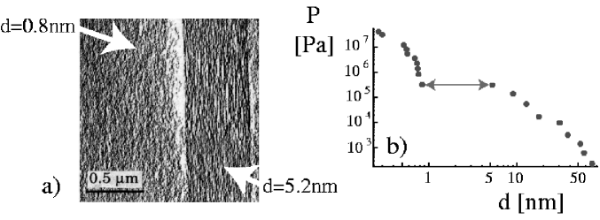
Figure 1: a) Cryo-electron-micograph of a membrane stack consisting of equal amounts of water and DDAB surfactant, frozen in from the equilibrated structure at room temperature, exhibiting macroscopic phase separation between two lamellar phases of different water content and thus different spacing between the bilayers (adapted from Ref.[39]). b) Osmotic pressure as a function of the water-layer thickness $d$. A pronounced plateau is apparent(adapted from Ref.[40]).

Experimentally, the interaction between charged planar objects can be very elegantly studied using a stack of charged, self-assembled membranes[37]-[43]. Such membranes spontaneously form in aqueous solution of charged amphiphilic molecules (lipids or surfactants) and consist of bilayers which are separated by water slabs of thickness $d$ (it is the same structure that forms an integral part of biological cell walls)[44]. Since the membranes are highly charged (they typically contain one surface charge per $0.6nm^{2}$ and thus belong to the most highly charged surfaces known), one would expect strong repulsion between them, or, which is equivalent, a strongly positive and monotonically decaying osmotic pressure in such a stack. In contrast, experiments using the cationic surfactant DDAB show that a mysterious attraction exists between the charged lamellae[39, 40]. This is seen in Fig.1a, where an electron-micrograph of a sample containing 50 % water and 50 % DDAB, rapidly frozen from the equilibrated structure at room temperature (and thus representative of the room-temperature situation) is shown. One can discern a two-phase coexistence between two macroscopic lamellar phases with different water-layer thicknesses $d$. In the corresponding pressure/surfactant concentration isotherm (obtained at room temperature) in Fig.1b the osmotic pressure shows a pronounced plateau as a function of the water-layer thickness, equivalent to macroscopic coexistence of two lamellar phases with different water content. Such phase coexistences are best known from non-ideal gases and result from an attraction between the gas molecules (compare the van-der-Waals equation of state). In the present case, it means that an attractive force acts between the highly charged membranes, strong enough to overcome the electrostatic repulsion between the charges on the membrane (note that the dispersion attraction is too weak by orders of magnitude to account for this attraction). This is quite surprising, and cannot be explained within classical theories (based on a mean-field description for the counterion distribution). Clearly, the real membrane system is quite complex and contains a number of effects that we will not consider (such as shape fluctuations, chemical structure of the surfactant heads, etc.). But we will demonstrate in the following that a simple argument for the counterion induced interaction between charged surfaces suffices to explain the observed miscibility gap in an almost quantitative fashion. This will lead us to a theoretical description of strongly coupled charged systems which complements the classical mean-field theory. In all the above-cited experiments on charged lamellar phases monovalent counterions were employed. We should add that a similar attraction is also seen with less strongly charged bilayer systems when the mono-valent counterions are replaced by divalent counterions[45, 46].

3.2 Counterions at a single charged plate

The experimentally observed attraction between similarly charged surfaces requires a deeper understanding of counterion layers at highly charged surfaces, we therefore start our discussion with a single, planar charged plate with counterions only (i.e. no additional salt ions). The Hamiltonian for a system of $N$ counterions of valence $q$, located at positions ${\bf r}_{i}$, close to a single oppositely charged planar wall of charge density $\sigma_{s}$ is (in units of $k_{B}T$) given by

$${\mathcal{H}}=\sum_{j=1}^{N-1}\sum_{k=j+1}^{N}\frac{q^{2}\ell_{B}}{|{\bf r}_{j}-{\bf r}_{k}|}+2\pi q\ell_{B}\sigma_{s}\sum^{N}_{j=1}{z}_{j},$$ (5)

where $\ell_{B}\equiv e^{2}/4\pi\varepsilon\varepsilon_{0}k_{B}T$ is the Bjerrum length ($e$ is the elementary charge, $\varepsilon$ is the relative dielectric constant). In water, one typically has $\ell_{B}\approx 0.7nm$. For the sake of simplicity, the dielectric constant is assumed to be homogeneous throughout the system, the plate is smooth, impenetrable to ions and homogeneously charged, and the counterions are assumed to be point-like. Still, the system is nontrivial and allows to understand the special features of strongly charged systems in a very lucid manner. The first term in Eq.(5) contains the Coulombic repulsion between all ions, the second term accounts for the electrostatic attraction to the wall (which is assumed to be of infinite lateral extent and located in the $z=0$ plane). The relevant length scale in the system is the Gouy-Chapman length, $\mu$, which is defined as the distance from the charged wall at which the potential energy of one isolated counterion equals the thermal energy $k_{B}T$. As will turn out later, it is a measure of the typical height of the counterion layer. From Equation (5) it can be read of to be

$$\mu=\frac{1}{2\pi q\ell_{B}\sigma_{s}}.$$ (6)

If one expresses all lengths in units of the Gouy-Chapman length and rescales them according to

$$\tilde{r}=r/\mu,$$ (7)

the Hamiltonian Equation (5) can be rewritten as

$${\mathcal{H}}=\sum_{j=1}^{N-1}\sum_{k=j+1}^{N}\frac{\Xi}{|\tilde{\bf r}_{j}-\tilde{\bf r}_{k}|}+\sum^{N}_{j=1}\tilde{z}_{j}.$$ (8)

Now the Hamiltonian only depends on a single parameter, the coupling parameter

$$\Xi=2\pi q^{3}\ell_{B}^{2}\sigma_{s}\sim\frac{q^{3}\sigma_{s}}{T^{2}},$$ (9)

which includes the effects of varying temperature $T$ (via the Bjerrum length $\ell_{B}$), surface charge density $\sigma_{s}$, and counterion valence $q$. The counterion valence enters the coupling parameter as a cube, showing that this is an experimental parameter which decisively controls the resultant behavior of the double layer (compare the experiments with charged lamellar systems where the counterion valency has been increased[45, 46]). Small values of $\Xi$ define the weak-coupling regime (where, as we will demonstrate later on, the mean-field Poisson-Boltzmann (PB) theory becomes valid), large values define the strong-coupling (SC) regime, where surface-adsorbed ions are strongly correlated[47, 48, 49]. This strong-coupling regime constitutes a sound physical limit with behavior very different from the PB limit, as can be shown rigorously using field-theoretic methods[50]-[54].

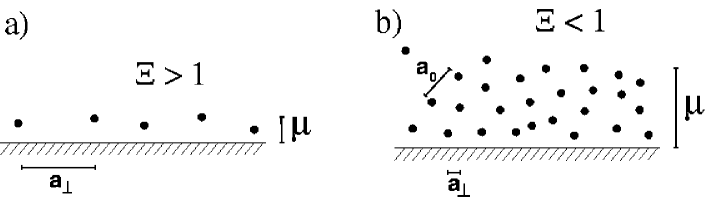
Figure 2: a) For large coupling parameter $\Xi>1$ the lateral distance between ions $a_{\perp}$ is larger than their average separation from the wall, proportional to the Gouy-Chapman length $\mu$. In rescaled units, this lateral distance reads $\tilde{a}_{\perp}=a_{\perp}/\mu=\sqrt{8\Xi}$. The layer is essentially flat, two-dimensional and strongly correlated. b) For $\Xi<1$, the lateral ion separation $a_{\perp}$ is smaller than the layer height $\mu$. Within the counter-ion layer, the inter-ionic distance $a_{0}$ scales as $\tilde{a}_{0}=a_{0}/\mu\sim\Xi^{1/3}$ and the ion-ion correlations are rather weak.

The mean lateral area per counter-ion is determined by the surface charge density and defines a length scale (which we associate with the lateral distance between ions), $a_{\perp}$, via the relation

$$\pi(a_{\perp}/2)^{2}=q/\sigma_{s}.$$ (10)

In rescaled units, this lateral distance reads

$$\tilde{a}_{\perp}=a_{\perp}/\mu=\sqrt{8\Xi}.$$ (11)

Since the height of the bound counterion cloud is unity in reduced units, it follows from equation (11) that for coupling parameters larger than unity, $\Xi>1$, the lateral distance between ions is larger than their separation from the wall and thus the layer is essentially flat and two-dimensional, as is shown schematically in Fig. 2a[47, 49]. For $\Xi<1$, on the other hand, the lateral ion separation $a_{\perp}$ is smaller than the layer height $\mu$, which means that within the counter-ion layer the ion-ion correlations should be rather 3D fluid-like, as depicted schematically in Fig. 2b. The two different limits are visualized in Figure 3, where we show snapshots of counterion distributions obtained in Monte-Carlo simulations for two different values of the coupling parameter, $\Xi=1,100$. For small $\Xi$, the ion distribution is indeed rather diffuse and disordered and mean-field theory should work, since each ion moves in a weakly varying potential due to the diffuse cloud of neighboring ions. For large $\Xi$, on the other hand, ion-ion distances are large compared to the distance from the wall; the ions form a flat layer on the charged wall. For large $\Xi$, the repulsion between condensed ions at a typical distance $a_{\perp}$, proportional to $\ell_{B}q^{2}/a_{\perp}$, is large compared with thermal energy, as can be seen from the fact that

$$\frac{\ell_{B}q^{2}}{a_{\perp}}\sim\sqrt{\Xi}\sim\frac{a_{\perp}}{\mu}.$$ (12)

The layer is thus flat and also strongly coupled[49]. As will be shown in Section 3.5, the counterion layer forms a crystal around $\Xi\approx 31000$[55], meaning that there is a wide range of coupling parameters, $1<\Xi<31000$, where the counterion layer is highly correlated but still liquid. Nevertheless, mean-field theory, which can pictorially be viewed as an approximation where one laterally smears out the counterion charge distribution, is expected to break down, at least for the system with $\Xi=100$; this is so because each ion moves, though confined by its immediate neighbors in the lateral directions, almost independently from the other ions along the vertical direction (which constitutes the soft mode). We stress that this continuous crossover from a three-dimensional, disordered counterion distribution for small $\Xi$, to a two-dimensional correlated counterion distribution for large values $\Xi$ (which will be discussed in more detail later on) is a pure consequence of scaling analysis; as the only input, it requires the rescaled counterion layer height to be of order unity, which is true irrespective of the precise value of $\Xi$ as will be demonstrated next.

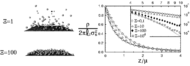
Figure 3: a) Snapshots of counterion distributions at a charged surface for two different values of the coupling parameter, showing a rather diffuse distribution for small $\Xi$ and a flat quasi-two dimensional layer for large $\Xi$. b) Numerically determined counterion density profiles (data points) as a function of the distance from the surface for different values of the coupling parameter $\Xi$ in comparison with the asymptotic predictions in the mean-field (solid curve) and strong-coupling (broken line) limits (adapted from Ref.[50]).

Using Monte-Carlo simulation techniques, we have obtained counterion density profiles by averaging over statistically sampled counterion configurations for different values of $\Xi$. Since the surface charge density is homogeneous, the counterion density profile $\rho(z)$ only depends on the distance from the wall, $z$. The counterions exactly neutralize the surface charges, the integral over the counterion density profile is therefore given by (in unrescaled units) $\int_{0}^{\infty}{\rm d}z\;\rho(z)=\sigma_{s}/q$. Using the rescaled distance coordinate $\tilde{z}=z/\mu$, the integral gives $\int_{0}^{\infty}{\rm d}\tilde{z}\;\rho(\tilde{z})=2\pi\ell_{B}\sigma_{s}^{2}$, which suggests to define the rescaled density profile as

$$\tilde{\rho}(\tilde{z})=\frac{\rho(\tilde{z})}{2\pi\ell_{B}\sigma_{s}^{2}}$$ (13)

which, via the condition of electroneutrality, is normalized to unity,

$$\int_{0}^{\infty}{\rm d}\tilde{z}\;\tilde{\rho}(\tilde{z})=1.$$ (14)

In Figure 3b we show rescaled counterion density profiles obtained using Monte Carlo simulations for various values of the coupling parameter $\Xi=0.1$, $10$, $100$ and $10^{4}$. One notes that all profiles saturate at a rescaled density of unity at the charged wall. This is in accord with the contact-value theorem, which states that the counterion density at the wall is —for the case of a single homogeneously charged wall— exactly given by $\rho(0)=2\pi\ell_{B}\sigma_{s}^{2}$, or, in rescaled units,

$$\tilde{\rho}(0)=1$$ (15)

(incidentally in agreement with the Poisson-Boltzmann prediction)[56, 57, 58]. The contact value theorem Eq.(15) follows from the requirement of vanishing net force acting on the wall, which means that the osmotic pressure, in units of $k_{B}T$ given by the counterion density at the wall, $P_{os}=\rho(0)$, has to cancel the electrostatic attractive force between wall and counterion layer, which is given by $P_{el}=-2\pi\ell_{B}\sigma_{s}^{2}$, i.e. $P_{os}+P_{el}=0$, from which Eq. (15) directly follows. Given the two constraints on the rescaled density profile, namely being normalized to unity and reaching a contact density of unity at the wall, Equations (14) and (15), it is clear that the profiles in the units chosen by us have to be quite similar to each other even for vastly different coupling parameters, as indeed observed in Figure 3b. Also, it is a rather trivial consequence of both constraints that the typical decay length of the profiles is always given by unity in rescaled units (though, strictly speaking, the first moment $\langle\tilde{z}\rangle$ of the density distribution diverges logarithmically within PB theory). Still, the asymptotic predictions for vanishing coupling constant ($\Xi\rightarrow 0$, PB theory, solid line in Figure 3b) and diverging coupling constant ($\Xi\rightarrow\infty$, SC theory, broken line) are as different as they can be from a functional point of view, while still obeying the constraints mentioned above, as we will now recapitulate.

At low coupling, the counterion density distribution is well described by the Poisson-Boltzmann (PB) theory, which predicts an algebraically decaying profile[59, 60, 61]

$$\tilde{\rho}_{\rm PB}(\tilde{z})=\frac{1}{\left(1+\tilde{z}\right)^{2}},$$ (16)

while in the opposite limit of high coupling the strong coupling (SC) theory, predicting an exponentially decaying profile[50, 52]

$$\tilde{\rho}_{\rm SC}(\tilde{z})=\exp\bigr{(}-\tilde{z}\bigr{)},$$ (17)

becomes asymptotically exact. An exponential density profile (although with a different pre-factor) has also been obtained by Shklovskii[49] using a heuristic model for a highly charged surface, where counterions bound to the wall are in chemical equilibrium with free counterions. The intuitive explanation for the exponential density profile Equation (17) uses the fact that for large values of the coupling constant, the lateral distance between counterions is large and therefore a counterion mostly interacts with the charged plate and experiences the bare linear wall potential, the second term in Equation (8), with only small corrections due to other ions. The single-ion distribution function follows by exponentiating the linear wall potential, similar to the derivation of the barometric height formula for the atmospheric density, and in agreement with the result in Equation (17). It is important to note, though, that Equation (17) has been obtained as the leading term in a systematic field-theoretic derivation which also gives correction terms[52] which in turn have been favorably compared with simulation results[53]. As can be seen from Figure 3b, the PB density profile Equation (16) is only realized for $\Xi<1$, while the strong-coupling profile Equation (17) is indeed the asymptotic solution and agrees with simulation results for $\Xi>10^{4}$ over the distance range considered in the simulations. In fact, there is a crossover between the two asymptotic theories which is distance dependent[52, 53], as we will briefly discuss now.

In the strong coupling limit $\Xi>1$ an expansion of all observables in inverse powers of $\Xi$ can be set up that has much in common with a virial expansion[52, 53]. The density distribution can thus be written as

$$\tilde{\rho}(\tilde{z})=\tilde{\rho}_{SC}(\tilde{z})+\frac{1}{\Xi}\tilde{\rho}_{SC}^{(1)}(\tilde{z})+{\cal O}(\Xi^{-2})$$ (18)

with the leading correction to the asymptotic strong-coupling profile given by[52]

$$\tilde{\rho}_{SC}^{(1)}(\tilde{z})={\rm e}^{-\tilde{z}}\left(\frac{\tilde{z}^{2}}{2}-\tilde{z}\right).$$ (19)

A systematic estimate of the limits of accuracy of the asymptotic SC theory is furnished by comparing the leading and next-leading contributions, Eqs.(17) and (19), which enter the systematic SC-expansion of the counter-ion density Eq.(18). This limit of applicability turns out to be distance-dependent. For large separations $\tilde{z}\gg 1$ the SC theory should be valid for

$$\Xi>\tilde{z}^{2}.$$ (20)

Using the relation between the lateral distance between counter-ions, $\tilde{a}_{\perp}$, and the coupling parameter, Eq.(11), the latter threshold can be transformed into $\tilde{a}_{\perp}>\tilde{z}$ or $a_{\perp}>z$. This means that the SC approach should be valid as long as one considers distances from the wall, $z$, smaller than the average lateral distance between counter-ions, $a_{\perp}$. This is in accord with the intuitive expectation since the bare wall potential prevails for these distances.

In the small-coupling regime, $\Xi<1$, a similar expansion can be performed using the field-theoretic tool of a loop-expansion[62, 63, 52]. We obtain for the density profile the expansion in powers of the coupling parameter

$$\tilde{\rho}(\tilde{\bf r})=\tilde{\rho}_{PB}(\tilde{\bf r})+\Xi\tilde{\rho}_{PB}^{(1)}(\tilde{\bf r})+{\cal O}(\Xi^{2}).$$ (21)

This shows directly that the saddle-point (or mean-field) method, which yields the first (leading) term, is good when the coupling parameter $\Xi$ is small. For large values of $\Xi$, higher-order terms become important. For large separations from the wall, the asymptotic behavior has been determined explicitly as[62]

$$\tilde{\rho}_{PB}^{(1)}(\tilde{z})\simeq-\frac{\ln\tilde{z}}{\tilde{z}^{3}}.$$ (22)

The correction in Eq.(22) decays faster than the leading term in Eq.(16). By comparing the two expressions, one obtains that for large separations from the plate, $\tilde{z}\gg 1$, the PB prediction for the density, Eq.(16), should be valid for coupling parameters

$$\Xi<\frac{\tilde{z}}{\ln(\tilde{z})}.$$ (23)

This shows that it does not make sense to talk about the accuracy of the PB or SC approach per se for a given coupling parameter $\Xi$. Rather, from Eq.(23) it is seen that the PB solution becomes more accurate as one moves further away from the plate. Conversely, from Eq.(20) the SC solution becomes more accurate as one moves closer to the plate. By comparing Eqs. (20) and (23) one realizes that for large distances from the wall (or for large coupling strengths), a gap appears over the distance range

$$\sqrt{\Xi}<\tilde{z}<\Xi$$ (24)

where neither of the asymptotic theories is applicable. This gap widens as the coupling strength increases and can be interpreted as a distance range where the density distribution is neither described by the SC result $\tilde{\rho}\simeq e^{-\tilde{z}}$, see Eq.(17), nor the PB result, Eq.(16), which for large separations reads $\tilde{\rho}\simeq\tilde{z}^{-2}$. That an intermediate scaling range has to exist already follows from the fact that the asymptotic density profiles cross only once at a rescaled distance from the plate of the order of unity. In order to connect the SC and PB profiles continuously at much larger distances, one needs an intermediate distance range where the density decays slower than the inverse square with distance. Some ideas on how to understand and analytically describe this intermediate regime have been brought forward in Refs.[49, 52] In a number of recently published papers counterion density profiles were calculated for intermediate coupling parameter using various approximate theories and successfully compared with numerical data[64, 65, 66].

In summary, the strong-coupling theory is a theory that becomes asymptotically exact in the opposite limit when the mean-field or Poisson-Boltzmann theory is valid. The two theories therefore describe the two extreme situations, as can be seen most clearly in Figure 3. Experimentally, a coupling parameter $\Xi=100$, which is already quite close to the strong-coupling limit, is reached with divalent ions for a surface charged density $\sigma_{s}\approx 3.9nm^{-2}$, which is feasible with compressed charged monolayers, and with trivalent counter ions for $\sigma_{s}\approx 1.2nm^{-2}$, which is a typical value. The strong-coupling limit is therefore experimentally accessible and not only interesting from a fundamental point of view.

3.3 Charged plate in the presence of salt

The case of counterions at a wall is particularly simple, since the two length scales in the problem, namely the Gouy-Chapman length, $\mu$, and the mean-lateral distance between charges, $a_{\perp}$, can be combined into a single parameter according to $\Xi\sim(a_{\perp}/\mu)^{2}$. Experimentally, one is always dealing with aqueous solutions at finite salt concentration (and if it was only for ions due to the auto-dissociation of water, which gives rise to an ionic concentration of at least $10^{-7}$ mol/l and thus to a screening length of the order of a micrometer), so we have to have a look at how our arguments in the preceding section are modified in the presence of salt. Salt adds an additional length scale, namely the mean distance between salt ions in the bulk, see Figure 4, which we denote by $a_{s}$ and which is related to the salt concentration $c_{s}$ via $c_{s}\sim a_{s}^{-3}$. In principle, if the bulk contains oppositely charged ions, one also needs to give the ions a finite diameter $a$ to prevent them from collapsing into each other; however, in order to concentrate on the essentials, we will largely neglect the finite ion diameter in this Section. Thus we confine ourselves to three length scales, $\mu$, $a_{\perp}$, and $a_{s}$, that can be combined into two unitless parameters which fully define the problem. The actual physics, however, is quite rich, since from the three geometric length scales we define in Fig. 4, one can derive two additional length scales which play an important role, namely the screening length $\kappa^{-1}$ defined by $\kappa^{2}=8\pi\ell_{B}q^{2}c_{s}$, and the length at which two ions interact with thermal energy, $q^{2}\ell_{B}$.

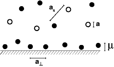
Figure 4: Schematic view of the relevant length scales for a charged wall in the presence of salt. The lateral distance between counterions in a neutralizing layer at the surface is denoted by $a_{\perp}$. The Gouy-Chapman length $\mu$ is the height of the counterion layer, and $a_{s}$ is the distance between salt ions in the bulk. Finally, the ion diameter is denoted by $a$. In the picture we chose $a_{\perp}>\mu$, equivalent to $\Xi>1$, meaning that we have a strong-coupling situation. We also chose $a_{s}>a_{\perp}$, which together with $\Xi>1$ means that the screening length $\kappa^{-1}$ satisfies $\kappa^{-1}>\mu$ and thus the counterion height is indeed given by the Gouy Chapman length.

Within mean-field, i.e. the Poisson-Boltzmann theory[59, 60, 61], the electrostatic potential $\psi(z)$ at a charged wall decays as $qe\psi(z)/k_{B}T=2\ln[(1-\gamma e^{-z\kappa})/(1+\gamma e^{-z\kappa})]$. The counter and coion density distributions at a charged wall follow within mean-field as

$$\rho^{+}_{PB}=c_{s}^{2}/\rho^{-}_{PB}=c_{s}e^{-qe\psi(z)/k_{B}T}=c_{s}\left(\frac{1+\gamma e^{-z\kappa}}{1-\gamma e^{-z\kappa}}\right)^{2}$$ (25)

where the constant $\gamma$ is determined by the equation

$$2\gamma/(1-\gamma^{2})=1/(\kappa\mu).$$ (26)

It is seen that the screening length gives the scale over which the ionic charge distribution decays towards the bulk value as one moves far away from the charged wall; in other words, the screening length is the correlation length of the salt solution.

In the following we will discuss various crossover boundaries for the system under investigation, which will eventually be summed up in a scaling diagram.

i) In the Debye-Hückel (DH) limit defined by

$$\kappa^{-1}<\mu$$ (27)

the screening length is smaller than the Gouy Chapman length; the charged surface perturbs the ionic densities only slightly, the mean-field equations can be linearized and the linear superposition principle for densities and potentials is valid. Eq.(26) is solved by $\gamma\simeq 1/(2\mu\kappa)$ and the potential is $qe\psi(z)/k_{B}T\simeq 2e^{-z\kappa}/(\mu\kappa)$ and the ion densities follow as $\rho^{\pm}_{PB}=c_{s}(1\pm 2e^{-\kappa z}/(\mu\kappa))$. When inequality Eq.(27) is not satisified, i.e. when the DH approximation is not valid, the algebraic density profile Eq.(16) is realized for the counterions at distances smaller than the screening length.

ii) If the interaction between salt ions at their mean separation $a_{s}$ is larger than thermal energy, we have a strongly coupled salt solution and mean-field theory breaks down, even in the bulk and in the absence of a charged surface. This condition reads $\ell_{B}q^{2}/a_{s}>1$ and can be reexpressed as

$$\Xi>(\kappa\mu)^{-1}.$$ (28)

In practice, an effective mean-field theory can be defined where the screening length is renormalized from its bare value[69]. Such a modified DH theory with renormalized screening length we denote by DH^∗. Since the intermediate distance range, where the counterion density profile is neither described by SC nor PB, is given by $\sqrt{\Xi}<\tilde{z}<\Xi$, Eq.(24), it follows that when Eq.(28) holds, the counterion density profile at large distances $\tilde{z}>\Xi$ can be described by a linear DH* theory since the non-linear PB regime is preempted by the intermediate regime where neither SC nor PB works.

iii) When the screening length becomes smaller than $a_{\perp}$, we expect the intermediate distance range, which is expected for the range ${\tilde{a}}_{\perp}\sim\sqrt{\Xi}<\tilde{z}<\Xi$, to disappear. The condition $\kappa^{-1}<a_{\perp}$ is equivalent to

$$\Xi>(\kappa\mu)^{-2}.$$ (29)

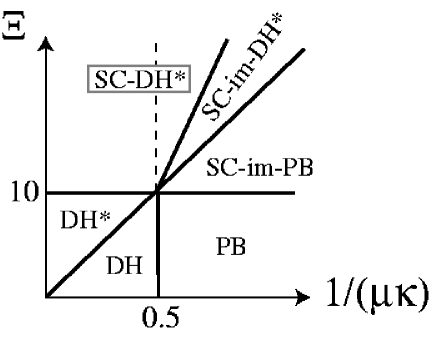
Figure 5: Scaling diagram for the behavior of a salt solution at a charged surface as a function of coupling parameter $\Xi$ and ratio of screening length $\kappa^{-1}$ and Gouy-Chapman length $\mu$. Axes are logarithmic, meaning that power laws are straight lines. Effects of bulk correlations between salt ions and correlations between counterions at the surface are included. The various phases and scaling boundaries are explained in the text. The crossover between PB and DH is located at $1/\mu\kappa\approx 1/2$, since there the electrostatic potential at the surface is roughly unity in terms of the thermal energy, i.e., $qe\psi/k_{B}T\approx 1$; for monovalent ions this corresponds to $\psi=25mV$.

All three scaling boundarie Eqs.(27- 29) are represented in Fig. 5, where we chose as axes the coupling parameter $\Xi$ and the ratio of screening length and Gouy-Chapman length, $\kappa^{-1}/\mu$. The horizontal line in addition denotes the boundary between weak coupling and strong coupling regimes, which roughly occurs at $\Xi\approx 10$, see Fig. 3b. In the scaling regime ’PB’ the ordinary Poisson-Boltzmann theory is valid and the ion densities are correctly described by Eq.(25). In the Debye-Hückel regime denoted by ’DH’, the linearized version of PB is sufficient. In the phase ’DH*’ the salt is strongly coupled, and ion pairs proliferate. This can be taken care of by a renormalized screening length. Now we move to the phases for strong coupling constant $\Xi>1$, where things are more interesting but also less certain. In the phase ’SC-im-PB’ the ion density profile exhibits three different scaling ranges: for $\tilde{z}<\sqrt{\Xi}$ the strong-coupling profile is realized, $\sqrt{\Xi}<\tilde{z}<\Xi$ defines the intermediate range (where predictions based on a Gaussian theory have been advanced in Ref.[52]), and for $\Xi<\tilde{z}$ the Poisson Boltzmann profile is valid (note that the PB profile itself is subdivided into a nonlinear range $\Xi<\tilde{z}<1/(\kappa\mu)$ and a linear DH range $1/(\kappa\mu)<\tilde{z}$). In the ’SC-im-DH*’ phase the non-linear PB range has disappeared, and finally, in the ’SC-DH*’ phase the intermediate range has been swallowed up by the DH* scaling range. The SC-DH* phase is curious, since the counterion density profile is expected to show a crossover between two exponential decays governed by two different decay lengths, namely the Gouy-Chapman length (for small distances) and the screening length (for large distances). It is itself subdivided by a broken line into two subregimes. The right regime is more interesting, since here the charged wall induces counterion concentrations much higher than the bulk concentration and thus a quite visible effect (as will be shown shortly in simulation data). The crossover between the two exponential decays, however, will be hard to observe in practice.

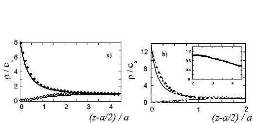
Figure 6: Counterion (filled symbols) and coion (open symbols) density profiles obtained within simulations as a function of the distance from the charged wall divided by the ion diameter, $(z-a/2)/a$. a) PB regime with weak coupling $\Xi=2.3$ where PB profiles, Eqs.(25), solid lines, are accurate. The Coulomb interaction between two ions at contact is $\zeta=q^{2}\ell_{B}/a=1.75$ and the rescaled screening length is $\kappa^{-1}/\mu=1.26$. The Gouy-Chapman length in units of the ion diameter is $\mu/a=0.758$. b) Strong coupling regime ’SC-im-DH*’ with $\Xi=18.9$ where PB (solid lines) breaks down. Coulomb strength is $q^{2}\ell_{B}/a=5$ and the rescaled screening length is $\kappa^{-1}/\mu=1.71$ and $\mu/a=0.265$. The broken line is the salt-modified strong-coupling profile for the counterions, Eq.(30). The inset shows a gradual density depression at the uncharged upper system boundary, which is caused by correlation effects (see discussion in text).

In Fig.6 we show counterion and coion density profiles at a charged wall as obtained in Brownian dynamics simulations[70]. The profile in Fig.6a is obtained for a coupling parameter $\Xi=2.3$ and a rescaled screening length $\kappa^{-1}/\mu=1.26$. According to our scaling arguments advanced above, this system belongs to the Poisson-Boltzmann regime, and indeed the PB profiles Eq.(25), solid lines, match the simulation results very nicely. The data in Fig.6b are obtained for $\Xi=18.9$ and $\kappa^{-1}/\mu=1.71$. Since the crossover in $\Xi$ occurs for $\Xi\approx 10$, the system belongs to the SC regime and indeed the PB prediction (solid lines) performs poorly. In order to compare the data with the strong-coupling profile, which was derived in the counterion-only-case, we have to use additional information. First of all, the counterion profile saturates at a finite value far away from the surface which is given by the bulk salt concentration. Secondly, the ion density at the wall still obeys the contact-value theorem, which is slightly modified in the presence of salt: The net pressure acting on the wall is not zero, as with counterions only, compare Eq. (15), but equals the bulk osmotic pressure $P_{bulk}$. In the limit of a weakly coupled salt solution (i.e. for a small bulk-plasma parameter or for $\Xi<1/\mu\kappa$), the bulk osmotic pressure is that of an ideal gas, $P_{bulk}=2c_{s}$. Neglecting also correlation effects at the surface, which are similar to the Onsager-Samarras effect[71], the pressure acting on the surface equals the sum of the surface osmotic pressure, $P_{os}=\rho^{+}(0)+\rho^{-}(0)$, proportional to the surface ion densities, and the electrostatic double layer attraction attraction $P_{el}=-2\pi\ell_{B}\sigma_{s}^{2}$, compare our discussion after Eq. (15). Equating surface and bulk pressures, $P_{bulk}=P_{os}+P_{el}$, we obtain $2c_{s}=\rho^{+}(0)+\rho^{-}(0)-2\pi\ell_{B}\sigma_{s}^{2}$. Using that for a highly charged surface the coion surface density $\rho^{-}(0)$ vanishes, we obtain $\rho^{+}(0)\approx 2c_{s}+2\pi\ell_{B}\sigma_{s}^{2}$. The simplest functional satisfying the surface and the bulk constraints, and which decays according to the SC prediction Eq.(17), is

$$\frac{\rho_{SC}^{+}(\tilde{z})}{c_{s}}=1+(1+4\mu^{-2}\kappa^{-2})e^{-\tilde{z}}$$ (30)

which is shown in Fig.6b as a broken line and describes the data quite well. The coion distribution is quite featureless close to the wall and equally well described by the PB or by a modified SC expression.

A pronounced density depression of both coions and counterions is seen in the inset of Fig.6b at the uncharged boundary surface located at $z/a=5$. This is analogous to the aforementioned Onsager-Samarras effect according to which the ions in an electrolyte solution are repelled from a low-dielectric substrate[71, 72]. In the present case the dielectric constant is uniform, but still the ions are repelled from the bounding surface since the effective polarizability of the salt solution is higher than that of the half-space devoid of ions[73].

After having discussed the counterion distribution at a single charged wall, it is now time to go on to the experimentally relevant case of two charged walls.

3.4 Counterions between two charged plates

A great deal of work has been devoted in the past twenty years to understanding the interaction between two double layers. Specifically, it has been known for some time that two similarly and strongly charged plates can attract each other in the presence of multivalent counterions or even with monovalent counterions when the surface charge density is extremely high. This has been seen in Monte Carlo simulations[74, 75], observed experimentally with the surface force apparatus[76] and also deduced from the phase diagrams of charged lamellar systems[45, 46, 40], as has been discussed in Section 3.1. A similar attraction is theoretically predicted for highly charged cylinders[77]-[89], flexible polymers[90] and spheres as well[91]-[101] and is thus by no means confined to the planar geometry. Experimentally, a long-ranged attraction has also been seen for charged spherical colloids confined by walls[102, 103, 104, 105], although it has been shown in the mean time that for some setups the effect can be caused by hydrodynamic artifacts. For other setups the long-ranged interaction persists. It was very recently argued that optical artifacts caused by the imaging process can lead to minute distortions in the particle distances as obtained by digital video microscopy. Those distortions in turn result in an apparent minimum in the interaction energy[106]. The general occurrence of like-charge attraction is quite relevant concerning the stability of colloidal solutions, since it means that the stabilization of colloids with charges can fail if the surfaces are too highly charged. Such behavior strongly contradicts the Poisson-Boltzmann theory, which predicts that the electrostatic interaction between similarly charged surfaces is always repulsive[61]. Most theoretical approaches (beyond PB) tried to include the correlations between counterions, which were thought to be the reason for the discrepancy between the mean-field and the experimental/simulation results and which are neglected on the mean-field level[107, 2]. The first theoretical approach that demonstrated the existence of attraction between equally charged plates (with electrostatic origin) is due to Kjellander and Marčelja[108], who used a sophisticated integral-equation theory (with HNC closure) and obtained results that compared very well with simulations[74, 108, 109]. Also perturbative expansions around the PB solution[110, 111, 62] and density-functional theory[112, 113] were used, and predicted as well the existence of an attractive interaction. For plates far away from each other, i.e., at distances such that the two double layers weakly overlap, the attractive force was obtained within the approximation of two-dimensional counterion layers by including in-plane Gaussian fluctuations[114, 115, 116, 117] and, more recently, plasmon fluctuations at zero temperature[118] and at non-zero temperatures[119]. Fluctuation-induced interactions between macroscopic objects constitute a quite general phenomenon, which is present whenever objects couple to a fluctuating background field[120], giving rise to a wide range of interesting phenomena including colloidal flocculation in binary mixtures[11].

The rescaled pressure $\tilde{P}$ between two plates in the presence of counterions only is given by the contact value theorem

$$\tilde{P}=\frac{P}{2\pi\ell_{B}\sigma_{s}^{2}}=\frac{\rho(0)}{2\pi\ell_{B}\sigma_{s}^{2}}-1,$$ (31)

which relates the pressure in units of $k_{B}T$, $P$, acting on one wall to the counterion density at that wall, $\rho(0)$ (which in a simulation can be extracted via a suitable extrapolation scheme). As has been discussed before, the first term on the right-hand side is the osmotic pressure due to counterion confinement, the second term is the double layer attraction between the counter-ions and the charged plates. This theorem can be formulated in different ways and is exact[56, 57, 58]. Clearly, the pressure depends on the rescaled distance $\tilde{d}=d/\mu$ between the two walls.

The mean-field (Poisson-Boltzmann) prediction for the pressure follows from equation (31) as

$$\tilde{P}_{\rm PB}(\tilde{d})=\Lambda$$ (32)

where $\Lambda$ is determined by the transcendental equation[121]

$$\frac{1}{\Lambda^{1/2}}=\tan\biggl{(}\frac{\tilde{d}}{2}\Lambda^{1/2}\biggr{)}$$ (33)

which is solved by

$$\tilde{P}_{\rm PB}(\tilde{d})=\left\{\begin{array}[]{llll}&2\tilde{d}^{-1}-1/3&{\rm for}&\tilde{d}\ll 1\\ &\pi^{2}\tilde{d}^{-2}&{\rm for}&\tilde{d}\gg 1.\\ \end{array}\right.$$ (34)

As is well-known, the PB pressure is always repulsive[61].

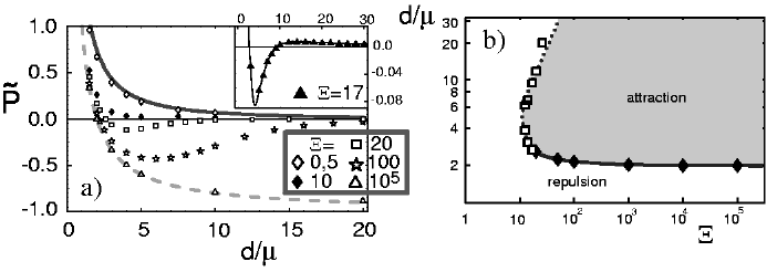
Figure 7: a) Simulation results for the rescaled pressure $\tilde{P}\equiv P/2\pi\ell_{B}\sigma_{s}^{2}$ as a function of the plate separation $\tilde{d}=d/\mu$ for different values of the coupling parameter $\Xi$. The solid line denotes the PB prediction Equation (32) and the broken line the SC prediction Equation (35). The error bars are smaller than the symbols. Note that for large enough distances, all MC data exhibit positive pressures. b) The global behavior of the inter-wall pressure as obtained from the simulations, showing the region where the pressure between two charged walls is negative (attractive) and where the pressure is positive (repulsive). The dividing line denotes a line of vanishing pressure. The filled diamonds (and full line) denote the thermodynamically stable distance between the plates. The open squares correspond to a metastable local minimum (lower branch) and a maximum (upper branch) in the free energy. For couplings $\Xi>\Xi_{n}\approx 12$, there is a range in $\tilde{d}$ where the pressure is negative (attraction). At $\Xi=\Xi_{u}\approx 17$ a first-order unbinding transition occurs (as follows from the Maxwell construction).

Within the strong-coupling theory, the leading result for the pressure is[51, 52]

$$\tilde{P}_{\rm SC}(\tilde{d})=\frac{2}{\tilde{d}}-1$$ (35)

and will be derived using simple arguments below. While the PB theory predicts that the pressure is always positive (only repulsion), the SC theory gives attraction between the plates for $\tilde{d}>2$ (negative pressure) and thus predicts a bound state (free energy minimum) at a distance $\tilde{d}^{*}=2$. In analogy to the strong-coupling result for the counterion density profile at a single charged wall, and as is explained in detail in Ref.[52], the leading term of the SC expansion for the pressure, equation (35), is the first virial term and thus follows from the partition function of a single counterion sandwiched between two charged plates.

Since the lateral distance between two counterions is of the order of $\tilde{a}_{\perp}\simeq\sqrt{\Xi}$ in rescaled coordinates, see Eq.(11), and since we expect the SC theory to be a good approximation as long as the lateral distance between counterions is larger than the plate distance, i.e. for $\tilde{a}_{\perp}>\tilde{d}$, the SC result should be valid for

$$\Xi\gg\tilde{d}^{2}$$ (36)

(this argument can be substantiated by a Ginzburg argument based on comparing different orders in the SC perturbation expansion[52]). The SC theory at the same time predicts a bound state at a rescaled plate separation $\tilde{d}^{*}=2$. This prediction for the bound state is thus within the domain of validity of the SC theory for coupling constants $\Xi>4$. One could therefore argue that the mechanism of the attraction between similarly charged bodies is contained in the SC theory. To gain intuitive insight into this mechanism, we reconsider the partition function of a single counterion sandwiched between two charged plates which we now explicitly evaluate. Denoting the distance between the counterion and the plates (of area $A$) as $x$ and $d-x$, respectively, we obtain for the electrostatic interaction between the ion and the plates (note that all energies and forces are given in units of $k_{B}T$) for $d\ll\sqrt{A}$ the results $W_{1}=2\pi\ell_{B}q\sigma_{s}x$ and $W_{2}=2\pi\ell_{B}q\sigma_{s}(d-x)$, respectively, as follows from the potential of an infinite charged wall and omitting constant terms. The sum of the two interactions is $W_{1+2}=W_{1}+W_{2}=2\pi\ell_{B}q\sigma_{s}d$, which shows that i) no pressure is acting on the counter-ion since the forces exerted by the two plates exactly cancel and ii) that the counter-ion mediates an effective attraction between the two plates. The interaction between the two plates is proportional to the total charge on one plate, $A\sigma_{s}$, and for $d\ll\sqrt{A}$ given by $W_{12}=-2\pi A\ell_{B}\sigma_{s}^{2}d$. Since the system is electro-neutral, $q=2A\sigma_{s}$, the total energy is $W=W_{12}+W_{1}+W_{2}=2\pi A\ell_{B}\sigma_{s}^{2}d$, leading to an electrostatic pressure $P_{el}=-\partial(W/A)/\partial d=-2\pi\ell_{B}\sigma_{s}^{2}$ per unit area. The two plates attract each other! The osmotic pressure due to counter-ion confinement is $P_{os}=1/Ad=2\sigma_{s}/qd$. The total pressure is given by the sum $P_{\rm SC}=P_{el}+P_{os}$ and reads in rescaled units $\tilde{P}_{\rm SC}=2/\tilde{d}-1$ and thus agrees exactly with the result in Equation (35). The equilibrium plate separation is characterized by zero total pressure, $P_{\rm SC}=P_{el}+P_{os}=0$, leading to an equilibrium plate separation $d^{*}=1/\pi\ell_{B}q\sigma_{s}$, or, in rescaled units, $\tilde{d}^{*}=2$.

We collect the simulation results, as well as the asymptotic strong-coupling and Poisson-Boltzmann predictions in Figure 7a, where the pressure as a function of the distance between the charged walls is plotted for different values of the coupling. For a small coupling $\Xi=0.5$, PB (solid line), Equation (32), describes very well the MC results, while at very high coupling ($\Xi=10^{5}$) the SC theory (broken line), Equation (35), gives the correct prediction. Intermediate values of the coupling lead to values of the pressure that are bounded by the two asymptotic predictions, similarly to our findings for the single charged wall in the preceding section.

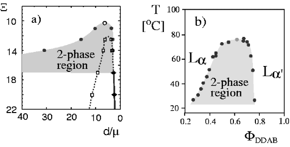
Figure 8: a) The same theoretical phase diagram as in Figure 7b, but enlarged around the region where the first-order unbinding transition occurs. The circles denote the binodal, determined according to the Maxwell construction, the open squares and filled diamonds are the points where the pressure is zero, corresponding to extrema of the free energy. At a coupling $\Xi=\Xi_{u}\approx 17$ a discontinuous unbinding transition occurs as one comes from higher $\Xi$ (correspondingly, one branch of the binodal moves to infinity as one comes from lower $\Xi$). Notice that a critical point is present at $\Xi=\Xi_{c}\approx 10.25$ (denoted by an open circle). The pressure is strictly positive for $\Xi<\Xi_{n}\approx 12$. The full and broken lines are guides to the eye. b) Experimentally determined binodal for a two component mixture of the cationic surfactant DDAB and water (reproduced after [39]).

We summarize the behavior of the pressure in the phase diagram Figure 7b, which shows the region of negative (attractive) pressure, separated from the region of positive (repulsive) pressure by a line on which the pressure is zero. This line can correspond to a thermodynamically stable, metastable, or instable state, as will be discussed in detail now. For couplings larger than $\Xi=\Xi_{n}\simeq 12$, there is a range of $\tilde{d}$ within which the pressure is negative and the two plates attract each other. The boundary between attraction and repulsion in Figure 7b is given by the points where the pressure is zero: the filled diamonds (connected by a solid line which serves as a guide to the eyes) correspond to thermodynamically stable bound states (absolute minima of the free energy at finite $\tilde{d}$), while the open squares (connected by a broken line) are local, metastable minima (lower branch) and maxima (upper branch) of the free energy. At a coupling $\Xi=\Xi_{u}\simeq 17$ a first-order unbinding transition occurs, where the free energy has two minima of equal depth, one at finite separation $\tilde{d}\simeq 3$ and the other at infinite separation $\tilde{d}=\infty$. Below this value of the coupling the absolute minimum of the free energy is at infinite plate separation, i.e., the thermodynamically stable state of the system is the unbound state, above this value, the thermodynamically stable state exhibits a finite value of the separation and is denoted by the solid line. We note that we determine the free energies from our data by integration of the pressure curve from infinite distance to a finite distance value. In the limit of large values of $\Xi$, the lower zero-pressure branch saturates at $\tilde{d}\approx 2$, in agreement with the asymptotic result of the SC theory.

The upper branch of the zero-pressure line can be estimated by field-theoretic methods: Within a loop expansion, the pressure is expanded in powers of the coupling parameter $\Xi$ according to

$$\tilde{P}=\tilde{P}_{PB}+\Xi\tilde{P}_{PB}^{(1)}+{\cal O}(\Xi^{2}).$$ (37)

The zero-loop prediction for the pressure follows from PB theory and is given in Eq.(34). The one-loop correction to the pressure has been calculated by Attard et al.[110] and by Podgornik[111] and is in reduced units given by

$$\tilde{P}_{PB}^{(1)}(\tilde{d})=\left\{\begin{array}[]{llll}&-2\tilde{d}^{-1}&{\rm for}&\tilde{d}\ll 1\\ &-\pi^{2}\tilde{d}^{-3}\ln\tilde{d}&{\rm for}&\tilde{d}\gg 1.\\ \end{array}\right.$$ (38)

The correction to the asymptotic PB result is attractive. By equating the two orders for large distances $\tilde{d}$ one obtains an estimate for the zero pressure line as

$$\Xi\simeq\tilde{d}/\ln(\tilde{d})$$ (39)

which agrees almost quantitatively with the numerical results in Figure 7b. However, one has to meet this result with all due suspicion and it receives credibility only due to the good agreement with the numerics, since the onset of attraction at the same time signals the break-down of the loop-expansion.

Experimentally, the solid line in Figure 7b describes the distance between charged plates in the thermodynamic ensemble when the external pressure is zero (this corresponds to the case where a lamellar phase is in equilibrium with excess water). If the plate-distance is controlled by some pressure acting on the system (which is relevant to the experimental situation where the total water content of a lamellar phase is fixed), the system exhibits a critical point and a binodal where two lamellar states with different spacings coexist thermodynamically. This is shown in Figure 8a, where in addition to the boundary between negative and positive pressures (shown as a broken and solid line) we also show the binodal, which has been numerically determined for a finite set of coupling constants (circles) and which corresponds to the boundary of the shaded region for values of coupling constant $\Xi<\Xi_{u}\approx 17$. The binodal corresponds to coexisting states, which are located through a Maxwell construction. This is demonstrated in Figure 9, where we schematically show the free energy and the corresponding inter-plate pressure for four different representative values of the coupling constant $\Xi$. The binodal exhibits a critical point (denoted by an open circle) at a coupling constant $\Xi_{c}\approx 10.25$ and at a plate separation $\tilde{d}\approx 6$. For smaller coupling constants, $\Xi<\Xi_{c}$ the pressure is strictly positive and decays monotonically. In the coupling constant range $\Xi_{c}<\Xi<\Xi_{n}\approx 12$ the thermodynamically coexisting states can be located using the Maxwell construction for the pressure profile (i.e. by enforcing the areas above and below the horizontal line in Fig. 9 to be the same) or for the free energy profile by the equivalent common-tangent construction (see Fig. 9; note that in this coupling range the free energy decays monotonically and the pressure is thus strictly positive). In the coupling constant range $\Xi_{n}<\Xi<\Xi_{u}\approx 17$ the pressure is negative for a range of distances limited by the open squares in Figure 8a. It is important to note that the pressure becomes positive for large distances, which reflects the fact that the mean-field theory becomes valid at large distances between the plates[52]. As the coupling constant increases, the binodal branch at large distances moves out to infinity. For the pressure data for $\Xi=\Xi_{c}=17$, which are shown in the inset in Figure 7a, the Maxwell construction leads to a coexisting state at infinite separation, which demarks the unbinding transition. From our arguments given above, the unbinding transition is a quite generic feature, caused by the fact that PB becomes valid and thus the pressure becomes repulsive at large separations. The ratio of the unbinding and the critical coupling is $\Xi_{u}/\Xi_{c}\approx 1.7$, leading to a temperature ratio of roughly $T_{c}/T_{u}\approx 1.3$.

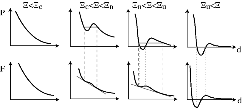
Figure 9: Schematic scenario for the evolution of the interplate pressure $P$ and the free energy $F$ as the coupling constant increases. The straight lines visualize the Maxwell construction for the pressure profile (top row) and the equivalent common-tangent construction for the free-energy profile (bottom row). The broken lines denote the thermodynamically coexisting state (i.e. points on the binodal) while the dotted lines denote states with vanishing pressure. The mechanism for the unbinding transition at a coupling constant $\Xi_{u}\approx 17$ is the repulsion (positive pressure) which is always observed at large distances.

In Figure 8b we reproduce the binodal of the cationic surfactant system DDAB (which also contains only counterions since salt has been carefully removed from the system)[40]. The general shape of the experimental binodal qualitatively agrees with the theoretical one in Figure 8a. It is interesting to note that for this experimental system, the critical point roughly occurs at a temperature of $T_{c}=75^{o}C$ or $348K$, which points (using the above estimate $T_{c}/T_{u}\approx 1.3$) to an unbinding transition of $T_{u}=268K$ or $-5^{o}C$, a little bit below freezing. The binodal in the experimental phase diagram somewhat follows the predicted unbinding behavior, since the binodal branch of the dilute lamellar phase indeed moves progressively to the left as the temperature is decreased[39, 40]. The critical surface charge density for monovalent counterions and at room temperature follows from our estimate $\Xi_{c}\approx 10$ to be equivalent to one surface charge per area 30 Ų. The membrane charge density in the above mentioned experiments is between 60 Ų and 70 Ų and therefore differs by a factor of two. Our comment about the ratio of the critical and unbinding temperatures therefore has to be taken as a rough estimate. The deviations might be caused by effects associated with dielectric boundaries and inhomogeneous surface charge distributions (which are both not included in our simple model) and which are likely to shift the critical point to larger values of the area per surface group. The distance between the charged surfaces at the critical point is given by $\tilde{d}_{c}\approx 6$, which for monovalent counterions is equivalent to roughly $0.6nm$. We note that the finite size of the ions is not really important for average-size ions, since the spacing $d$ used in our simulations corresponds to the vertical height available for the ionic centers. In other words, $d$ denotes the difference between the distance between the plate surfaces and the ionic diameters. Adding an ionic diameter of roughly $0.3nm$ to the theoretically predicted plate distance at criticality, one arrives at a plate separation of roughly $0.9nm$ which is indeed very close to what is seen experimentally.

3.5 Wigner crystallization

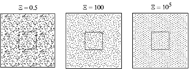
Figure 10: Top-view snapshots of counterions between two plates at separation $\tilde{d}=2$ for coupling parameters $\Xi=0.5$ and $N=150$ particles, showing only weak lateral correlations, $\Xi=100$ and $N=100$, showing short-ranged correlations, and $\Xi=10^{5}$ and $N=100$, exhibiting crystalline order, indicative of Wigner crystallization. The central square is the actual simulation box, the outer square visualizes the first shell of periodic neighbors.

Recently, there has been an active discussion about the significance of Wigner crystallization for the behavior of strongly charged matter such as the attraction between similarly charged plates[47, 49]. A two-dimensional one-component plasma is known to crystallize for a value of the plasma parameter $\Gamma\approx 125$[55]. From the definition of the two-dimensional plasma parameter[55], $\Gamma=\ell_{B}q^{2}/(q/\pi\sigma_{s})^{1/2}$, we obtain the relation $\Xi=2\Gamma^{2}$. This leads to a crystallization threshold (in units of our coupling parameter) of $\Xi\approx 31000$. For the system with two charged plates the crystallization is in the limit $\tilde{d}\rightarrow 0$ predicted to occur at $\Xi\simeq 15600$. In Figure 10 we show top-view snapshots for ions sandwiched between two plates, obtained within the Monte-Carlo simulations for $\Xi=0.5$, $\Xi=100$ and $\Xi=10^{5}$ at fixed inter-plate distance $\tilde{d}=2$. In agreement with the estimated Wigner crystallization threshold, $\Xi\simeq 15600$, the snapshots for $\Xi=0.5$ and $\Xi=100$ show liquid behavior, while the snapshot for $\Xi=10^{5}$ exhibits crystalline order. Since the experimentally relevant attraction occurs for values $\Xi<100$, it seems that Wigner crystallization is not connected or responsible for the attraction between similarly charged plates[7]. On the other hand, treating the strongly correlated liquid layer of counter-ions like a Wigner crystal is in many cases a reasonable approximation[49].

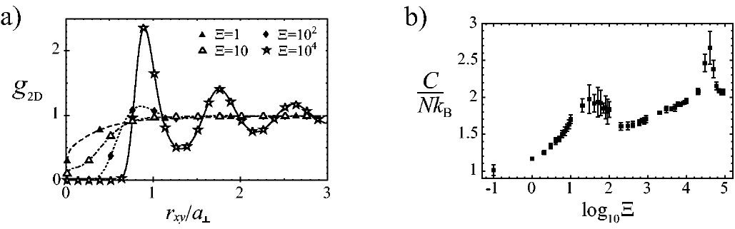
Figure 11: a) The two-dimensional pair distribution function of counterions at a single charged planar wall plotted as a function of the lateral distance $r_{xy}$ between counterions, obtained by averaging over the height z. Coupling parameters are $\Xi=1$ (filled triangles), $\Xi=10$ (open triangles), $\Xi=100$ (filled diamonds) and $\Xi=10^{4}$ (open stars). The lateral distance is rescaled by the scale $a_{\perp}=2\sqrt{q/(\pi\sigma_{s})}$. b) Excess heat capacity as a function of the coupling parameter. The number of counterions is N = 100 in a periodic square simulation box. The broad hump at intermediate coupling $10<\Xi<100$ reflects the structural change in the counterionic layer due to increasing correlations between counterions. At a coupling strength $\Xi\approx 31000$ the counterion layer crystallizes, as indicated by a pronounced peak in the heat capacity. Reproduced after [8].

To gain more quantitative information on the correlations in the counterion layer, we present results for the lateral two-point correlation function $g_{2D}$ at a single charged plate. Physically, $g_{2D}$ gives the normalized probability of finding two counterions at a certain lateral distance from each other. The Monte-Carlo results for this quantity are shown in Fig.11. For small coupling parameter, $\Xi=1$, filled triangles, there is only a very short-range depletion zone at small separations between counterions. A pronounced correlation hole is created for coupling parameters $10<\Xi<100$, where the distribution function vanishes over a finite range at small inter-particle separations. For larger coupling strengths, the correlation hole becomes more pronounced and is followed by an oscillatory behavior in the pair distribution function, $\Xi=10^{4}$, open stars. This indicates a liquid-like order in the counterionic structure in agreement with qualitative considerations in the preceding Sections. Note that the distance coordinate in Fig. 11a is rescaled by $a_{\perp}=2\sqrt{q/(\pi\sigma_{s})}$ as defined in Eq.(10). The location of the first peak of $g_{2D}$ for $\Xi=10^{4}$ appears at a distance of $r_{xy}/a_{\perp}\approx 0.9$. In a perfect hexagonal crystal, the peak is expected to occur at $r_{xy}/a_{\perp}=\sqrt{\pi/(2\sqrt{3})}\approx 0.95$, and in a perfect square crystal at $r_{xy}/a_{\perp}=\sqrt{\pi}/2\approx 0.89$. The crystallization in fact occurs at even larger coupling parameters, which can best be derived from the behavior of the heat capacity as a function of the coupling parameter $\Xi$. In Fig. 11b, the simulated excess heat capacity of the counterion-wall system (obtained by omitting the trivial kinetic energy contribution $3k_{B}/2$) is shown for various coupling parameters. The crystallization of counterions at the wall is reflected by a pronounced peak at large coupling parameters about $\Xi\approx 31000$, in good agreement with our estimate based on the 2D one-component plasma. The characteristic properties of the crystallization transition in the counterion-wall system are yet to be specified, which requires a detailed finite-size scaling analysis in the vicinity of the transition point. Another interesting behavior is observed in Fig. 11b at the range of coupling parameters $10<\Xi<100$, where the heat capacity exhibits a broad hump. This hump probably does not represent a phase transition[122], but is most likely associated with the formation of the correlation hole around counterions and the structural changes in the counterionic layer from three-dimensional at low couplings to quasi-2D at large couplings. In the region between the hump and the crystallization peak, for $200<\Xi<10^{4}$, the heat capacity is found to increase almost logarithmically with $\Xi$. The reason for this behavior is at present not clear.

The results in this section demonstrate that the Wigner crystallization transition, which has been studied extensively for a two-dimensional system of charged particles, also exists for a $2\frac{1}{2}$-dimensional system where the counterions are confined to one half space but attracted to a charged surface. This is a non-trivial result, and for the system of counterions sandwiched between two plates one expects interesting phase transitions between different crystal structures as the plate distance is varied and becomes of the order of the lateral distance between ions.

3.6 The zero-temperature limit

A word is in order on the connection of our strong-coupling theory to zero-temperature arguments for the pressure between charged surfaces which involve two mutually interacting Wigner lattices[47] and which were extended by including plasmon fluctuations at zero temperature[118] and at non-zero temperatures[119]. Is the SC theory in fact a zero-temperature limit? No, it is not, as can be seen from the asymptotically limiting pressure in Eq.(35): the first term is the confinement entropy of counterions, which clearly only exists at finite temperatures. Is the zero-temperature contained in the SC theory and can it be derived from it? Only partially: At zero temperature, the coupling constant tends to infinity, but on the other hand the Gouy-Chapman length (which sets the spatial scale) tends to zero, and thus all rescaled lengths blow up. Coming back to the pressure in Eq.(35), this means that the first, entropic term disappears and only the second, energetic term remains. This is in exact accord with the predictions of the zero-temperature Wigner-lattice theory for small plate separation[47]. For plate separations larger than the lateral ion separation, the Wigner-lattice theory predicts an exponential decay of the attraction, which however is not contained within SC theory since this is precisely the distance where SC starts to break down and an infinite resummation of all terms in the perturbation series would be needed. To make things more transparent, let us construct from the two parameters used for the two-plate system so far, $\Xi$ and $\tilde{d}$, which both depend on temperature, a parameter that does not depend on temperature: it is given by $\hat{d}=\tilde{d}/\Xi^{1/2}\sim d/a_{\perp}$ and thus is a purely geometric parameter describing the ratio of the distance between the plates to the lateral distance between ions. Sending $\Xi\rightarrow\infty$ at fixed $\hat{d}$ is the zero-temperature limit and corresponds to finding the ground state of a counterion arrangement at a fixed aspect ratio of the counterion-plate unit cell. The condition for validity of SC theory, Eq.(36), translates into $\hat{d}<1$, while from Eq.(39) the PB theory follows to be accurate for $\hat{d}>\Xi^{1/2}$ (which coincides with the upper branch of the zero-pressure curve). The lower branch of the zero-pressure line, Eq.(35), is given by $\hat{d}\sim\Xi^{-1/2}$. These scaling predictions are assembled in Fig. 12, where the zero-pressure lines are drawn as dotted lines and the limits of validity as solid lines. For large $\Xi^{-1}$ a regime appears where both regimes of validity overlap, as was discussed in Ref.[52], for small $\Xi^{-1}$ a large gap appears where non of the asymptotic PB and SC theories is valid. The zero-temperature limit is obtained for $\Xi^{-1}\rightarrow 0$ in this diagram and thus complements the PB and SC theories in that limit.

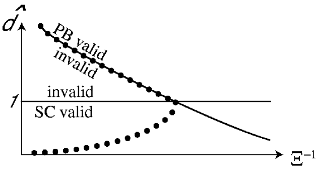
Figure 12: Schematic phase diagram for counterions between two plates as a function of the inverse coupling parameter $\Xi^{-1}\sim T^{2}/\sigma_{s}q^{3}$ and the temperature independent rescaled plate distance $\hat{d}=d/a_{\perp}$ where $a_{\perp}$ is the lateral distance between counterions. Shown are the rescaled conditions for validity of SC theory, Eq.(36), $\hat{d}<1$, validity of PB theory, Eq.(39), $\hat{d}>\Xi^{1/2}$, (which coincides with the upper branch of the zero-pressure curve, dotted line) and the lower branch of the zero-pressure line, Eq.(35), $\hat{d}\sim\Xi^{-1/2}$, dotted line. The zero temperature-limit corresponds to the limit $\Xi^{-1}\rightarrow 0$.

4 Charged structured surfaces

In the previous section we looked at the somewhat artificial model where the charged surface is smooth and homogeneously charged, and where the counterions are pointlike and thus only interact via Coulomb interactions. In reality, even an atomically flat surface exhibits some degree of corrugation, and counterions have a finite extent and thus experience some type of excluded-volume interaction.

In this section we consider a two-dimensional layer of $N$ charged spheres of valency $q$ and diameter $a$ (at $z=0$), together with $N$ oppositely charged counterions of the same valency and diameter, which are confined to the upper half space ($z>0$) in a cubic simulation box of length $D$, see Fig.13a. The number density of surface ions is $\rho_{s}=N/D^{2}$. The other important parameter is $\zeta=q^{2}\ell_{B}/a$ which measures the ratio of the Coulomb interaction and the thermal energy at the minimal inter-ionic distance $a$. Collapse of counterions and surface ions is prevented by a truncated Lennard-Jones term acting between all particles.

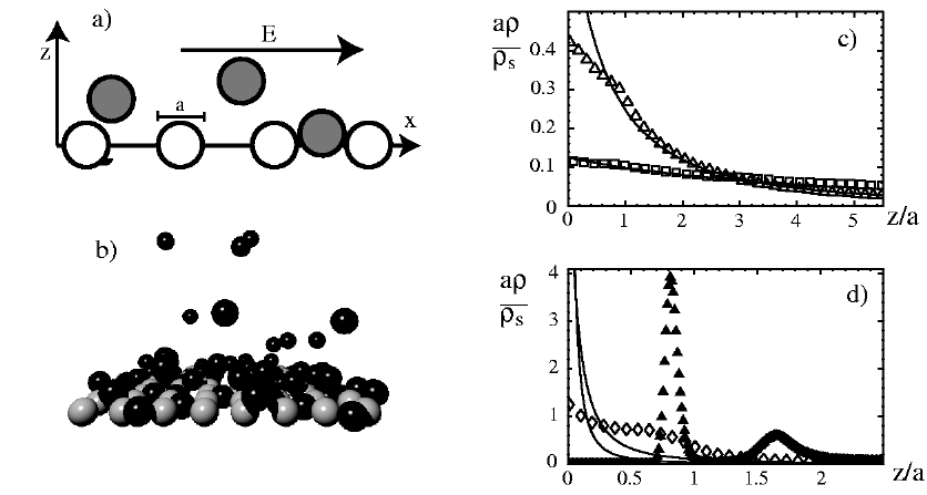
Figure 13: a) In the simulations a two-dimensional layer of fixed surface ions is in contact with oppositely charged counterions of the same diameter $a$ and valency $q$. b) Snapshot of an ion configuration for a surface density $\rho_{s}a^{2}=0.5$ and Coulomb parameter $\zeta=q^{2}\ell_{b}/a=2.5$. c) Laterally averaged counterion-density profiles for Coulomb coupling $\zeta=2.5$ as a function of the rescaled distance from the surface (surface ions are fixed on a square lattice). Shown are results for surface ion densities $\rho_{s}a^{2}=0.0079$ (open squares), $\rho_{s}a^{2}=0.05$ (open triangles), d) $\rho_{s}a^{2}=0.5$ (open diamonds) and $\rho_{s}a^{2}=2$ (filled triangles) together with the mean-field predictions for the laterally homogeneous case (solid lines).

The model we consider includes the combined effects of discrete surface charges, surface corrugations, and counterion excluded volume[123], which are all neglected in the classical mean-field approaches but have been considered quite recently[54, 124, 125, 91, 126, 127, 128, 129, 130, 131, 132, 133]. We employ Brownian-dynamics simulations where the velocity of all particles follows from the position Langevin equation. The proper canonical distribution functions are obtained by adding a suitably chosen Gaussian noise force acting on all particles and expectation values are obtained by averaging particle trajectories over time. In Fig.13b we show a snap shot of the counterion-configuration obtained during a simulation. In Fig.13c and d we show laterally averaged counterion density profiles for fixed Coulomb strength $\zeta=2.5$ and various surface ion densities. This Coulomb strength corresponds to a distance of closest approach between ions of 3 Å  which is a quite realistic value for normal ions. We also show the mean-field (MF) prediction for the laterally homogeneous case, Eq.(16), which reads in normalized form $a\rho(z)/\rho_{s}=\mu^{-1}/(1+z/\mu)^{2}$. As before, the Gouy-Chapman length $\mu=a/(2\pi\zeta a^{2}\rho_{s})$ is a measure of the decay length of the profiles. For small surface-ion densities, Fig.13c, the measured profiles agree quite well with the MF predictions, as expected, since the Gouy-Chapman length is larger than the lateral surface-ion separation and the charge modulation and hard-core repulsion matter little. However, even for the smallest density considered (open squares) there are some deviations in the distance range $z/a<1$ which we attribute to the hard-core repulsion between surface ions and counterions. For the larger surface densities in Fig.13d the deviations become more pronounced (simply shifting the MF profiles does not lead to satisfactory agreement). For $\rho_{s}a^{2}=0.5$ (open diamonds) some counterions still reach the surface at $z=0$, but the profile is considerably shifted to larger values of $z$ due to the impenetrability of surface ions and counterions. Finally, for $\rho_{s}a^{2}=2$ (filled triangles) the surface ions form an impenetrable but highly corrugated layer, and the counterion profile is shifted almost by an ion diameter outwards (and a second layer of counterions forms). These results remind us that in experimental systems a number of effects are present which make comparison with theories based on laterally homogeneous charge distributions difficult. As a side remark, the coupling constant $\Xi=2\pi\rho_{s}a^{2}\zeta^{2}$ (which measures deviations from MF theory due to fluctuations and correlations, see previous section) is for the data in Fig.13d in a range where deviations from MF theory are becoming noticeable for the smeared-out case[50]; for $\rho_{s}a^{2}=2$ one finds $\Xi\approx 75$ which means that Poisson-Boltzmann theory is invalid for almost all relevant surface distances. But it is important to note that the deviations from Poisson-Boltzmann we talked about in the previous section, as illustrated in Fig. 3b for smooth substrates, are totally overwhelmed by the more drastic effects illustrated in Fig.13.

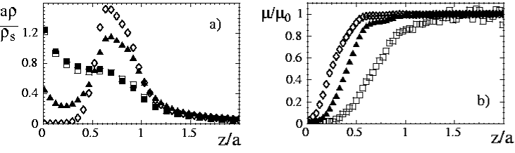
Figure 14: a) Counterion density profiles for Coulomb parameter $\zeta=2.5$ and surface ion density $\rho_{s}a^{2}=0.5$ for different electric field strengths $\tilde{E}=qaeE/k_{B}T=0$ (filled squares), $\tilde{E}=1$ (open squares), $\tilde{E}=10$ (filled triangles), $\tilde{E}=40$ (open diamonds) for a square lattice of fixed surface ions. b) Shown are the rescaled counterion mobility profiles for three different electric field strengths, where $\mu_{0}$ is the bulk ion mobility; same symbols are used as in a).

The main advantage of the Brownian-dynamics technique is that dynamic quantities can be calculated in the presence of externally applied fields even far from equilibrium. As an illustration, we shown in Fig. 14a counterion density profiles for various values of a tangentially applied electric field $\tilde{E}=qaeE/k_{B}T$. The field acts on the mobile counterions and sets them in motion. This is the fundamental setup of electroosmotic and electrophoretic experiments for large colloidal particles. Fig. 14a shows that the density profiles shift to larger distances in the $z$-direction for increasing field strength. By doing this, the counterions avoid being trapped within the surface ion layer, and the conduction is maximized (though hydrodynamic interactions play a role at such elevated field strengths, as has been confirmed recently[70]). In Fig. 14b the corresponding counterion mobility profile is shown. For the smallest field considered, $\tilde{E}=1$ (open diamonds), which belongs to the linear quasi-static regime, the mobility is highly reduced for distances below roughly $z/a=1$, which is plausible since in this distance range surface ions and counterions experience strong excluded-volume interactions and thus friction. The maximal mobility of $\mu/\mu_{0}=1$ is reached quickly for larger separations from the surface. For larger fields the crossover in the mobility profiles moves closer to the surface, and since the density at the wall decreases, the total fraction of immobile counterions goes drastically down. Since the decrease of the mean electrophoretic mobility is caused by a fairly localized layer of immobilized counterions, the integrated relative mobility can be interpreted as the fraction of mobile ions, or, in other words, the fraction of counterions that are not located within the stagnant Stern layer. This gives a dynamical definition of the Stern layer which is unambiguous and connects to the experimentally relevant Zeta potential[123]. The effects seen at elevated field strengths are not relevant experimentally for mono-valent ions, since they correspond to unrealistically high electric field strengths where in fact water is fully oriented; for highly charged objects, however, similar non-equilibrium effects in electric fields do occur. A drastic example of a far-from-equilibrium phase transition is the structural bifurcation that is observed in a two-dimensional electrolyte solution at large electric fields[134]. Here the ions spontaneously form interpenetrating ’traffic lanes’ at large field strengths, which tend to maximize the possible current that is supported by the system. Whether such flux-maximizing states are always realized when one moves far away from equilibrium is presently not clear.

The main message of this example is that the counterion mobility with respect to a tangential field is highly reduced by the presence of surface corrugation[123], which is plausible since counterions are dynamically trapped within the surface-charge layer. The resultant modified boundary condition is relevant for a whole collection of experimental results on the electrophoretic mobility of charged colloids. Simulations that include hydrodynamic interaction essentially confirm the present results and allow to directly connect to experimentally measurable quantities[70]

5 Polyelectrolytes at charged planes: overcharging and charge reversal

For many applications, it is important to adsorb highly charged polymers in a controlled way on planar substrates, for example for the production of DNA chips[135] or the fabrication of charge-oscillating multilayers[136, 137, 138]. Various experiments have been performed with DNA[139, 140] and synthetic polymers with comparable charge density[141, 142]. Important issues are the structure of the adsorbed layer or the amount of adsorbed material at a given set of parameter values (such as salt concentration of the ambient solution, polymer concentration, etc.). Fig. 15a shows atomic-force-microscope pictures of an adsorbed DNA layer on a positively charged substrate, obtained at relatively high salt concentration of $1M$[139]. The analysis of the AFM pictures shows that the adsorbed layer is extremely thin, which is in contrast to the rather diffuse layers that are obtained with neutral polymers. The individual DNA strands have a rather well-defined mutual distance of $B\approx 6nm$ at a salt concentration $c_{s}=1M$, which is larger than the DNA diameter of $D\approx 2nm$. At length scales above $100nm$ the DNA strands change their orientation, the structure resembles a finger print. The lateral distance between DNA strands grows with increasing salt concentration, see Fig.15b[139]. All these findings can be theoretically explained by considering the competition between electrostratic attraction to the substrate and electrostatic and entropic repulsion between neighboring DNA strands[48], as will be shown in the following.

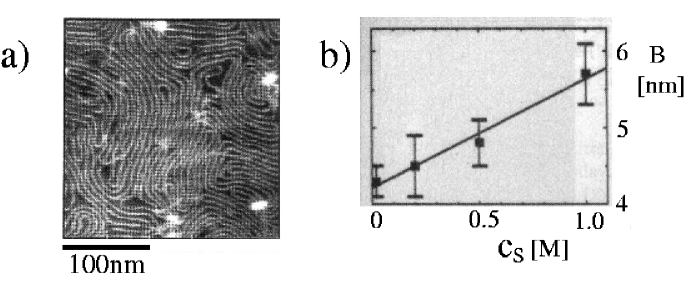
Figure 15: a) AFM picture of a DNA layer adsorbed at an oppositely charged substrate at a salt concentration $c_{s}=1M$. The average lateral distance between DNA strands is $B\simeq 6nm$. b) Mean lateral distance between DNA molecules, $B$, as a function of the salt concentration (reproduced after [139]).

A polyelectrolyte (PE) characterized by a linear charge density $\tau$, is subject to an electrostatic potential created by $\sigma_{s}$, the homogeneous surface charge density (per unit area) on the substrate. Because this potential is attractive for an oppositely charged substrate (which is the situation that was considered in all above-mentioned experiments), it is the driving force for the adsorption and we neglect complications due to additional interactions between surface and PE which have been considered recently[143, 144]. One example for additional effects are interactions due to the dielectric discontinuity at the substrate surface and to the impenetrability of the substrate for salt ions[73]. Within the linearized Debye-Hückel (DH) theory, the electrostatic attractive force acting on a PE section at a distance $\delta$ from the homogeneously charged plane is in units of $k_{B}T$ and per PE unit length

$$f_{\rm att}(\delta)=-4\pi\ell_{B}\sigma_{s}\tau{\rm e}^{-\kappa\delta}.$$ (40)

The screening length $\kappa^{-1}$ depends on the salt concentration $c_{s}$ and ion valency $q$ and is defined via $\kappa^{2}=8\pi q^{2}\ell_{B}c_{s}$. Assuming that the polymer is adsorbed over a layer of width $\delta$ smaller than the screening length $\kappa^{-1}$, the electrostatic attraction force per PE unit length becomes constant and can be written as

$$f_{\rm att}\simeq-4\pi\ell_{B}\sigma_{s}\tau~{}.$$ (41)

For simplicity, we neglect non-linear effects due to counter-ion condensation on the PE (as obtained by the Manning counterion-condensation argument[145]) and on the surface (as obtained within the Gouy-Chapman theory). Although these effects are important for highly charged systems[146], most of the important features of single PE adsorption already appear on the linearized Debye-Hückel level.

Because of the confinement in the adsorbed layer, the polymer feels an entropic repulsion. If the layer thickness $\delta$ is much smaller than the effective persistence length of the polymer, $\ell_{\rm eff}$, as depicted in the side view of Fig. 16a, a new length scale, the so-called deflection length $\lambda$, enters the description of the polymer statistics. We call the persistence length an effective one, because it in principle contains effects due to the electrostatic repulsion between monomers. The deflection length $\lambda$ measures the average distance between two contact points of the polymer chain with the substrate. As shown by Odijk, the deflection length scales as $\lambda\sim\delta^{2/3}\ell_{\rm eff}^{1/3}$ and is larger than the layer thickness $\delta$ but smaller than the persistence length $\ell_{\rm eff}$ [147]. The entropic repulsion follows in a simple manner from the deflection length by assuming that the polymer loses roughly an entropy of one $k_{B}T$ per deflection length.

On the other hand, if $\delta>\ell_{\rm eff}$, the polymer forms a random coil with many loops within the adsorbed layer. The chain can be viewed as an assembly of decorrelated blobs, each containing a subchain of length $L\sim\delta^{2}/\ell_{\rm eff}$, within which the polymer obeys Gaussian statistics. The decorrelation into blobs has an entropic cost of roughly one $k_{B}T$ per blob. The entropic repulsion force per polymer unit length is thus  [147]

$$f_{\rm rep}\sim\left\{\begin{array}[]{llll}&\delta^{-5/3}\ell_{\rm eff}^{-1/3}&{\rm for}&\delta\ll\ell_{\rm eff}\\ &\ell_{\rm eff}\delta^{-3}&{\rm for}&\delta\gg\ell_{\rm eff}~{},\\ \end{array}\right.$$ (42)

where we neglected a logarithmic correction factor which is not important for our scaling arguments.

The equilibrium layer thickness follows from equating the attractive and repulsive forces, Eqs. (41) and (42). For rather stiff polymers and small layer thickness, $\delta<\kappa^{-1}<\ell_{\rm eff}$, we obtain

$$\delta\sim\left(\ell_{B}\sigma_{s}\tau\ell_{\rm eff}^{1/3}\right)^{-3/5}~{}.$$ (43)

For a layer thickness corresponding to the screening length, $\delta\approx\kappa^{-1}$, scaling arguments predict a rather abrupt desorption transition [48]. Setting $\delta\sim\kappa^{-1}$ in Eq. (43), we obtain an expression for the adsorption threshold (valid for $\kappa\ell_{\rm eff}>1$)

$$\sigma^{*}_{s}\sim\frac{\kappa^{5/3}}{\tau\ell_{B}\ell_{\rm eff}^{1/3}}~{}.$$ (44)

For $\sigma_{s}>\sigma_{s}^{*}$ the polymer is adsorbed and localized over a layer with a width smaller than or comparable to the screening length (and with the condition $\ell_{\rm eff}>\kappa^{-1}$ also satisfying $\delta<\ell_{\rm eff}$, indicative of a flat layer). As $\sigma_{s}$ is decreased, the polymer abruptly desorbs at the threshold $\sigma_{s}\simeq\sigma_{s}^{*}$.

From Eq. (43) we see that the layer thickness $\delta$ is of the same order as $\ell_{\rm eff}$ for $\ell_{B}\sigma_{s}\tau\ell_{\rm eff}^{2}\sim 1$, at which point the condition $\delta\ll\ell_{\rm eff}$ used in deriving Eq. (43) breaks down. Let us now consider the opposite limit of a rather flexible chain, $\ell_{\rm eff}<\kappa^{-1}$. If the layer thickness is larger than the persistence length but smaller than the screening length, $\ell_{\rm eff}<\delta<\kappa^{-1}$, the prediction for $\delta$ obtained from balancing Eqs. (41) and (42) becomes

$$\delta\sim\left(\frac{\ell_{\rm eff}}{\ell_{B}\sigma_{s}\tau}\right)^{1/3}~{}.$$ (45)

From the expression Eq.(45) we see that $\delta$ has the same size as the screening length $\kappa^{-1}$ for

$$\sigma_{s}^{*}\sim\frac{\ell_{\rm eff}\kappa^{3}}{\tau\ell_{B}}~{}.$$ (46)

This in fact denotes the location of a continuous adsorption transition at which the layer grows to infinity [48]. The scaling results for the adsorption behavior of a flexible polymer, Eqs. (45)-(46), are in agreement with previous results [148].

Now we generalize the discussion of the single PE chain adsorption and consider the effect of interactions between different adsorbed polymers on a simple scaling level. In order to do so, we assume that the adsorption energy is strong enough such that the polymers essentially lie flat on the substrate, which is the relevant case for describing the experiments shown in Fig.15a. Chain crossings are disfavored, and lateral chain correlations are large enough to induce the polymers to form some type of locally ordered lattice. The formation of this two-dimensionally correlated adsorbed layer is accompanied by a loss of energy and entropy, which will turn out to be important to understand the density of adsorbed chains on the substrate. We follow here the original ideas of Ref. [48], which were in parallel developed by Nguyen et al.[149, 150]. To understand the idea, consider the top view in Fig. 16a, where a lamellar phase is shown where different polymer strands are parallel locally, characterized by an average lamellar spacing $B$. The lamellar phase is stabilized either by steric or by electrostatic repulsions between neighboring polymers; we will in fact encounter both stabilization mechanisms for different values of the parameters. We calculate the free energy and other characteristics of the adsorbed lamellar phase, assuming that we are inside the adsorbed regime of a single polymer. We will also assume, later on, that the desorption transition obtained for the single-chain case also applies to the case of many-chain adsorption. As was shown in Ref. [48], to obtain the complete phase diagram it is sufficient to consider the lamellar phase depicted in Fig. 16a, since other possible phase morphologies are metastable or degenerate. We assume that the distance between neighboring polymer strands, $B$, is much smaller than the effective persistence length, $B<\ell_{\rm eff}$ (which can be checked self-consistently). Since the possible conformations of the adsorbed polymers are severely restricted in the lateral directions, we have to include, in addition to the electrostatic interactions, a repulsive free energy contribution coming from steric interactions between stiff polymers [147]. This is the same type of entropic repulsion that was used before to estimate the pressure inducing desorption from a substrate, Eq.(42), but now including the previously neglected logarithmic cofactor. The total free energy density per unit area and per $k_{B}T$ in the lamellar phase is given by

$$F_{\rm lam}\simeq-\frac{2\pi\ell_{B}\sigma_{s}\tau}{B\kappa}+\frac{1}{\ell_{\rm eff}^{1/3}B^{5/3}}\ln\left(\frac{\ell_{\rm eff}}{B}\right)+F_{\rm rep}~{},$$ (47)

where the first term comes from the electrostatic attraction to the oppositely charged surface (which in accord with the potential used for the repulsion between polymers later on, is taken to be penetrable to ions), the second term is the Odijk entropic repulsion between polyelectrolyte chains [147] and $F_{\rm rep}$ is the electrostatic repulsion within the lamellar array.

To obtain the electrostatic repulsive energy, we first note that the reduced potential created by a charged line with line charge density $\tau$ is at a distance $B$ within the Debye-Hückel approximation given by

$$V_{\rm line}(B)=\tau\int_{-\infty}^{\infty}{\rm d}s\;v_{\rm DH}(\sqrt{B^{2}+s^{2}})=2\ell_{B}\tau K_{0}[\kappa B]~{},$$ (48)

with the Debye-Hückel potential $v_{\rm DH}(r)=\ell_{B}{\rm e}^{-\kappa r}/r$ and where $K_{0}$ denotes the modified Bessel function. The repulsive electrostatic free energy density of an array of parallel lines with a nearest-neighbor distance of $B$ and line charge density $\tau$ can thus be written as

$$F_{\rm rep}=\frac{2\ell_{B}\tau^{2}}{B}\sum_{j=1}^{\infty}K_{0}[jB\kappa]~{}.$$ (49)

This expression is also accurate for rods of finite radius $D$ as long as $D\ll B$ holds. In the limit $B\kappa\ll 1$, when the distance between strands is much smaller than the screening length, the sum can be transformed into an integral and we obtain

$$F_{\rm rep}\simeq\frac{2\ell_{B}\tau^{2}}{B}\int_{0}^{\infty}{\rm d}s\;K_{0}[sB\kappa]=\frac{\pi\ell_{B}\tau^{2}}{B^{2}\kappa}~{}.$$ (50)

This expression neglects effects due to the presence of a solid substrate. For example, and as discussed in Ref. [73], for a low-dielectric substrate the electrostatic interactions are enhanced by a factor of two close to the substrate surface, a rather small effect which will be neglected in the following. Corrections to the approximation in Eq.(50) have been treated in [149, 150]. Since the average adsorbed surface charge density is given by $\sigma_{\rm ads}=\tau/B$, it follows that the self energy Eq. (50) in the limit $B\kappa\ll 1$ is given by $F_{\rm rep}\simeq\pi\ell_{B}\sigma_{\rm ads}^{2}\kappa^{-1}$ and thus is identical to the self energy of a totally smeared-out charge distribution [48]. In this case, lateral correlations therefore do not matter.

In the opposite limit, $B\kappa\gg 1$, when the polymers are much farther apart than the screening length, the sum in Eq. (49) is dominated by the first term and (using the asymptotic expansion of the Bessel function) the free energy density (in units of $k_{B}T$) becomes

$$F_{\rm rep}\simeq\frac{\sqrt{2\pi}\ell_{B}\tau^{2}{\rm e}^{-B\kappa}}{B^{3/2}\kappa^{1/2}}~{}.$$ (51)

In this limit, it is important to note that the smeared-out repulsive energy Eq. (50) is much larger and thus considerably overestimates the actual electrostatic repulsion between polymer strands. Conversely, this reduction of the electrostatic repulsion between polymers results in an enormous overcharging of the substrate, as we will see shortly.

In order to determine the equilibrium distance between the polymer strands, we balance the electrostatic attraction term, the first term in Eq.(47), with the appropriate repulsion term. There are three choices to do this. For $D<\kappa^{-1}<B^{*}<B$ (with some crossover length $B^{*}$ to be determined later on), the electrostatic repulsion between the polymers is irrelevant (i.e. the last term in Eq.(47) can be neglected), and the lamellar phase is sterically stabilized in this case. The equilibrium lamellar spacing is given by

$$B\sim\left[\frac{\kappa}{\tau\sigma_{s}\ell_{B}\ell_{\rm eff}^{1/3}}\ln\left(\frac{\tau\sigma_{s}\ell_{B}\ell_{\rm eff}}{\kappa}\right)\right]^{3/2}~{}.$$ (52)

In all what follows, we neglect the logarithmic cofactor.

For $D<\kappa^{-1}<B<B^{*}$, the steric repulsion between the polymers is irrelevant (i.e. the second term in Eq.(47) can be neglected). The free energy is minimized by balancing the electrostatic adsorption term , the first term in Eq.(47), with the electrostatic repulsion term appropriate for the case $B\kappa>1$, Eq. (51), which leads to the electrostatically stabilized lamellar spacing

$$B\sim\kappa^{-1}\ln\left[\frac{\tau\kappa}{\sigma_{s}}\right].$$ (53)

The adsorbed charge density then follows from $\sigma_{\rm ads}\sim\tau/B$ as

$$\sigma_{\rm ads}\sim\sigma_{s}\frac{\tau\kappa\sigma_{s}^{-1}}{\ln(\tau\kappa\sigma_{s}^{-1})}~{}.$$ (54)

Therefore, the electrostatically stabilized lamellar phase shows always strong charge reversal, since the polymer spacing $B$ is larger than the screening length and thus $\tau\kappa\sigma_{s}^{-1}>1$. This can be seen from comparing the two equations (53) and (54). The crossover between the sterically stabilized lamellar phase, described by Eq.(52), and the lamellar phase which is stabilized by electrostatic repulsion, Eq. (53), occurs when the predictions for $B$ become simultaneously equal to the crossover spacing $B^{*}$, leading to a crossover for a surface charge density of (without logarithmic cofactors)

$$\sigma_{s}^{*}\sim\frac{\kappa^{5/3}}{\tau\ell_{\rm eff}^{1/3}\ell_{B}}~{}.$$ (55)

For $\sigma_{s}$ larger than the crossover value in Eq.(55) the distance between neighboring polymer strands is smaller than $B^{*}$ and the electrostatic stabilization mechanism is at work, for $\sigma_{s}$ smaller than the crossover value in Eq.(55) the lamellar spacing $B$ is larger than the characteristic crossover length $B^{*}$ and the Odijk entropic repulsion dominates. We obtain the interesting result that in the sterically stabilized adsorbed phase the strand separation increases with increasing salt concentration, see Eq.(52), while in the electrostatically stabilized phase the strand separation decreases with increasing salt, see Eq. (53). The intuitive reason for this is clear: in the sterically stabilized phase adding salt diminishes the electrostatic attraction to the substrate, while in the electrostatically stabilized phase the predominant effect of salt is to weaken the repulsion between neighboring PE strands.

The electrostatically stabilized lamellar phase crosses over to the charge-compensated phase when $B$ as given by Eq. (53) becomes of the order of the screening length $\kappa^{-1}$. In the charge-compensated phase, the lamellar spacing is obtained by balancing the electrostatic adsorption energy with the repulsion in the smeared-out limit Eq.(50) and is given by

$$B\simeq\frac{\tau}{\sigma_{s}}~{}.$$ (56)

In this case the adsorbed surface charge density $\sigma_{\rm ads}=\tau/B$ exactly neutralizes the substrate charge density,

$$\sigma_{\rm ads}\sim\sigma_{s}~{}.$$ (57)

The crossover between the charged-reversed phase and charge-compensated phase is obtained by matching Eqs. (53) and (56), leading to a threshold surface charge density of

$$\sigma_{s}^{*}\sim\tau\kappa~{}.$$ (58)

Finally, taking into account that the polymers have some width $D$, there is an upper limit for the amount of polymer that can be adsorbed in a single layer. Clearly, the lateral distance between polymers in the full phase is given by

$$B\simeq D$$ (59)

and thus the adsorbed surface charge density in the full phase reads

$$\sigma_{\rm ads}=\frac{\tau}{D}.$$ (60)

The crossover between the full phase and the compensated phase is obtained by comparing Eqs. (56) and (59), leading to

$$\sigma_{s}^{*}\sim\tau/D.$$ (61)

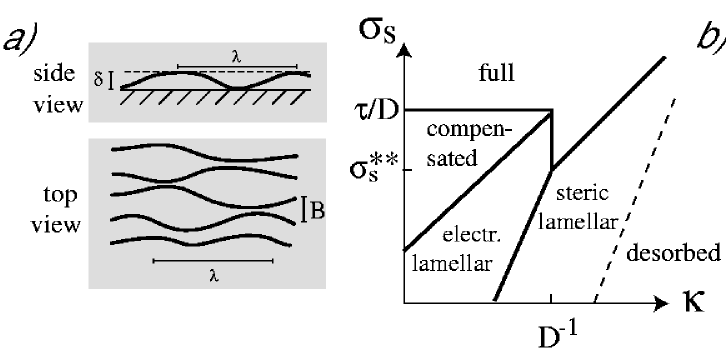
Figure 16: a) Schematic structure of the adsorbed DNA layer in a side view and in a top view, exhibiting the deflection length $\lambda$, the adsorbed layer height $\delta$, and the lateral distance between adsorbed DNA strands, $B$. b) Scaling diagram of the adsorption behavior of a highly charged polymer using logarithmic axes as a function of the surface charge density $\sigma_{s}$ and inverse screening length $\kappa=\sqrt{8\pi\ell_{B}c_{s}}$. The electrostatically stabilized lamellar phase is strongly charge-reversed.

In Fig. 16b we show the adsorption diagram for strongly charged polymers (defined by $\tau\sqrt{\ell_{B}\ell_{eff}}>1$) as a function of the substrate charge density $\sigma_{s}$ and the inverse screening length $\kappa$. The electrostatically stabilized lamellar phase shows strong charge reversal as described by Eq. (54). At slightly larger surface charge densities we predict a charge-compensated phase which is not full (i.e. $B<D$) for a range of surface charge densities as determined by Eqs. (58) and (61). At even larger substrate charge density, the adsorbed polymer phase becomes close packed, i.e. $B\approx D$. We note that since the full phase is not charge reversed, the full phase can consist of a second adsorbed layer (or even more layers, as discussed in [48, 151]). It should however be clear that close to charge compensation the effective substrate charge density an additional layer feels is so small that the condition for adsorption is not necessarily met. At low substrate charge densities the distance between adsorbed polymer strands becomes so large that the entropic repulsion between polymers dominates the electrostatic repulsion, and finally, at even lower charge densities, the polymers desorb. One notes that the transition between the electrostatically and sterically stabilized adsorbed phases, Eq.(55), has the same scaling form (disregarding logarithmic factors) as the desorption transition of semi-flexible polymers, Eq.(44). We have shifted the desorption transition to the right, though, because typically there are attractive non-electrostatic interactions as well, which tend to stabilize adsorbed phases. This is also motivated by the fact that the sterically stabilized phase has been seen in experiments on DNA adsorption, as will be discussed below. The critical charge density $\sigma_{s}$ where the full phase, the electrostatically and the sterically stabilized phases meet at one point, is given by $\sigma^{**}_{s}\sim 1/(D^{5/3}\ell_{\rm eff}^{1/3}\tau\ell_{B})$. In the phase diagram we have assumed that the charge density threshold for the full phase Eq.(61), $\sigma_{s}^{*}\sim\tau/D$, satisfies the inequality $\tau/D>\sigma_{s}^{**}$, which for a fully charged PE at the Manning threshold, $\tau=1/\ell_{B}$, amounts to the condition $\ell_{\rm eff}>\ell_{B}^{3}/D^{2}$, which is true for a large class of PE’s (especially stiff biopolymers such as DNA). As one increases at fixed substrate charge density $\sigma_{s}$ the salt concentration, one moves through the compensated, electrostatically and the sterically stabilized adsorbed phases, before one finally induces desorption. The polymer separation is predicted to first stay constant, then decrease and finally increase, before desorption takes place.

One important result of our discussion is that in the electrostatically stabilized phase the substrate charge is strongly reversed by the adsorbed polymer layer. This can give rise to a charge-oscillating multilayer formation if the adsorption of oppositely charged polymer is done in a second step[136, 137, 138]. The general trend that emerges is that charge reversal is more likely to occur for intermediate salt concentrations and rather low substrate charge density. For too high salt concentration and too low substrate charge density, on the other hand, the polymer does not adsorb at all. In essence, the salt concentration and the substrate charge density have to be tuned to intermediate values in order to create charge multilayers.

In experiments on DNA adsorbed on oppositely charged substrates one typically observes a lamellar phase [139, 140]. In one experiment, the spacing between DNA strands was found to increase with increasing salt concentration [139]. One theoretical explanation invokes an effective interaction between neighboring DNA strands mediated by elastic deformations of the membrane, which forms the substrate in these experiments [152]. In the sterically stabilized regime, the distance between adsorbed polymers increases as $B\sim\kappa^{3/2}$ with the salt concentration, see Eq.(52), which offers an alternative explanation for the experimental findings. It would be interesting to redo DNA adsorption experiments on rigid substrates, where the elastic coupling to the membrane is absent. For high enough substrate charge densities and by varying the salt concentration one should be able to see the crossover from the electrostatically stabilized phase, Eq.(53), where the DNA spacing decreases with added salt, to the sterically stabilized phase, Eq.(52), where the DNA spacing increases with added salt.

5.1 Overcharging by spherical polyions

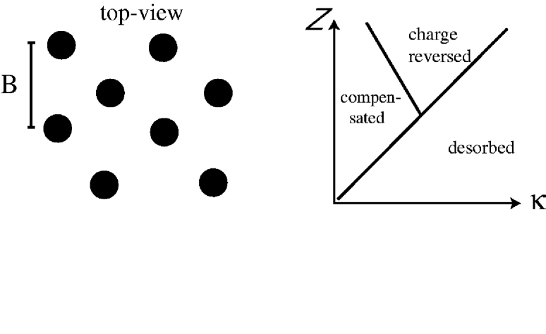
Figure 17: Schematic structure of a layer of adsorbed polyions is shown to the left, characterized by the lateral distance $B$ between adsorbed ions. The right shows the resulting scaling diagram using logarithmic axes as a function of polyion charge $Z$ and inverse screening length $\kappa$, featuring the desorbed phase, a charge reversed phase where more ions adsorb than needed to neutralize the surface charge, and a compensated phase where the adsorbed ions exactly neutralize the surface.

The arguments from the last section for the overcharging of a charged plane by charged polymers can be straightforwardly adapted to the adsorption of spherical polyions on surfaces[150, 153, 154]. Using the DH approximation, the adsorption energy of a polyion of charge $Z$ on a surface of charge density $\sigma_{s}$ in units of $k_{B}T$ is $W_{att}\simeq-4\pi Z\ell_{B}\sigma_{s}/\kappa$ where we assume that the particle radius is smaller than the screening length so that the full particle charge contributes to the attraction. Neglecting logarithmic factors depending on the bulk particle concentration, the desorption threshold is reached when the adsorption energy equals thermal energy, i.e. $W_{att}\simeq 1$. The condition for adsorption is therefore $Z>\kappa/(\ell_{B}\sigma_{s})$. Assuming the particles to form a correlated liquid arrangement on the surface (as depicted in Fig. 17) with a distance between particles larger than the screening length, the repulsion between two nearest neighbors is $W_{rep}\simeq Z^{2}\ell_{B}e^{-B\kappa}/B$. The equilibrium distance of particles is obtained by minimizing the free energy per area,

$$F=(W_{att}+W_{rep})/B^{2}=\frac{Z^{2}\ell_{B}e^{-B\kappa}}{B^{3}}-\frac{Z\ell_{B}\sigma_{s}}{\kappa B^{2}}$$ (62)

which assumes that particles are obtained from some reservoir at vanishing chemical potential. The resulting equilibrium separation is obtained as

$$B\sim\kappa^{-1}\ln(Z\kappa^{2}/\sigma_{s})$$ (63)

and the adsorbed charge density as

$$\sigma_{ads}\simeq\frac{Z}{B^{2}}\sim\sigma_{s}\frac{Z\kappa^{2}/\sigma_{s}}{\ln^{2}(Z\kappa^{2}/\sigma_{s})}.$$ (64)

It can be easily seen that for $Z\kappa^{2}/\sigma_{s}>1$ the surface is overcharged and the distance between adsorbed particles is larger than the screening length (in agreement with our assumption). Thus the condition for overcharging is $Z>\sigma_{s}\kappa^{-2}$. Conversely, for $Z<\sigma_{s}\kappa^{-2}$, the separation between particles becomes smaller than the screening length. A calculation similar to the one in the preceding section shows that the separation in this case is $B\sim\sqrt{Z/\sigma_{s}}$ and the surface is exactly neutralized by the adsorbed layer. The three regimes are shown schematically in Fig. 17 which demonstrates that overcharging is obtained with multivalent ions only above a certain threshold and only at intermediate salt concentrations. Overcharging of charged particles by multivalent counterions is important for a multitude of applications and can change the sign of the electrophoretic mobility[153, 154] and induce macrophase separation [99, 100]. Note that the present argument is analogous to the derivation in [150]. Effects such as non-linear electrostatics (including counterion release) have been included in the literature[6].

6 Polyelectrolytes at charged spheres

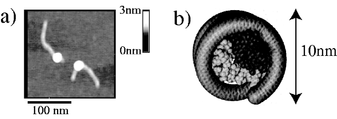
Figure 18: a) AFM pictures of two complexes consisting of a positively charged histone protein and a partially wrapped DNA strand of length 130 $nm$. Adapted after [155]. b) View of the three-dimensional structure of the histone protein; the approximate path of the DNA consists of two full turns (approximately 146 base pairs) and is indicated by a tube (adapted after [156]).

Although DNA is a quite stiff biopolymer and thus resists bending, and although it is highly negatively charged and thus prefers coiled and open structures, the 2m of human DNA is packaged into the cell nucleus which only has a diameter of a few micrometers. To make things even worse, the DNA is not just sitting in the nucleus, but it is all of the time being read, repaired and reshuffled. The mechanism for the folding is ingenious: The DNA is wrapped around a large number of small, highly positively charged almost spherical proteins (called histones), it is thereby partially neutralized and greatly compactified. Fig.18a shows an atomic-force-microscopy picture of two reconstituted complexes consisting of histone proteins and DNA strands of length 130 $nm$[155]. The structures were obtained at a salt concentration of $c_{s}=50mM$. The precise path of the DNA on the proteins can not be resolved, but from the length of the unwrapped DNA portion it can be deduced that roughly one whole turn of DNA is wrapped around the proteins. Fig.18b shows the structure of the complex as obtained from X-ray diffraction on crystallized DNA-histone complexes. Indeed, in the crystalline state (which is not necessarily exactly equal to the solubilized state at room temperatures) the DNA is wrapped twice around the proteins. A huge body of experimental evidence[24, 157]-[170] suggests that the complex is only stable for intermediate salt concentrations between $20mM$ and $500mM$ (the so-called physiological salt concentration in the body is roughly $150mM$ which corresponds to the salt concentration in the sea). For salt concentrations outside this finite range the complex falls apart. As was explained in detail in Section 3.3, salt modulates the electrostatic interactions; it follows that an electrostatic mechanism is the cause for this interesting behavior.

Designing a simple model that can explain the salt and charge dependent behavior of the nucleosomal core particle requires a number of approximations concerning the structure of the DNA, the histone octamer and their interactions. Our strategy was to formulate the simplest possible model which captures the characteristic features responsible for the salt-dependent nucleosomal core structures[171, 172, 173, 174, 175]. In the following we report calculations of the ground state of a single semiflexible polyelectrolyte of finite length which is in contact with a single oppositely charged sphere in the presence of salt. Extensive literature exists on similar model calculations for stiff chains[176, 177], flexible chains[178, 179, 180, 181], for multiple spheres compexing with one polymer[182, 183, 184], for interacting complexes[185, 186, 187, 188] and on simulation studies for complex formation[189, 190, 191, 192, 193]. Polymer form fluctuations away from the ground state will be considered at the end of this section, where it will be shown that the ground state approximation for rather stiff or highly charged polymers is justified. We specifically consider parameters appropriate for the DNA-histone system, approximating the histone as a uniformly charged, impenetrable and solid sphere and the DNA as a uniformly charged semiflexible polymer of length $L$[18, 194]. We deal with the so-called nucleosomal core particles consisting of DNA with 146 base pairs (bp) of length $0.34\,nm$ each, leading to a total DNA length of $L=49.6nm$. The stiffness of the DNA contains charge independent and charge dependent contributions. The former are due to the energy associated with the deformation of hydrogen bonds which stabilize the double helical geometry of DNA and are incorporated by using a semiflexible polymer model with a mechanical bending stiffness. The latter stem from the fact that the negatively charged monomers of the DNA tend to maximize their mutual distance and thus prefer an extended configuration. This electrostatic contribution decreases with increasing salt concentration of the solution and vanishes at the hypothetical limit of infinite salt concentration[195, 196]. The salt independent mechanical persistence length of DNA is therefore the infinite salt limit of the total persistence length, which has experimentally been determined as $\ell_{0}\approx 30\,nm$ [197, 198, 199]. A discussion of different methods to determine the persistence length of DNA is found in [194]. The electrostatic contribution to the persistence length we take into account by explicitly including the electrostatic self energy of DNA conformations, we therefore accurately include the scale-dependence of the electrostatic contribution to the persistence length[21] which is particularly important in our case since the scale of bending (the histone diameter) becomes of the order or even smaller than the screening length.

The histone octamer is approximated as a rigid sphere of radius $R_{\rm hist}=4\,nm$. This is of course only a very rough approximation of the real structure, which is not a perfect sphere and also possesses a corrugated surface with specific binding sites for the DNA. Also, any conformational changes of the histone octamer, which do occur for extremely low or high salt concentration, are neglected. The DNA is modeled as a polymer with radius of $1nm$. In the actual calculation we fix the minimal distance between the sphere center and the DNA monomer centers to be $R=5nm$, which is the sum of histone and DNA radii. The electrostatic interactions between charges on the DNA with each other and the sphere are described by Debye-Hückel (DH) potentials that neglect non-linear effects (such as counterion condensation or counterion release, for which one would need to use the full non-linear Poisson-Boltzmann theory[145, 200, 201]). The main reason for this approximation is that the calculation of the optimal DNA configuration within the PB approach is at present numerically not feasible. For large salt concentrations, the DH approximation becomes valid, as has been shown by calculating the electrostatic contribution to the bending rigidity of a charged cylinder[200, 201].

The energy functional for a given DNA configuration of contour length $L$, parameterized by the space curve ${\bf r}(s)$ and in units of $k_{B}T$, reads

$$H = \frac{\ell_{0}}{2}\int_{0}^{L}{\rm d}s\;\ddot{\bf r}^{2}(s)-\frac{\ell_{B}Z\tau}{1+\kappa R}\int_{0}^{L}{\rm d}s\;\frac{{\rm e}^{-\kappa(|{\bf r}(s)|-R)}}{{|\bf r}(s)|}$$ (65)

$${}+\ell_{B}\tau^{2}\int_{0}^{L}{\rm d}s\;\int_{s}^{L}{\rm d}s^{\prime}\;\frac{{\rm e}^{-\kappa|{\bf r}(s)-{\bf r}(s^{\prime})|}}{{|\bf r}(s)-{\bf r}(s^{\prime})|}$$

where we implicitly assume that the DNA molecule is inextensible, i.e., $|\dot{\bf r}(s)|=1$. The first term describes the mechanical bending energy, proportional to the bare persistence length $\ell_{0}$, where the curvature $\ddot{\bf r}(s)$ is given by the second derivative of ${\bf r}(s)$ with respect to the internal coordinate s. The second term describes the electrostatic attraction between the sphere and the DNA[10]. The charge of the sphere in units of the elementary charge e is denoted by $Z$ and the linear charge density of the DNA (in units of e) is denoted by $\tau$. A key ingredient of the Debye-Hückel-theory is the screening of electrostatic interactions, which is quantified by the Debye-Hückel screening length $\kappa^{-1}$. It measures the distance beyond which the interaction between two charges is exponentially damped. For monovalent salt one finds $\kappa^{2}=8\pi\ell_{B}c_{s}$, where $c_{s}$ is the salt concentration. At 0.1 molar concentration in water, i.e. at physiological conditions, one has $\kappa^{-1}\approx 1\,nm$. The third term describes the electrostatic repulsion between charges on the DNA. We therefore have two terms that tend to straighten the DNA, namely the mechanic bending energy and the electrostatic repulsion between DNA monomers. The former is salt independent, whereas the latter looses importance with increasing salt concentration. These repulsions are balanced by the sphere-DNA electrostatic attraction, which favors bending of the DNA in order to wrap it around the sphere, but also becomes weaker for increasing salt concentration. It transpires that salt will determine the DNA structure in a rather subtle way, as will be demonstrated by our numerical results.

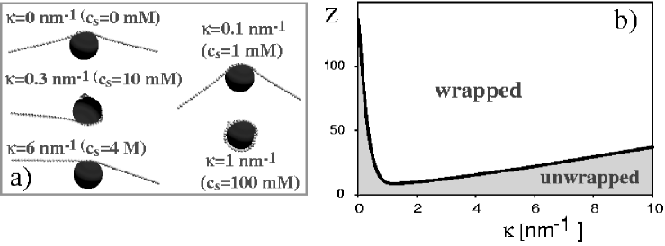
Figure 19: a) DNA configurations as obtained by numerical minimization of the free-energy expression Eq.(65) for fixed sphere charge $Z=25$ and various salt concentrations. As can be seen, the DNA is only wrapped for intermediate values of the salt concentration. b) Global phase digram, featuring the wrapping transition as a function of the inverse screening length (proportional to the square root of the salt concentration, $\kappa\sim c_{s}^{1/2}$), and sphere charge $Z$.

In analyzing the model defined by Eq.(65) we take advantage of the short length of the DNA strand, $L=50\,nm$, compared to the effective persistence length, which is at least of the order of the bare persistence length, $\ell_{0}=30\,nm$. As a starting point, we therefore neglect fluctuations and undulation forces [171] between DNA and sphere and apply a ground state analysis to the model. This consists of finding the configuration of the DNA that minimizes Eq. (65) with the constraints $|\dot{\bf r}(s)|=1$ (no stretching) and $|{\bf r}(s)|\geq R$ (impenetrability of sphere). We also use Debye-Hückel-potentials with the full DNA line charge $\tau=2/0.34\,nm$, corresponding to the maximal degree of dissociation of DNA (and neglecting counterion-condensation effects[145] which have been investigated in [173]).

In Fig. 19 we show a series of DNA configurations obtained for a fixed sphere charge $Z=25$ and for inverse screening lengths ranging from $\kappa=0\,nm^{-1}$ to $6\,nm^{-1}$. In the pure Coulomb case with no added salt, the sphere is located in the middle of the DNA, and the two arms are slightly bent towards the sphere. As the salt concentration is increased from $\kappa=0$ to $\kappa=0.1\,nm^{-1}$, the deflection of the DNA arms increases continuously. Interestingly, the binding of the DNA onto the sphere becomes stronger as one weakens the electrostatic interactions. Upon further increase of salt concentration, the two-fold rotational and the mirror symmetries are broken, see the configuration at $\kappa=0.30\,nm^{-1}$. One of the DNA arms is totally wrapped around the sphere. As $\kappa$ is increased further, the extended arm is more and more pulled onto the sphere until at $\kappa=1\,nm^{-1}$ the DNA is fully adsorbed onto the sphere and the two-fold rotational symmetry is restored. At $\kappa=6\,nm^{-1}$ a strongly discontinuous transition occurs in which the DNA completely dewraps from the sphere. The dewrapped state at high salt concentration is markedly different from the state at zero salt. There is only one short region of nonzero bending of the DNA connecting two basically straight arms. This sequence of complexation structures demonstrates one of our main results, namely that the wrapped DNA conformation is only stable for intermediate salt concentrations, explaining a large set of experimental results for nucleosomal core particles[24].

We summarize our results for a DNA length of $L=50nm$ in the phase diagram presented in Fig.19b. In the absence of salt, $\kappa=0$, the wrapping transition occurs at $Z=133$ (in agreement with previous theoretical predictions[181]). In agreement with experiments [24], complexation is most pronounced at intermediate salt concentrations. For low salt concentration, the strong DNA-DNA repulsion prevents complexation, for high salt screening weakens the DNA-sphere attraction sufficiently so that the mechanical bending resistance induces dewrapping. The minimal sphere charge to wrap the DNA, $Z\approx 10$, is obtained for $\kappa^{-1}\approx 1\,nm$ ($c_{s}\approx 0.1\,M$ for monovalent salt), corresponding to physiological conditions. Since the total charge on the DNA is about $300$, the complex is strongly overcharged for all $Z<300$, i.e., in the whole wrapped region shown in the phase diagram. The high-salt prediction for the wrapping transition can be obtained analytically by locally balancing the various terms in the energy functional, Eq. (65), namely the bending energy per unit length, $H_{\rm bend}\simeq\ell_{0}/2R^{2}$, and the electrostatic attraction per unit length in the limit $\kappa R>1$, $H_{\rm att}\simeq\ell_{B}Z\tau/\kappa R^{2}$, leading to $Z_{\rm wrap}\simeq\ell_{0}\kappa/2\ell_{B}\tau$, in agreement with the numerical results[171].

These results highlight a peculiarity of electrostatic complexation phenomena, and is mirrored by an at first sight perplexing approximation used in our model calculation: We do use the Debye-Hückel approximation for the interaction between charges on the sphere and on the DNA, which amounts to taking into account positional fluctuations of the salt ions within a Gaussian approximation[68]. However, we do not take into account positional fluctuations of the DNA itself, but concentrate on the ground state instead. The reason for the different treatment of salt ions and DNA monomers is that the total amount of charge per statistically independent unit is $q=1$ for monovalent ions but roughly $q\simeq 180$ for one persistent segment of DNA of length $L\simeq\ell_{0}$. Therefore fluctuations are rather unimportant for the DNA structure (except for very large salt concentrations where a desorption transition does occur which can be treated using similar methods as used for the desorption of polyelectrolytes on planar substrates in the preceding section[171]) but are of extreme importance for the counterion clouds. To make these statements quantitative, we estimate now the conformational entropy which can be obtained by a normal-mode analysis of the chain fluctuations around the ground state configuration.

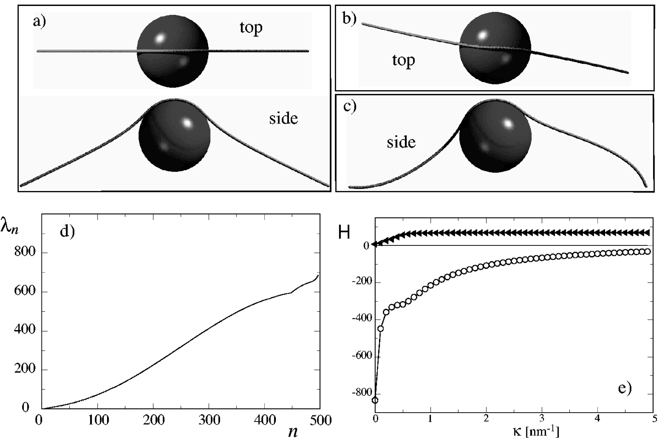
Figure 20: a) Ground-state configuration of the complex for a sphere charge $Z=40$ and zero salt concentration $\kappa=0$. b) Second and c) sixth excited state. The second eigen mode breaks the mirror symmetry but leaves the two-fold rotational symmetry intact, while the sixth eigen mode breaks the two-fold rotational symmetry. d) Eigenvalue spectrum for $Z=20$ and $\kappa=0$. e) Ground state energy (open symbols) and Gaussian fluctuation contribution (filled symbols) for charge $Z=20$ as a function of the inverse screening length $\kappa$. The fluctuation contribution is obtained by integrating out the complete eigenmode spectrum shown in d).

Let us assume that the ground state configuration of the chain is given by the space curve ${\bf r}_{0}(s)$ which minimizes the energy functional $H$ in Eq.(65) according to $\delta H/\delta{\bf r}(s)=0$. In the actual calculation the space is discretized and the actual degrees of freedom are bond angles, but this is not important for the present presentation. For small fluctuations around the ground state, the effective Hamiltonian of the complex may be expanded around the minimum up to second order as

$$H=H[{\bf r}_{0}]+\frac{1}{2}\int dsds^{\prime}[{\bf r}(s)-{\bf r}_{0}(s)]H^{(2)}(s,s^{\prime})[{\bf r}(s^{\prime})-{\bf r}_{0}(s^{\prime})]$$ (66)

where the Hessian matrix associated with the effective Hamiltonian, is defined as

$$H^{(2)}(s,s^{\prime})=\bigg{(}\frac{\delta^{2}H}{\delta{\bf r}(s)\delta{\bf r}(s^{\prime})}\bigg{)}_{{\bf r}={\bf r}_{0}}$$ (67)

It characterizes the spectrum of chain excitations within the harmonic (or Gaussian) approximation. The normal modes of a complex are obtained by diagonalizing the Hessian, using the discrete notation ${H}^{(2)}_{mn}A_{np}=\Lambda_{mn}A_{np}$, which is solved numerically for the matrix of eigen-modes, $A_{np}$, and the diagonal matrix of eigen-values, $\Lambda_{mn}=\lambda_{n}\delta_{mn}$.

In Figure 20, we show in a) the ground state and in b) and c) the second and the sixth excited states of the complex, respectively[203]. The parameter values chosen are $Z=40$ and $\kappa=0$. As seen, the ground state’s mirror symmetry is broken in the second excited state and the two-fold rotational symmetry is broken in the sixth excited state. The latter eigen-mode can be viewed as a translational motion of the bound sphere along the PE chain. In Fig. 20d we show the mode spectrum obtained from the Hessian via diagonalization. We discretize the chain by 250 beads, we therefore have a total of 500 eigenmodes. From the fluctuation spectrum the configurational entropy can be obtained since the configurational integral can be performed on the Gaussian level exactly in tems of the normal modes[203]. In Fig. 20e we show the ground state energy of the complex (open symbols) and the configurational entropy contribution (filled symbols) as a function of $\kappa$. For both contributions the reference state of a free polymer has been subtracted. The entropy is positive, as it costs configurational freedom to bind a polymer onto a sphere, the ground-state energy is negative as sphere and polymer do attract. When the two contribution have equal magnitude (roughly at $\kappa\approx 3nm^{-1}$) the total free energy gain upon complexation is zero. This signals an entropy-driven unbinding transition which of course depends on the solution concentration of DNA strands and histone spheres via the law-of-mass action[203]. It follows that in some regions of the phase diagram shown in Fig.19 the complex is dissolved into its constituting parts, depending on the bulk concentrations.

7 Polyelectrolytes at charged cylinders

When semiflexible charged polymers are mixed with much stiffer oppositely charged polymers, a complex forms where the more flexible polyelectrolyte (PE) wraps around the stiff polymer[204, 205, 206, 150, 207, 208, 209]. Experimentally, such complexes itself fold up into toroidal or stem-like structures under dilute conditions[210, 211]; in more concentrated solutions, bundles and networks are observed[212]. In this section we try to understand the morphology of the underlying molecular complex, namely the conformation of the wrapping polymer: does it form a helix or does it adsorb in (one or more) parallel straight strands onto the cylinder? Using linear (Debye-Hückel) theory, supplemented by nonlinear (counterion release) arguments[205], we find transitions between both morphologies as the salt concentration (or other parameters) are varied.

Most of the current interest in such complexes comes from their potential applications in gene therapy: The main problem here is to introduce genetic material into patients’ cell nuclei, a process called DNA transfection. The classical viral strategies are highly effective in transfecting DNA but may provoke immune reactions of the body, switch back to their lethal origin or lead to a stable transformation of target cells (advantageous in some cases though in general undesirable)[213, 214]. Nonviral transfection strategies avoid these difficulties at the price of much reduced effectiveness[214]. Still, they hold promising potential for further development and refinement. The polyfection scheme consists of complexing DNA with physiologically tolerated polycations, such as polypeptides or synthetic polycations [214, 215] and shows relatively high efficiency, especially with confluent (non-dividing) cells[216]. As a major advantage, the properties of these self-assembling polyplexes can be controlled rather reliably by for example varying the mass or charge density of the polycations[217], by using block-copolymers with a cationic block and an uncharged block which forms some type of protection layer against coagulation or degradation[218], and finally by linking target-specific ligands to the polymer chains[219].

The microscopic structure of polyplexes is not very well understood. Electron micrographs of DNA-polylysine complexes exhibit highly condensed torus or stemlike structures[210], very similar to what is seen with DNA condensed by multivalent counterions[220]. More recent AFM studies demonstrated that condensation involves five to sixfold overcharging of the DNA by peptide charges at elevated salt concentration[211]. The underlying molecular structure of polycation-DNA complexes (toroidal or stemlike), which involve multiply packed DNA loops, is not resolved in these experiments. X-ray diffraction measurements, on the other hand, showed that polylysine wraps helically around the DNA molecule (and at low salt concentrations neutralizes the DNA charges), while polyarginine, a cationic polypeptide with a different backbone flexibility, shows a different wrapping mode[221]. Similar complexation is obtained by mixing DNA with a rather bulky cationic dendrimeric polymer: AFM pictures demonstrate that in this case the DNA wraps around the dendro-polymer[222]. This essay, with potential gene-therapeutical applications, holds the advantage that the physical properties of the complex and the effects of various parameters can be studied in great detail and with comparative ease. From all the above listed experiments, it is clear that the salt concentration of the surrounding medium, the charge of the complexing polycations, and their flexibility can induce different morphologies of the polyplex. The possibility and mechanism of DNA-overcharging by adsorbed polycations is interesting from a fundamental point of view[205, 181, 150, 171], although it has been shown that optimal transfection yield is obtained with neutral complexes[217, 219] (despite the naive expectation that cationic complexes would interact more favorably with the typically negatively charged cell and endosomal walls).

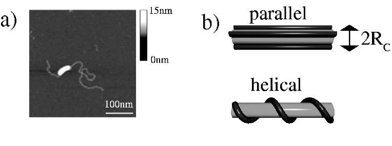
Figure 21: a) AFM pictures of a DNA strand of lengh $L_{P}=850nm$ which is partially wrapped around a $L_{C}=50nm$ long cationic dendropolymer (reproduced from Ref.[222]). b) The two posibble wrapping morphologies that are theoretically studied and compared.

In Fig.21a a DNA-dendropolymer complex is shown which consists of a DNA strand of length $L_{P}\approx 850nm$ wrapped around a cylindrical dendropolymer of length $L_{C}\approx 50nm$ and radius $R_{C}\approx 3nm$. The DNA is complexed as a single strand with the dendropolymer, from the wrapped DNA length (which can be determined by measuring the length of the non-wrapped DNA sections) it follows that the DNA almost fully covers the dendropolymer surface. Since no loops are seen that emerge from the complex, it is suggested that the DNA wraps helically around the core. In fact, more DNA wraps than is needed to neutralize the dendropolymer core, the precise amount of wrapped DNA turns out to be salt dependent[223].

In this section we analyze the complexation between a charged rigid cylinder and an oppositely charged semiflexible polyelectrolyte. The parameters in our model are the linear charge densities of the uniformly charged cylinder and the PE, $\tau_{C}$ and $\tau_{P}$, the cylinder radius $R_{C}$ and the bare PE persistence length $\ell_{0}$. On the linear level the interaction between all charges is given by the bulk Debye-Hückel (DH) potential $v_{DH}(r)=\ell_{B}\exp(-\kappa r)/r$ where $r$ is the distance between charges, $\ell_{B}$ is the Bjerrum length, $\ell_{B}=e^{2}/\!4\pi\varepsilon\varepsilon_{0}\,k_{B}T$, and $\kappa^{-1}$ is the screening length. The DH approximation is valid for weakly charged PEs, elevated salt concentrations and, as is explained in Ref.[206], for complexes close to electroneutrality. Effects due to dielectric boundaries, additional non-electrostatic interactions, inhomogeneous charge distributions on the cylinder and on the PE, polymer confinement (which are all neglected) and counterion release are of only secondary importance for the resulting phase diagrams, since we always compare different morphologies of roughly the same amount of adsorbed PE. It is the free-energy difference between different morphologies that we are most interested in, not their absolute values[206]. The thermodynamic ensemble we consider is the one where PE is present in excess, i.e., we minimize the free energy per cylinder unit length, treating the non-adsorbed PE as a reference state the electrostatic self energy of which therefore has to be subtracted. We also neglect end effects which will only be important if the screening length becomes larger than the cylinder length. This is the ensemble that is indeed relevant to describe the experimental situation in Fig.21a. The thermodynamic ensemble considered in Ref.[208] is different since the cylinder self-energy was not subtracted; it consequently gives results very different from our scheme. We compare two morphologies, namely a helical arrangement of the PE, where a single helix, characterized by the length ratio of the wrapped polymer section and the cylinder length, wraps around the cylinder (see Fig.21b), and the straight morphology, where $n$ parallel strands of PE adsorb on the cylinder. We minimize both configurational energies with respect to the relative amount of wrapped polyelectrolyte (neglecting configurational fluctuations around the ground state which are unimportant for rather stiff and highly charged PEs) and compare the two resulting free energies to determine the stable phase. This comparison, which is done numerically in the general case, shows that both morphologies compete closely with each other.

As can be seen in the phase diagram Fig.22a, which is obtained in the limit when the wrapping polymer is totally flexible and has no bending stiffness, $\ell_{0}=0$, the helical phase is favored at low salt concentrations (to the left) and highly charged wrapping polymers ($\tau_{P}/\tau_{C}\gg 1$), while the parallel morphology is favored at high salt concentrations. As the charge density of the wrapping polymer increases, as one moves up in the phase diagram, the number of adsorbed strands in the parallel phase goes down. Fig.22b shows for the specific charge density ratio $\tau_{P}/\tau_{C}=0.5$ that the amount of wrapped polymer, characterized by the ratio of the contour length of the wrapped polymer and cylinder length, $L_{P}/L_{C}$, grows with increasing salt concentration (the desorption transition, which is expected to occur at high salt concentrations in the absence of additional non-electrostatic attractive forces is not shown but follows the same rules as outlined in Section 5). For line charge ratio $\tau_{P}/\tau_{C}=0.5$ the complex would be neutral for a wrapping ratio $L_{P}/L_{C}=2$. As a matter of fact, more polymer wraps around the core cylinder than is needed to actually neutralize the complex (in agreement with the experimental results[222]). As the salt concentration increases the overcharging is even further enhanced, also in agreement with experiments[223].

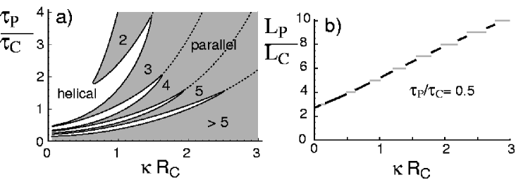
Figure 22: a) Phase diagram of the polyelectrolyte-cylinder complex as a function of the linear-charge density ratio $\tau_{P}/\tau_{C}$ and the inverse rescaled screening length $\kappa R_{C}$ for vanishing persistence length of the wrapping polymer, $\ell_{0}=0$. The helical phase (white) dominates at low salt concentration (small $\kappa R_{C}$) while the straight configuration (shaded; number of adsorbed PE strands is indicated and direct transitions between states with different numbers of adsorbed strands are denoted by broken lines) is realized at large $\kappa R_{C}$. b) Relative amount of wrapped PE, $L_{P}/L_{C}$, for zero persistence length $\ell_{0}=0$ for a line charge density ratio of $\tau_{P}/\tau_{C}=0.5$, corresponding to a horizontal cut through the phase diagram Fig.22a. In the helical phase the wrapping parameter (and thus the overcharging of the cylinder) continuously increases as $\kappa R_{C}$ grows, while the straight configuration is characterized by integer values.

The overcharging in the low-salt limit is easily understood analytically. For simplicity we consider the parallel morphology with $n$ adsorbed polymers with line charge density $\tau_{P}$ at a cylinder of line charge density $\tau_{C}$. In the limit of low salt, $\kappa R_{C}\rightarrow 0$, the electrostatic potential of a charged cylinder, which is derived in Eq.(48) on the Debye-Hückel level, shows a logarithmic behavior. The potential at the cylinder surface is given by $-2\ell_{B}\tau_{C}\ln(\kappa R_{C})$. The total attractive free energy of $n$ adsorbed polyelectrolytes is thus in the low-salt limit per unit length given by

$$F_{\rm att}\simeq 2n\ell_{B}\tau_{C}\tau_{P}\ln(\kappa R_{C}).$$ (68)

Between the $n$ adsorbed polymers there are $n(n-1)/2$ repulsive pair interactions, all of the same logarithmic type. Clearly, the distances between the various pairs are all different, but since the repulsion is logarithmic these differences give negligible additive contributions to the resulting total repulsive free energy, which can be written as

$$F_{\rm rep}\simeq-n(n-1)\ell_{B}\tau_{P}^{2}\ln(\kappa R_{C}).$$ (69)

The number of adsorbed polymers results from minimization of the sum of the repulsive and attractive contribution, $\partial(F_{\rm att}+F_{\rm rep})/\partial n=0$, and is given by

$$n=L_{P}/L_{C}=1/2+\tau_{C}/\tau_{P}.$$ (70)

It equals the ratio of the wrapped polymer length and the cylinder length, $L_{P}/L_{C}$, which is the quantitiy that is plotted in Fig.22b. The number of adsorbed strands $n$ is an integer quantity. However, the analogous calculation for the helical phase in the low-salt limit gives the same result as Eq.(70). Both phases turn out to be degenerate for integer values of the wrapping ratio $L_{P}/L_{C}$. The result Eq.(70) is in agreement with the numerical data displayed in Fig.22b, and predicts for the case $\tau_{P}/\tau_{C}=0.5$ the wrapping length ratio $L_{P}/L_{C}=5/2$ in the zero salt limit $\kappa R_{C}\rightarrow 0$ (note that the asymptotic approach of this limit is logarithmically slow, see [206]). The effective charge of the complex is in the same low-salt limit from Eq.(70) predicted to be

$$\tau_{\rm eff}=n\tau_{P}-\tau_{C}=\tau_{P}/2$$ (71)

and was also obtained using an alternative approach[224]. This result shows that in the low-salt limit the complex will have the same charge sign as the wrapping polymer, the usual wording for this is that the complex is overcharged. The effective charge density of the complex amounts to half the one of the wrapping polymer. Therefore, if the negatively charged DNA wraps around a cationic dendropolymer, the complex will have a net negative charge, if however a flexible cationic polypeptide wraps around the negatively charged DNA, the resulting complex will be positively charged. These qualitative trends are in agreement with experiments, and they show how to tune the charge of a polyelectrolyte complex by changing the ratio of the bending rigidities of the cationic and anionic polymers involved in forming the complex.

8 Polyelectrolytes in electric fields

The behavior of flexible polyelectrolytes (PE) exhibits a number of remarkable features which are due to the electrostatic coupling between polymeric and counterion degrees of freedom. Noteworthy is the sequence of PE conformations which is observed in simulations as the electrostatic coupling between the charges on the PE and the counterions is increased[225, 226, 227, 228]. Experimentally, the coupling can be tuned by changing temperature, dielectric constant of the solvent, counterion valency/size and charge density of the PE. For very small coupling the PE resembles a neutral polymer since the electrostatic repulsion between monomers is very small. As the coupling increases, the monomer-monomer repulsion leads to a more swollen configuration (the standard PE effect). However, as the coupling further increases, counterions condense on the PE, decrease the repulsion between monomers and the PE starts to shrink. Finally, at very large electrostatic coupling, the PE is collapsed to a close-packed, almost charge-neutral condensate which contains most of its counterions. A similar sequence is experimentally seen with synthetic PEs[229] and DNA[230, 231, 232].

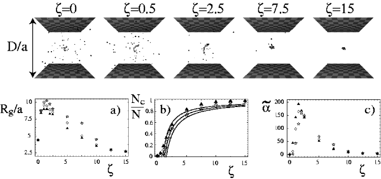
Figure 23: Simulation snapshots of a PE with $N=50$ monomers in a cubic box of diameter $D/a=100$ for various values of the coupling parameter $\zeta$. a) Radius of gyration $R_{g}/a$, b) average rescaled number of condensed counterions $N_{c}/N$, and c) polarizability $\tilde{\alpha}=k_{B}T\alpha/(qea)^{2}$ for a PE of monomer number $N=50$ and box sizes $D/a=200$ (stars), $D/a=100$ (diamonds), $D/a=50$ (filled triangles).

This well-known behavior is visualized in Fig.23 where we show in the top panel a few snapshots of a Brownian dynamics simulation for a PE chain with $N=50$ monomers for different values of the Coulomb parameter

$$\zeta=q^{2}\ell_{B}/a$$ (72)

where $a$ is the diameter of monomers and counterions (which are both modelled as hard spheres) and $q$ is the valence of monomers and counterions (which are the same). The PE behavior is best quantified by the radius of gyration $R_{g}$, defined as

$$\tilde{R}_{g}^{2}=\frac{1}{2N^{2}}\sum_{i,j,=1}^{N}\langle({r}_{i}-{r}_{j})^{2}\rangle=\frac{1}{N}\sum_{i=1}^{N}\langle({r}_{i}-{R}_{com})^{2}\rangle$$ (73)

where the sum includes PE monomers only and ${R}_{com}$ denotes the center of mass in rescaled coordinates defined as

$${R}_{com}=\frac{1}{N}\sum_{i=1}^{N}{r}_{i}.$$ (74)

The rescaled radius of gyration in Fig.23a shows for the various box sizes used a maximum at $\zeta\approx 3/2$. In the simulations, the PE and all counterions are confined in a cubic box of width $D$. There is a systematic trend in the data showing that the radius of gyration is larger for larger box sizes. This can be understood by studying the degree of counterion condensation. The number of condensed counterions (rescaled by the total number of counterions), $N_{c}/N$, is shown in Fig.23b and depends weakly on the box size $D$: The bigger the box the smaller the number of condensed counterions. We rather arbitrarily define a counterion as condensed when its center is closer than $2a$ to any monomer center, i.e. when there is at least one monomer closer than two times the diameter (we checked that our results depend only very weakly on the precise distance chosen to discriminate between condensed and uncondensed counterions). Since the number of condensed counterions goes down with increasing box size, it is fairly easy to understand that the effective PE repulsion goes up and thus the radius of gyration increases. The solid lines in Fig.23b denote the standard Manning prediction for the number of condensed ions[145] corrected by the finite length of the PEs[233].

In Fig.23c the polarizability according to the fluctuation-dissipation theorem,

$$\tilde{\alpha}=\frac{k_{B}T\alpha}{(qea)^{2}}=\frac{\langle P^{2}\rangle}{3(qea)^{2}}$$ (75)

is shown. The dipole moment of the complex is denoted by $P$ and is measured with respect to the PE center of mass. The resultant polarizability shows a strong $\zeta$ dependence and qualitatively follows the trend of the radius of gyration shown in Fig.23a. The classical result for the polarizability of a sphere with radius $R$ and uniformly distributed charge $Q$ around an opposite point charge $Q^{\prime}$ is for $Q=Q^{\prime}$ given by $\alpha=4\pi\epsilon R^{3}$[32] or, in rescaled units with $\tilde{R}=R/a$, $\tilde{\alpha}=\tilde{R}^{3}/\zeta$. Identical results are obtained from the Clausius-Mossotti equation[33] or using different, more complicated charge distributions. In fact, by comparing the radius of gyration and the polarizability, one can show that these simple relations also hold for the collapsed PE chain.

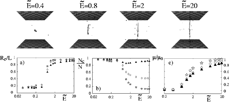
Figure 24: PE snapshots for fixed Coulomb parameter $\zeta=10$ and box size $D/a=100$ and various rescaled field strengths, exhibiting an unfolding transition at $\tilde{E}=qeaE/k_{B}T\approx 0.4$. a) Rescaled end-to-end radius $R_{e}/L$, where $L=aN$, b) number of condensed counterions $N_{c}/N$, and c) relative mobility of PE monomers for box sizes $D/a=200$ (stars), $D/a=100$ (diamonds), $D/a=50$ (filled triangles) for $\zeta=10$.

All these phenomena concern the static, equilibrium behavior of PEs. In electrophoretic experiments, PEs are subject to external electric fields and the resulting mobility is measured[234, 235]. Such techniques are widely used to separate DNA and charged proteins according to their molecular weight. In these situations, the electric field induces motion of ions and PEs, thus dissipation of energy, and one is facing a non-equilibrium problem. In the following, we briefly discuss the effects of electric fields on PE condensates. In contrast to previous theories, where the counterions are not taken into account explicitly or their coupling to the PE is rather weak[236, 237, 238], we start from a strongly coupled (collapsed) PE-counterion system and investigate the resultant effects for large electric fields (i.e. far from equilibrium). We choose a Coulomb coupling of $\zeta=10$. Fig.24 shows a few snapshots for increasing field strength, exhibiting an unfolding transition of the PE condensate at a critical field strength. The non-equilibrium unfolding transition manifests itself as a rather abrupt increase of the rescaled end-to-end radius $R_{e}/L$, which in Fig.24a is shown for $\zeta=10$ and various box sizes as a function of the rescaled applied field $\tilde{E}=qea{E}/k_{B}T$. The contour length of the PE is denoted by $L$. The number of condensed counterions in the high-field extended configuration exhibits a dramatic dependence on the box size, see Fig. 24b. It approximately equals the ratio of polymer length and box size, $N_{c}/N\approx L/D$, since the counterions in the large-electric-field limit are distributed almost evenly along the electric-field direction. In the absence of interactions between PE monomers and counterions, or in the limit of infinite dilution, the electrophoretic mobility $\mu$ (which is equivalent to the conductivity) equals the bare mobility $\mu_{0}$ for all charged particles. In Fig. 24c we show the PE monomer mobility for different box sizes as a function of the external field. For small fields the mobility is almost zero, i.e., the condensed counterions slow down the PE considerably. As the field strength increases, the rescaled mobility $\mu/\mu_{0}$ slowly approaches unity. This is an extreme example of the Wien effect, which was originally observed for simple electrolyte solutions. It transpires that the non-equilibrium effect of strong external driving fields can, together with strong electrostatic interactions, lead to qualitatively new features such as field-driven conformational transitions and complex dissolution. At a critical field strength, a collapsed PE unfolds and orients in the direction of the field. Since the PE mobility is expected to change drastically at the unfolding transition, this transition should be detectable by mobility measurements and in turn could be used for efficient separation of PEs of different length[233].

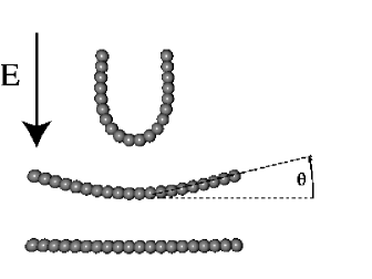
Figure 25: Snapshots for an elastic, semiflexible rod, characterized by a bare persistence length $\ell_{0}$, that is driven down in a quiescent, viscous liquid by a total force $F$ that is acting equally on all monomers. The stationary shapes are obtained for rescaled driving forces of $L^{2}F/(\ell_{0}k_{B}T)$ = 760, 76,7.6, from top to bottom. Hydrodynamic effects lead to a deformation and, consequently, to an orientation of the rod.

So far we neglected hydrodynamic effects, that means that the flow can freely penetrate the polymer and no hydrodynamic interactions occur when objects move past each other. Clearly, one would expect a whole number of interesting kinetic effects to turn up when polymers move in strong fields in viscous fluids. Probably the most basic effect concerns a hydrodynamic mechanism for the orientation of polymers as they move through quiescent liquids. The arguments presented above show that charged polymers align along their long axis along an electric field. What happens when hydrodynamics are taken into account?

For orthotropic bodies, that is for bodies with three mutually orthogonal planes of symmetry such as cylinders, the hydrodynamic coupling term between translational and rotational motion vanishes[239]. This result is valid only in the hydrodynamic limit of small Reynolds numbers (i.e. small bodies and low velocities), which is the relevant regime for almost all viscous solvent effects of nanoscopic materials. It implies that a rigid cylindrical particle, such as a rod-like synthetic or biological polymer, that is driven by a homogenous external force (be it gravitational or electric in the case when the particle is charged) and as a result is moving through a quiescent fluid, is hydrodynamically not oriented in any particular way: the orientational distribution function will be uniform, not favoring parallel or perpendicular orientation with respect to the direction of motion. In contrast, for elastic rods hydrodynamic effects lead to a bending and therefore reduction in symmetry[240, 241, 242]. The hydrodynamic translational-rotational coupling becomes finite and in consequence sedimenting rods orient perpendicularly to the direction of motion. This is graphically illustrated in Fig.25 where we show stationary shapes of a semiflexible polymer that is moving downwards under the action of a force acting uniformly on the monomers. The structures are obtained with a simulation code that takes hydrodynamics into account on the Stokes or creeping-flow level, including the effects of elasticity and thermal fluctuations[242]. The relevant parameters are the mechanical bending rigidity, expressed in terms of the bare persistence length $\ell_{0}$, the total force acting on the rod, $F$, related to an electric field $E$ via $F=qeEN$, and the length $L$. The structures depicted in Fig.25 are obtained for rescaled driving forces of $L^{2}F/(\ell_{0}k_{B}T)$ = 760, 76,7.6, from top to bottom. It is seen that the rod is deformed, but also that it is oriented with respect to the direction of motion. The mechanism is quite simple to understand: The external force drives all monomers in the same way; due to hydrodynamic interactions, the effective force pushing the rod is larger in the middle of the rod than at the two ends, because the middle receives hydrodynamic thrust from both sides of neighboring segments. This imbalance in driving thrust is balanced by an elastic deformation, the rod bends. The rod bending reduces the symmetry and hydrodynamically couples translational and rotational degrees of freedom. The shift between the center of force (i.e. mass) and hydrodynamic stress produces an orienting torque, and as a result the bent rod is oriented perpendicularly to the direction of motion with the opening pointing backwards. Since all materials have finite elastic moduli, this hydrodynamic orientation mechanism is universal and should be directly observable for sedimenting rods in an ultracentrifuge[243]. In an ultracentrifuge, one can infer the change in average orientation since the mobility of a perpendicular long rod is smaller by a factor of two as compared with the mobility of a parallel rod. A variation in orientation can be induced by either changing the rod length or the driving field strength, the complete scaling functions (including numerically determined prefactors) are reported in [242].

The average orientation of a variety of charged rod-like particles (such as Tobacco-Mosaic[244] and FD viruses[245], or different synthetic polyelectrolytes[246]) in electric fields has been determined in birefringence experiments. The anisotropic electric polarizability favors an orientation with the direction of the maximal polarizability parallel to the electric field, as seen in Fig.24. The largest contribution to the polarizability is furnished by the easily deformable counterion cloud accompanying each charged particles, which is maximal along the long axis of the particle[247, 233]. As a result, charged rod-like particles are (at not too low fields) oriented in parallel with the electric field. This is called the normal birefringence of charged rods. Anomalous birefringence, meaning perpendicular orientation of rods, is typically obtained for long particles, low salt concentration or particle concentrations beyond mutual overlap[246, 245, 248] and at present only partially understood[249]. It seems likely that the anomalous electric birefringence of charged polymers is caused by the above-mentioned hydrodynamic orientation in cases when the typically much stronger electric polarizability orientation is weakened due to the overlap or evaporation of counterion clouds.

9 Charge regulation

So far we treated surface charges as fixed and invariable and only considered Coulomb interactions (and possibly excluded-volume interactions) between charged groups and counterions. In an aqueous environment, all chemical groups are interacting chemically with each other, and in specific, there is a certain binding energy that is released when e.g. a proton is binding to an acidic rest and making it charge neutral which goes beyond the Coulomb potential. We will deal with the microscopics of these binding forces in Section 11 where we will in fact determine binding energies using quantum-mechanical methods. For the present consideration we shall assume that an equilibrium reaction constant exists which controls the reaction between the dissociated (charged) state and the associated (uncharged) state of a chemical surface group. The chemical equilibrium between the charged and uncharged versions of the surface groups can be tuned by the $pH$ of the solution, which is a measure of the bulk concentration of protons. Strong acids are typically fully charged whereas weak acids are only partially charged at normal conditions ($pH\approx 7$). Electrostatic repulsion between neighboring charged groups tends to decrease the effective charge of an object, since the charge repulsion acts like a chemical potential favoring association. Another way of looking at this is to realize that the counterion concentration in the vicinity of a surface group increases when there are other charged surface groups close by; this concentration increase of counterions (among them protons) drives the dissociation reaction backwards. This repulsion effect is stronger at low salt concentrations (i.e. for long-ranged electrostatic interactions)[250]. The situation is more complicated at dielectric boundaries[251] or when charged macroions interact with each other[252, 253], since here the charge on each group is interacting with its immediate neighbors but also with image charges and charged groups on macroions in the vicinity. In this Section we explicitly consider a charged polymer, where charged groups are arrayed on a line, and a charged surface which consists of an ordered two-dimensional array of dissociable surface groups. In order to treat the effects of added salt on a manageable level, we use screened Debye-Hückel (DH) interactions between all charges, $v_{\rm DH}(r)=\ell_{B}{\rm e}^{-\kappa r}/r$.

A surface group, which in all that follows is assumed to be an acid, can be either charged (dissociated) or neutral (associated), which is described by a chemical reaction

$$AH+H_{2}O\rightleftharpoons A^{-}+H_{3}O^{+}$$ (76)

where $AH$ denotes the associated (neutral) acidic group and $A^{-}$ denotes the dissociated (charged) group. At infinite dilution, the law of mass action relates the concentrations to the equilibrium constant

$$K=\frac{[A^{-}][H_{3}O^{+}]}{[AH][H_{2}O]}.$$ (77)

Since the water concentration is for most purposes a constant, one defines an acid-equilibrium constant as

$$K_{a}=K[H_{2}O]=\frac{[A^{-}][H_{3}O^{+}]}{[AH]}$$ (78)

which now has units of concentration. Defining the negative common logarithm of the $H_{3}O^{+}$ concentration and the acid constant as $pH=-\log_{10}[H_{3}O^{+}]$ and $pK_{a}=-\log_{10}K_{a}$, the law of mass action can be rewritten as $[A^{-}]/[AH]=10^{pH-pK_{a}}$. The degree of dissociation $\alpha$, defined as $\alpha=[A^{-}]/([AH]+[A^{-}])$, follows as

$$\alpha=\frac{1}{1+10^{pK_{a}-pH}}.$$ (79)

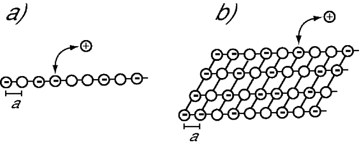
Figure 26: Schematic representation of the geometry used in the charge-regulation mean-field theory. a) A straight polyelectrolyte chain consists of $N$ dissociable monomers which can be either charged or neutral. b) A two-dimensional surface contains dissociable surface groups that are positioned on some regular lattice, here chosen to be a square lattice. The nearest-neighbor distance in both cases is $a$.

Let us first consider the case of a single charged polymer or polyelectrolyte (PE). In the present simplified model, we neglect conformational degrees of freedom of the PE and assume a straight polymer consisting of $N$ monomers with a bond length (i.e. distance between dissociable groups) $a$, as is depicted in Fig. 26a. This model is applicable to stiff PEs and for strongly adsorbed PEs, since they are indeed flat. The statistical mechanics of this problem is quite involved as it involves summation over all possible charge distributions on the line; the partition function reads

$$Z=\sum_{\{s_{i}\}=0,1}{\rm e}^{-{\cal H}}$$ (80)

where the Hamiltonian (in units of $k_{B}T$) is for monovalent monomers defined as

$${\cal H}=\mu\sum_{i}s_{i}+\sum_{i>j}s_{i}s_{j}v_{\rm DH}(a|i-j|)$$ (81)

and $s_{i}$ is a spin variable which is 1 (0) if the i-th monomer is charged (uncharged). The chemical potential for a charge on a monomer is given by

$$\mu=-2.303(pH-pK_{a})-\ell_{B}\kappa.$$ (82)

The first term is the chemical free energy gained by dissociation, which contains the chemical binding energy including Coulomb attraction between acidic rest and proton and also the concentration of protons as explained above; the second term is the sum of the self-energies of the released proton and the dissociated acid. The self-energy of a single charge follows from the expression

$$\lim_{r\rightarrow 0}\frac{v_{\rm DH}(r)-\ell_{B}/r}{2}=-\ell_{B}\kappa/2,$$ (83)

where the bare Coulomb self energy (which is a divergent constant) has been subtracted; it measures the free-energy gain associated with the build-up of the counterion cloud. It can be derived by integrating the electrostatic field energy over the entire space, or, which is simpler, by a thermodynamic charging procedure.

All different charge distributions are explicitly summed in Eq.(80), which together with the long-ranged interaction $v_{\rm DH}(r)$ between charged monomers makes the problem difficult. From the partition function, Eq.(80), one derives the rescaled free energy per monomer, $f=-\ln(Z)/N$, from which the fraction of charged monomers is obtained as $\alpha=\partial f/\partial\mu$. Previously, similar problems have been solved using continuous mean-field theory[250, 254, 255], restriction to only nearest-neighbor repulsions[256, 257, 258, 259] and computer simulations[260, 261]. In the presence of long-ranged charge repulsions, however, nearest-neighbor approximations break down, while the continuous mean-field theories neglect the short-range structure of the charged species (they do not know about the minimal distance between dissociable sites). Simulations provide accurate and specific answers, but for practical purposes a closed-form solution in terms of a formula is desirable. Lattice mean-field theory provides a simple close-form solution to the problem; the accuracy of this approach has been demonstrated by extensive comparison with exact enumerations [253] . To proceed, one defines a variational Hamiltonian which is chosen to be so simple that closed-form solution of the partition function is possible. Standard mean-field theory employs a single-site Hamiltonian of the form

$${\cal H}_{0}=h\sum_{i}s_{i}$$ (84)

with $h$ being an as yet undetermined variational parameter. The variational free energy is defined as

$$f_{var}=f_{0}+\langle{\cal H}-{\cal H}_{0}\rangle_{0}$$ (85)

where $f_{0}=-\ln(1-e^{-h})$ is the free energy per site of the variational Hamiltonian. All expectation values appearing in the variational free energy can be explicitly calculated. Due to its construction, the variational Hamiltonian is a strict upper bound to the true free energy, i.e. $f_{var}\geq f$, and therefore the best possible estimate of the true free energy is reached by minimizing $f_{var}(h)$ with respect to the variational parameter $h$. The resultant free energy $f_{MF}=\min_{h}f_{var}(h)$ is the mean-field approximation, from which the mean-field dissociation degree $\alpha$ can be calculated via the already presented formula $\alpha=\partial f_{MF}/\partial\mu$. The resultant expression has been extensively compared with exact enumeration studies and found to be very accurate, especially at low salt concentration[253]. The result can be given as an implicit expression,

$$-\mu=2.303(pH-pK_{a})+\ell_{B}\kappa=\ln\frac{\alpha}{1-\alpha}+\Delta\alpha$$ (86)

which can numerically or graphically be inverted. Here,

$$\Delta=2\sum_{n=1}^{\infty}v_{DH}(na)=\frac{2\ell_{B}}{a}\sum_{n=1}^{\infty}\frac{e^{-a\kappa n}}{n}=-2(\ell_{B}/a)\ln(1-e^{-\kappa a})$$ (87)

is the charge regulation parameter which takes charge-repulsion between neighboring monomers into account. It has the limiting behavior $\Delta\simeq-2(\ell_{B}/a)\ln(\kappa a)$ for $\kappa a\rightarrow 0$ and $\Delta\simeq 2(\ell_{B}/a)e^{-\kappa a}$ for $\kappa a\gg 1$. For $\Delta=0$ (obtained for large salt concentration $\kappa a\gg 1$) the usual ’law-of-mass-action’ dissociation behavior is obtained, for $\Delta>0$ the dissociation is much reduced. It is interesting to compare our result Eq.(86) with previous heuristic formulas which include the effects of charge repulsion on the dissociation by phenomenological fitting parameters[262, 263]. Our expression is different, but in fact not more complicated.

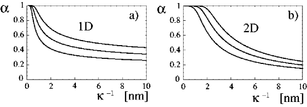
Figure 27: a) Mean-field results for the dissociation fraction $\alpha$ of a poly-anion in the bulk with monomer separation $a=0.25nm$ for fixed $pH-pK_{a}=2,3,4$ (from bottom to top) as a function of the screening length $\kappa^{-1}$. b) Dissociation fraction of charge groups on a surface with lateral group separation of $a=1nm$ for fixed $pH-pK_{a}=2,3,4$ (from bottom to top) as a function of the screening length $\kappa^{-1}$.

In Fig.27a the fraction of charged monomers is presented for a polyacid with monomer-separation $a=0.25nm$, as applicable to vinyl-based polymers, for fixed $pH-pK_{a}=2,3,4$ (from bottom to top) as function of the screening length in the bulk. As is well known, the dissociation for all but very high salt concentrations (small $\kappa^{-1}$) is incomplete and further decreases with increasing $\kappa^{-1}$, a phenomenon called charge regulation. As a main result, even rather strong PEs are only partially charged at low salt concentrations[250] (where we have not taken additional complications due to chemical binding of metal ions into account[258, 264]).

On a two-dimensional surface, the mean-field formalism works just as well. The only modification concerns the charge regulation parameter $\Delta$, which now takes interactions of one charge with all neighbors in two dimensions into account. Assuming the dissociable sites to be located on a 2D square lattice with lattice constant $a$, as schematically depicted in Fig.26b, it is given by

$$\Delta=\sum_{n=-\infty}^{\infty}\sum_{m=-\infty}^{\infty}v_{DH}(\sqrt{m^{2}+n^{2}}a)=\frac{\ell_{B}}{a}\sum_{n=-\infty}^{\infty}\sum_{m=-\infty}^{\infty}\frac{e^{-a\kappa\sqrt{m^{2}+n^{2}}}}{\sqrt{m^{2}+n^{2}}}.$$ (88)

In contrast to the one-dimensional case, the double sum (where the origin is excluded) cannot be performed exactly. Since we are mostly interested in the behavior when the screening length is large, we can use the isotropic form of the summand and make the simplification $\sum_{n=-\infty}^{\infty}\sum_{m=-\infty}^{\infty}\approx 2\pi\sum_{n=1}^{\infty}$ and obtain the result

$$\Delta=\frac{2\pi\ell_{B}}{a}\frac{1}{e^{\kappa a}-1}$$ (89)

with the limits $\Delta\simeq 2\pi\ell_{B}/(\kappa a^{2})$ for low salt $\kappa a\rightarrow 0$ and $\Delta\simeq 2\pi\ell_{B}e^{-\kappa a}/a$ for high salt $\kappa a\gg 1$. The main difference to the 1D case is the behavior for small salt concentrations or large screening lengths, where the coupling is much larger and thus the dissociation is even further reduced as compared to the 1D case. This is demonstrated in Fig.27b, where we show the dissociation fraction of charge groups, $\alpha$, on a surface as a function of the screening length $\kappa^{-1}$ for fixed $pH-pK_{a}=2,3,4$ (from bottom to top) . We chose a lateral surface group separation of $a=1nm$ which is much larger than the charge distance for the polymer in Fig.27a, which reflects that surface charges are typically more sparse than charges on polyelectrolytes. Still, the surface dissociation is highly reduced, especially for large screening lengths where the interaction between groups that are distant comes into play. Comparing the 1D and 2D case one indeed sees that on the surface the dissociation degree drops faster as the screening lengths increases, which has to do with the functional dependence of the charge regulation parameter $\Delta$ on $\kappa a$ (inverse power law in 2D as opposed to logarithmic in 1D).

In summary, charge regulation happens and reduces the charge of all objects with dissociable surface groups, especially at low salt concentrations. It should be taken into account especially when interactions between charged objects are considered. In MD simulations of weakly acidic groups, force fields have to be used which take the chemical binding effects into account. Quantum-chemistry methods can be of help, as they allow to determine those chemical binding forces, as will be explained in Section 11.

10 Water at hydrophobic substrates

In the simplified models used in the previous sections the presence of water was accounted for only by the presence of a uniform relative dielectric constant with the value $\varepsilon=78$. As is routinely done in most theoretical considerations, no other water effects were included, which works for many cases, but especially at surfaces is a highly questionable concept, as will be discussed now. For very large non-polar objects or in the limiting case of a planar hydrophobic substrate in contact with water, it is known since a long time that the water density is reduced at the hydrophobic surface and the structure of the interfacial water is very different from the bulk[265, 266, 267]. Clearly, this has important consequences for all material constants characterizing the solution (dielectric constant, viscosity, screening length, $pK_{a}$) close to the surface. It seems fair to say that without a proper characterization of the behavior of water at hydrophobic surfaces, no true understanding of the properties of such surfaces and their interactions will be possible. Quite possibly, many of the features interpreted as being inherent to surfaces themselves, might in fact reflect properties of the interfacial water layer instead (e.g. protein adsorption resistivity[268], zeta potentials[269], surface potentials[270], polymer-adsorption energies[271, 272], just to mention a few). We will now consider the water density profile close to a planar surface using Molecular Dynamics (MD) simulations. In MD, one basically integrates Newton’s equation of motion for an assembly of molecules or atoms, using heuristically chosen force parameterizations. The constant pressure ensemble is realized by adjusting the system volume. For simplicity, we only consider neutral walls, and in order to bring out the consequences of the presence of a wall most clearly, we deal with the special case of a very hydrophobic wall.

The work described here was motivated by recent scattering experiments where the water density depletion at planar non-polar substrates was determined. As the main result of those experiments, it was shown that the effective depletion thickness (defined as the thickness of a step-like depletion layer consisting of vacuum with the same integrated depleted amount as the rounded and smeared-out depletion profiles found in experiments) is roughly 2.5 Angstroms on hydrophobic poly-styrene substrates[273] and 5 Angstroms on hydrophobic self-assembled monolayers[274] using neutron reflectivity methods, and about 1 Angstrom on paraffin substrates using X-ray reflectivity measurements[275]. The reason for the discrepancies among different experiments is not well understood, but since the strength of water depletion is reduced with decreasing radius of curvature of the hydrophobic solutes[276], it is clear that surface roughness is one important factor (among many others, as e.g. small traces of attractive interactions between wall and water molecules) and will, if present, reduce the depleted amount.

In the simulations, we built up the hydrophobic substrate by self assembled alkane chains which seems to be an acceptable representation of the substrate structure used in recent experiments[273, 274, 275]. In Figure 28a) a snapshot of the MD simulation is shown, which serves to illustrate the geometry of the system[276]. The alkane molecules form a compact slab in the middle of the simulation box. They are only allowed to fluctuate in the z-direction and thus allow for fast pressure equilibration. The water slab has a thickness of about 4 Nanometers, which should be large enough such that bulk water properties are reproduced. We therefore interpret our results as being caused by the single hydrophobic substrate – water interface and neglect interactions between the two interfaces through the finite water slab.

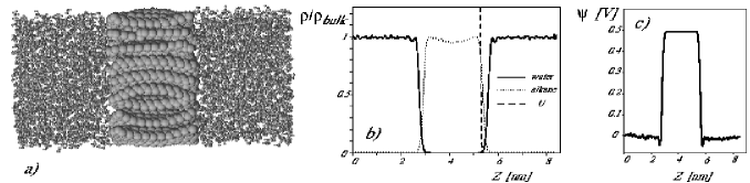
Figure 28: a) Snapshot of the MD simulation of a planar hydrophobic slab (made up of 64 alkane molecules) in contact with a water slab, consisting of 2781 SPC/E water molecules. b) Normalized density profile of the hydrophobic alkane slab (dotted line, in the middle) and the water layers (solid line, to the left and to the right) at constant pressure of 1 bar and temperature T=300K. The broken line denotes $U(z)$, the laterally averaged Lenard-Jones potential felt by the water molecules in units of $k_{B}T$. The system was thermalised for 100 ps and averaged for 2 ns. c) Local electrostatic potential across the water-alkane interface, exhibiting a potential drop of about 0.5 Volts.

In Figure 28b) we show the normalized densities of the alkane slab (dotted line) and the water layer (solid line) at atmospheric pressure and at a temperature T=300K. It is clearly seen that between the alkane slab and the water layer a region of reduced density appears. The density profiles are calculated using point-like atomic form factors and denote the nuclear density; they therefore correspond to what would be seen in a neutron scattering experiment. The broken line denotes the laterally averaged interaction potential due to the alkane slab, in other words, this is the potential energy felt by the water molecules. At room temperature and normal pressure, we obtain for the depletion thickness of a planar hydrophobic substrate the value $d_{2}=2.565$ Å, which is of the order of the length obtained in recent neutron scattering experiments[273, 274] and twice the length obtained with X-rays at hydrophobic substrates[275]. In Fig. 28c the electrostatic potential across the interface is shown to change by about 0.5 V, which is due to the almost complete orientation of the topmost water layer.

What do these results imply for charged surfaces? Many of the charged surfaces used in experiments are in fact, if one forgets about the charged groups for a moment, of hydrophobic nature. Let us assume for the sake of argument that the hydrophobic effects discussed above persist, even when charges are present. A layer of reduced water density at such surfaces means that the effective dielectric constant is reduced; this suggests that i) the association-dissociation equilibrium of surface charges is perturbed and ii) that electrostatic interactions at hydrophobic surfaces in general might be stronger than anticipated based on simpler models. The viscosity at the surface will most likely be reduced which might be important in connection with electrokinetic effects. Finally, the polarity of the top water layer is such that in principle (i.e. neglecting ion-water interactions) negative ions should be preferentially adsorbed on the surface. This is indeed borne out by recent MD simulations[277], which however demonstrated an additional subtle dependence on the presence of ionic polarizabilities. For interactions between charged surfaces it is conceivable that the hydrophobic attraction due to the overlap of the depletion layers might very well dominate the resulting behavior.

11 Ion-specific effects

In the preceding sections, ions were either treated as point-like or as hard spheres. However, as has been recently reviewed[31, 278], a large number of phenomena in colloid, polymer, and interface science that involve electrolytes show pronounced ion-specificity, as categorized in the famous Hofmeister series[279, 280, 281, 282, 283]. A striking experimental example of counterion specificity is obtained for the cationic surfactant discussed in Section 3. Exchanging the Bromine ion in DDAB by a Chlorine ion, the phase diagram changes dramatically and the phase coexistence disappears completely[40]. A subset of these unresolved issues is typically associated with the so-called hydrophobic force, a rather long-ranged attraction between hydrophobic surfaces, which is much stronger than predicted from standard van-der-Waals calculations and is also strongly ion-type-dependent[284]. Previous theoretical explanations invoked solvent-structure effects[285, 286, 287, 288, 289], and surface-specific ion interactions[290, 291] or charge-regulation phenomena[292]. The presence of excess ionic polarizabilities was proposed to lead to corrections to the usual van-der-Waals interaction energy, which could be one of the factors determining ion-specific interactions[293, 294, 295, 296]. But it was also shown that even with pure Coulomb interactions, one obtains strong deviations from the standard mean-field approaches if one takes into account that the charge distribution on all charged surfaces is laterally modulated[54, 124, 125, 127, 128]. Specifically, the counterion density right at a charged surface (which for a homogeneously charged surface and in the absence of additional interactions is exactly given by Eq.(15) because of the contact-value theorem) is for a modulated surface charge distribution increased. Surface-charge inhomogeneities in that sense act like additional attractive interactions between surfaces and ions, but it should be clear that all the above-mentioned effects are present simultaneously. It is therefore not easy to disentangle these various factors, especially since experimentally one typically measures macroscopic quantities such as surface tension, ionic activities, ionic osmotic coefficients, etc. and not ionic distribution functions from which effective interactions between ions and surfaces could be deduced. As an additional complication, computer simulations, which would include all above mentioned effects, are still difficult to perform, even using coarse-grained models where one replaces explicit solvent by some suitably chosen dielectric constant plus solvent-induced effective interactions between solute molecules. One therefore has to rely on various approximations, and it is often not easy to tell to what degree the approximation or the model parameters are responsible for the outcome.

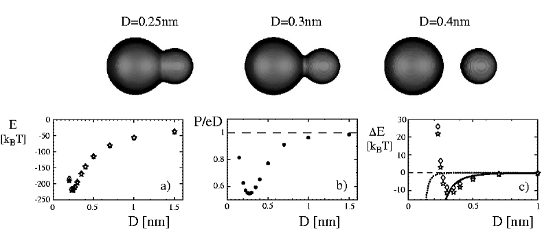
Figure 29: Top panel: Surfaces of constant electron density (roughly corresponding to the density at the Pauling surface) for three different values of the distance $D$ between a sodium (to the right) and a chloride ion (to the left) in vacuum. a) Interaction energy obtained using Hartree-Fock with a TZV basis set (open diamonds) and including electron-correlations on the MP2 level (open stars). b) Dipole moment divided by distance as a function of the ion distance, indicating that the two ions are fully charged for large separations. c) Non-coulombic interaction obtained by subtracting the Coulomb energy from the data in a). Note that a deep minimum is present which can be explained by the charge-induced dipole interaction (solid line) for large distances. The dispersion interaction (dotted line) is irrelevant for all distances. All data are obtained in vacuum.

How do we expect ion-specific effects to come into play on a microscopic level? At any charged surface, one has chemical groups which carry most of the surface charge, i.e., at which location the charge density is locally increased. The counterions (or any other oppositely charged molecule) will, due to Coulomb interactions, be on average quite close to these surface groups (in fact much closer than would be predicted according to Poisson-Boltzmann theory assuming a laterally homogeneous surface charge, compare Section 4), and it seems natural to surmise that it is the interaction between oppositely charged chemical groups that will be most susceptible to chemical specificity. This is not to say that solvent effects (i.e. water structuring which of course is different for different ion types) is unimportant, on the contrary, but it does not make sense to separate solvent-induced effects from the bare interactions between oppositely charged groups. One experimental example where the specificity is exhibited very clearly is with AFM experiments for polyelectrolytes adsorbed on a variety of different substrates and in different electrolyte solutions[271, 272], where the plateau desorption force can be directly converted into the binding energy per unit length.

11.1 Interactions between ions

Fortunately, progress in the available quantum-computational methodology allows to calculate effective interactions between charged species in an essentially ab-initio manner[297], including solvent effects[298]. As a prototype for the effects studied, we show in Fig.29 ab-initio results for the interaction between a sodium and a chloride ion in vacuum. In Fig.29a we show the resulting interaction energy between the two ions as a function of their mutual distance in units of $k_{B}T$. The open diamonds are obtained using Hartree-Fock (HF) methods, i.e. each electron sees a mean-charge-distribution due to the other electrons, otherwise the Schrödinger equation is explicitly solved for all 28 electrons involved (treating the nuclei as being fixed), using an expansion in TZV basis functions with added polarization and diffuse wave functions. The open stars denote results where electron correlations have been taken into account on the one-loop level (HF-MP2), the energy is slightly lower. One would expect that most of the long-ranged attraction seen in Fig.29a is due to the Coulomb attraction between the separated charges on the two ions. To make that notion quantitative, we first have to find out how much charge is transferred between the two ions. In Fig.29b we plot the ratio of the dipole moment of the whole charge distribution (including both ions and in units of the elementary charge) and the ion-ion separation as a function of the separation. This ratio can be interpreted as the effective charge transfered between the two ions. It is seen that indeed charge transfer is almost perfect at large distances in which limit both ions are fully charged. For smaller distances polarization effects lead to a decrease of the transfered charge. In Fig.29c we show the same data as in Fig.29a but with the Coulomb attraction $v(r)=-\ell_{B}/r$ subtracted (note that the Bjerrum length in vacuum measures $\ell_{B}=55.73nm$). Quite surprisingly, the resulting energy shows a pronounced attractive minimum of depth $\simeq-10k_{B}T$ in a distance range $0.25nm<D<0.4nm$. Both HF and MP2 calculations give roughly the same result, the difference between the two can be viewed as an estimate for the systematic error in the calculation (an additional source of error is introduced due to the necessarily incomplete basis sets used). What is the reason for this quite strong attraction between the ions? To the mind come two contributions, namely the polarization attraction due to the charge-induced dipole interaction and the van-der-Waals interaction. Let us discuss both in some detail.

The static polarizability of the isolated ions can be calculated using the same ab-initio methods by applying a small electric field and measuring the induced dipole moment (or by measuring the polarization energy). We obtain $\alpha_{Cl^{-}}/(4\pi\varepsilon_{0})=3.404$ ų within HF and $\alpha_{Cl^{-}}/(4\pi\varepsilon_{0})=3.666$ ų within HF-MP2 for the $Cl^{-}$ ion and $\alpha_{Na^{+}}/(4\pi\varepsilon_{0})=0.132$ ų within HF and $\alpha_{Na^{+}}/(4\pi\varepsilon_{0})=0.143$ ų within HF-MP2 for the $Na^{+}$ ion. Other data are collected in Table 1. The charge-induced dipole interaction between the $Cl^{-}$ and $Na^{+}$ ions is in units of $k_{B}T$ [299]

$$w_{\rm ind}(r)=-\frac{\ell_{B}(\alpha_{Cl^{-}}+\alpha_{Na^{+}})}{8\pi\varepsilon_{0}r^{4}}$$ (90)

and is plotted in Fig.29c as a solid line. It describes the ion-ion interaction quite well except for very small distances where the electron clouds overlap strongly. So it seems fair to say that corrections to the bare Coulomb interaction between ions in vacuum (which has been subtracted off in Fig.29c) are at large distances mostly dominated by polarization effects.

The dispersion interaction between two atoms has been calculated using quantum-mechanical perturbation theory[300, 301] and is given by (in units of $k_{B}T$)

$$w_{\rm disp}(r)=-\frac{3\alpha_{Cl^{-}}\alpha_{Na^{+}}I_{Cl^{-}}I_{Na^{+}}}{2(4\pi\varepsilon_{0})^{2}(I_{Cl^{-}}+I_{Na^{+}})r^{6}}$$ (91)

where the ionization energies $I$ of the two ions are measured in units of $k_{B}T$ also. For the ionization potentials we obtain using the same level of HF-MP2 the results $I_{Cl^{-}}=138.57k_{B}T$ and $I_{Na^{+}}=1820.2k_{B}T$, other data can be found in Table 1. The resulting dispersion interaction is plotted in Fig.29c as a dotted line. It is basically negligibe for the whole relevant range of distances. This tells us that the attraction that appears in the quantum-mechanical calculation is at large distances mostly due to polarization effects. It has to be considered as an important factor in the interaction between charged surfaces, since such additional interactions between ions and surfaces lead to charge regulation and thus to varying effective surface charges[270]. Likewise, the interaction between ions in the bulk modifies the osmotic coefficients, the screening length, ionic activities and therefore gives an additional shift of the surface-group dissociation equilibrium. Clearly, this interaction is highly specific and different for different ion types, especially at small distances. A hand-waving explanation why the very short-ranged properties of this interaction will be important is that oppositely charged ions are squeezed together such that the electron orbitals overlap to a degree where quantum-mechanical effects come into play. This might be intuitively understood by looking at the electron-density contours shown in the upper panel in Fig.29. In all three pictures, the electron densities on the contour surfaces are the same and roughly correspond to the density on the Pauling surfaces (the Pauling ionic radius as deduced from crystal structures for the $Cl^{-}$ ion is $R_{Cl^{-}}\simeq 0.181nm$ and for the $Na^{+}$ ion it is $R_{Na^{+}}\simeq 0.095nm$). It is seen that for the range of distances where the attraction is strongest the electron distributions overlap. A similar short-ranged interaction between ions had been introduced in an ad-hoc fashion in order to accurately fit activity coefficients of alkali-halide solutions[302, 303], but we argue here that it is a general feature of oppositely charged groups and not restricted to simple ions but also applies to the interaction between macroscopic charged bodies. A similar interaction should also be present for the case of similarly charged ions, though here we would in general expect the effects to be small since the Coulomb repulsion in this case will make close contacts between ions unlikely in the general case. In previous theories which concentrated on water-structure effects for electrolyte behavior, the bare interionic potential has been typically regarded as rather structureless[288]. It might be interesting to reconsider such calculations by adding quantum-mechanical potentials as we have calculated.

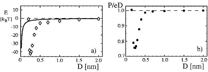
Figure 30: a) Interaction energy between a sodium and a chloride ion using Hartree-Fock methods and a polarizable continuum model with parameters representing liquid water. Open diamonds represent the full interaction energy in units of $k_{B}T$. The solid line corresponds to the Coulomb interaction between two unit charges in a homogenous material of relative dielectric constant of $\varepsilon=78.39$, which underestimates the true attraction considerably. b) Dipole moment divided by distance as a function of the ion distance, indicating that the two ions are fully charged already for intermediate separations.

Table 1: Ab-initio results for ionization energies $E_{ion}$ and polarizabilities $\alpha$ for various atoms and ions in vacuum. The cavity radii $R_{cav}$ are by a factor 1.2 larger than the Pauling radii. The effective ionic dielectric constant $\varepsilon$ and the excess polarizabilities $\alpha_{exc}^{\infty}$ at large frequencies and at zero frequency $\alpha_{exc}^{0}$ are calculated from the Clausius-Mossotti/Lorenz-Lorentz equation, see text. The shift of the ionization energy in water, $\Delta E_{ion}$, is calculated using a simple Born self-energy model. For conversion, note that $1eV=96.4516kJ/mol$ and $1eV=38.610k_{B}T$. Numbers in parantheses are experimental values.

	$E_{ion}$ [eV]	$\frac{\alpha}{4\pi\varepsilon_{0}}$ [Å3]	$R_{cav}$ [Å]	$\varepsilon$	$\frac{\alpha_{exc}^{\infty}}{4\pi\varepsilon_{0}}$ [Å3]	$\frac{\alpha_{exc}^{0}}{4\pi\varepsilon_{0}}$ [Å3]	$\Delta E_{ion}$ [eV]
$Li$	5.37 (5.39)	24.9 (24.3)
$Li^{+}$	75.0	0.022	0.72	1.186	-0.040	-0.18	- 29.7
$Na^{+}$	47.1	0.14	1.14	1.32	-0.11	-0.72	-18.8
$K^{+}$	31.5	0.81	1.596	1.75	0.062	-1.97	-13.4
$Fl^{-}$	3.54	1.01	1.632	1.90	0.195	-2.10	4.37
$Cl^{-}$	3.59	3.67	2.172	2.62	1.63	-4.87	3.28
$Br$	13.6 (11.81)	2.91 (3.05)
$Br^{-}$	3.39	6.61	2.34	4.19	4.29	-5.91	3.04
$NO_{3}^{-}$	3.69	4.69	2.45	2.40	1.88	-7.04	2.91
$SCN^{-}$	2.42	7.48	2.62	3.14	4.08	-8.45	2.72
$H_{2}O$		1.31 (1.45)	1.93	1.669 (1.78)

Conversely, it is important within our approach to critically check how the interaction we obtain will be modified in the presence of water. To do so we performed Hartree-Fock calculations using the so-called polarizable-continuum-model where the ions are embedded in spherical shells outside of which a dielectric medium with relative dielectric constant $\varepsilon=78.39$ is assumed. The choice of the radii of these cavities is critical, we chose the cavity radii to be bigger than the Pauling radii of the ions by a factor 1.2. This means that the two dielectric cavities for the case of $Na^{+}$ and $Cl^{-}$ start touching at a distance of $D=1.2(0.095nm+0.181nm)=0.331nm$. The Schrödinger equation is then solved taking into account the effects of polarization charges[298]. The open diamonds in Fig.30a represent the full interaction obtained between the two ions. One notes that the long-ranged attractive tail has almost disappeared. The solid line corresponds to the Coulomb interaction between two unit charges with a relative dielectric constant of $\varepsilon=78.39$. This Coulomb potential is quite small, which is understandable since the Bjerrum length now takes the value $\ell_{B}\simeq 0.71nm$. It is important to note that the true electrostatic interaction is quite involved because of the complicated geometry: for distances larger than $D=0.331nm$ one has two separate spherical dielectric cavities which are immersed in a high-dielectric background mimicking water. For smaller distances, the spherical cavities overlap. The Coulomb interaction between two charges inside the cavities shows a complicated crossover from a weak interaction at large distances, characterized by a Bjerrum length $\ell_{B}\simeq 0.71nm$, to a strong interaction at distances smaller than the cavity-overlap distance, where the Bjerrum length becomes closer to the vacuum value $\ell_{B}=55.73nm$. This is more or less what one sees in the data in Fig.30a. As a consequence, the short-ranged attraction is even stronger and now has a depth of $40k_{B}T$. It should be noted that this short-ranged attraction is mostly due to the modification of the Coulomb potential in the presence of dielectric boundaries (for similarly charged ions, the effective interaction will be predominantly repulsive).

What would we expect for the charge-induced-dipole and the dispersion interaction in this case? To make progress we first need to evaluate the effective dielectric constant of the ion-containing cavity, which follows from the Clausius-Mossotti equation[33] (or the frequency-dependent analogue, the Lorenz-Lorentz equation[32]) by

$$\varepsilon=\frac{2\alpha/(4\pi\varepsilon_{0}R^{3})+1}{1-\alpha/(4\pi\varepsilon_{0}R^{3})}.$$ (92)

For the chloride ion with $R_{Cl^{-}}\simeq 0.2172nm$ and $\alpha_{Cl^{-}}/(4\pi\varepsilon_{0})=3.666\AA^{3}$ one obtains $\varepsilon_{Cl^{-}}\simeq 2.62$ and for the sodium ion with $R_{Na^{+}}\simeq 0.114nm$ and $\alpha_{Na^{+}}/(4\pi\varepsilon_{0})=0.143\AA^{3}$ one obtains $\varepsilon_{Na^{+}}\simeq 1.32$, where these numbers are equally valid in the static and dynamic case. Other results for different atoms and ions are given in Table 1. For the charge-induced dipole interaction what counts is the static excess polarizability of the ions in water, which again can be calculated from the inverted Clausius-Mosotti/Lorenz-Lorentz equation,

$$\alpha_{exc}/(4\pi\varepsilon_{0})=R^{3}\frac{\varepsilon_{ion}-\varepsilon_{water}}{\varepsilon_{ion}+2\varepsilon_{water}}$$ (93)

and is denoted by $\alpha^{0}_{exc}$ and given in Table 1. Since water has a much higher static dielectric constant than the ions, $\varepsilon_{water}^{0}=78.39$, it is clear that the excess static polarizability is negative and thus the charge-induced dipole contribution to the interaction energy is repulsive. It is therefore ruled out as a possible explanation for the observed attraction between the ions seen in the data in Fig.30a. For the dispersion interaction we have a static contribution, which is attractive but rather weak (since it is at most of the order of $3k_{B}T$ at contact[299]) and a dynamic contribution. For the dynamic dispersion interaction what counts is the frequency-dependent dielectric constant of the ions, given above, and of water, which follows from the refractive index $n\simeq 1.33$ as $\varepsilon_{water}^{\infty}=n^{2}\simeq 1.78$. According to the Lorenz-Lorentz equation (93), the excess polarizability is reduced, such that the dynamic dispersion interaction will be even smaller than the one in vacuum (which is shown in Fig.29c as a dotted line). To get explicit numbers for the dynamic excess polarizabilities of ions in water, we have calculated the high-frequency dielectric constant of water within our ab-initio technique using the same method as for the ions. The result is $\varepsilon^{\infty}_{water}=1.669$ and thus smaller than the experimental value by 10 % (see Table 1). For consistency reasons, we have estimated the finite-frequency ion excess polarizabilities with the calculated value of the water dielectric constant. The results are given in Table 1. The resulting excess polarizabilities are always smaller than the ones in vacuum. We also estimate the ionization energies in the water environment using a simple Born self-energy argument. For the anion, the ionization energy is increased by the term

$$\Delta E_{ion}=(\ell_{B}^{vac}-\ell_{B}^{water})/(2R_{cav})$$ (94)

which measures the electrostatic self-energy difference of a charged sphere in vacuum and in water. The vacuum Bjerrum length is given by $\ell_{B}^{vac}=55.73nm$ and the Bjerrum length in water is $\ell_{B}^{water}=0.71nm$. For the cations, the ionization energy is reduced by the term

$$\Delta E_{ion}=-(4-1)(\ell_{B}^{vac}-\ell_{B}^{water})/(2R_{cav})$$ (95)

which is the self-energy difference of a divalent and a monovalent charged sphere in vacuum and in water. The resulting numerical values are given in Table 1. The effect of the ionization energy change on the dispersion interaction is roughly to increase the dispersion strength by a factor of two (this follows from the fact that the sum of ionization energies in the denominator of equation (91) is dominated by the larger cationic energy which therefore cancels the cationic energy in the numerator). The reduction of the polarizability in water however is larger than the increase of the ionization term, so that in essence the dispersion interaction in water is even weaker than in vacuum. Similarly to the situation in vacuum, therefore, the dispersion interaction is only a negligible contribution to the full interaction obtained within the ab-initio calculation. As a main result, we find that, owing to the shape and size dependent crossover of the effective Coulomb interaction, the effective interaction between ions in a polarizable continuum medium is thus quite specific and depends sensitively on the shape and size of the ions. It remains to be checked how these results will be modified if discrete water molecules are included in the calculation, but it seems likely that specific short-ranged interactions between oppositely charged chemical groups play an important role in the physics of strongly charged systems.

11.2 Dissociation constants

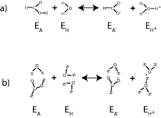
Figure 31: Dissociation reaction of a carboxylic acid, in a) without bound water and in b) with one associated water molecule. In the PCM calculations a cavity is formed consisting of spheres centered at the heavy atoms. Outside the cavity the dielectric constant is that of water, inside it takes the vacuum value.

The dissociation of an acid is a special case of the interaction between two oppositely charged ions, namely the acidic rest group and the proton. We will specifically consider the dissociation of the carboxylic acid, which has been quite extensively studied in the literature and serves as a good model to compare different approaches with each other[304, 305, 306]. The basic chemical reaction, according to the formula Eq.(76), is depicted in Fig.31a. In the quantum chemical calculation we optimize the conformation of each ’molecule’ and calculate the energy in the electronic and conformational ground state. The results for all energies for a vacuum calculation of reaction a) are given in the first row in Table 2. All energies are expressed in units of $k_{B}T$. The actual numbers are quite large, since all core electrons contribute. It is clear that in order to extract the binding energy of the proton, high precision is needed since we are interested in the small difference between large numbers. We define the energy differences $\Delta E_{A}=E_{A-}-E_{A}$ and $\Delta E_{H}=E_{H+}-E_{H}$, from which the binding energy is obtained as $\Delta E=\Delta E_{A}+\Delta E_{H}$. According to Eq.(78) the acidic dissociation constant is

$$K_{a}=e^{-\Delta E}[H_{2}O],$$ (96)

or, after taking the negative common logarithm and using that the water concentration is roughly $[H_{2}O]=55mol/l$,

$$pK_{a}=\frac{\Delta E}{2.303}-1.74.$$ (97)

The $pK_{a}$ that comes out from the vacuum calculation is $pK_{a}=122$ and disagrees wildly with the experimental value $pK_{a}=3.77$ for carboxylic acid[304, 305, 306]. The deviation is caused by the neglect of the surrounding water, which tends to support the dissociation reaction (and thus lowers the $pK_{a}$ value). In the second row we show the reaction b) pictured in Fig.31, which involves one coordinated water molecule but otherwise occurs in vacuum. The $pK_{a}$ is lowered down to $pK_{a}=92.7$ but is still much too high. Building larger and larger water clusters is possible, but not entirely satisfactory because the orientational freedom of liquid water is not preserved in a zero-temperature quantum-chemistry calculation. As already described in Section 11.1, the dieletric properties of water can be approximately taken into account by enclosing all molecules in a cavity outside of which a dielectric medium is present. The free parameter here is the radius of the cavity, which consists of spheres that are centered around all heavy atoms. In the next four rows in Table 2 we show a set of results where the ratio between the Pauling radii of the ions and the cavity radius is changed from 1.2 (the standard value) down to 0.9. It is seen that a smaller cavity radius brings down the $pK_{a}$ value, until finally for a ratio of 0.9 a result close to the experimental value $pK_{a}\approx 3.77$ is found. In a previous calculation a similar problem of obtaining agreement between experimental $pK_{a}$ values and calculated ones was detected and discussed at length[306]. In a sense, we use the cavity radius factor as an adjustable parameter to reproduce experimental results. It is important to note that we do not attach much physical significance to this adjustment and leave the whole problem of predicting $pK_{a}$ values to future investigations. Our heuristic viewpoint is utilized in the last row of Table 2, where we show a calculation where instead of the proton a sodium atom is allowed to bind to the carboxylic acid. As expected, the resultant value $pK_{a}=-7.5$ shows that sodium binding can totally be neglected. But for different acids and other ions the binding constants might well be such that chemical binding must be taken into account as a possible alternative to protonation events. One example includes the case of Calcium ion binding to polyacrylic acids[313].

Table 2: Ab-initio results for the ground-state energies involved in the dissociation of a carboxylic acid. The first two rows are for the reactions a) and b) in vacuum, as shown in Fig.31. The next four rows are for reaction a) but enclosed in a dielectric cavity, mimicking an aqueous environment. Here the cavity radius scaling factor is changed from 1.2 to 0.9. The last row contains results for the binding of a sodium ion. All energies are given in units of $kB_{T}$.

	$E_{A}$	$E_{A-}$	$\Delta E_{A}$	$E_{H}$	$E_{H+}$	$\Delta E_{H}$	$\Delta E$	$pK_{a}$
reaction a)	-198677	-198086	591.4	-80025.0	-80331.4	-306.4	285.0	122.0
reaction b)			578.9			-361.4	217.5	92.7
a) cavity 1.2			482.2			-430.8	51.4	20.6
a) cavity 1.1			477.1			-437.6	39.5	15.4
a) cavity 1.0			473.3			-445.4	28.0	10.4
a) cavity 0.9			471.9			-454.9	17.0	5.6
Na cavity 0.9							-13.1	-7.5

12 Summary and perspectives

A number of different situations have been reviewed which have in common that electrostatic effects play a dominant role. This is achieved for highly charged surfaces and for highly charged polymers. Among the most salient results we find simple explanations for the puzzling phenomena of attraction between similarly highly charged surfaces and overcompensation of charged surfaces by adsorbing polyelectrolytes. In general terms, it is the long-range nature of the Coulomb interaction which lies at the heart of these effects. We also briefly talk about the effect of electric fields on strongly coupled charged systems. For the specific case of a collapsed charged polymer, an electric field induces motion of ions and charged monomers and for high enough fields disolves the complex. This is an intrinsic non-equilibrium phenomenon. Finally, the interaction between oppositely charged chemical groups has been investigated using quantum-mechanical ab-initio methods. Since in highly charged systems one often has intimate contacts between such groups, the short-ranged bonding we find is quite relevant for the understanding of experiments where ion-specific effects are present. One has only started to bridge the gap between the quantum-mechanical world at small distances and the mesoscopic world of primitive models (where ions are replaced by hard spheres, and the solvent by a dielectric constant plus possibly effective interactions between the ions). What needs to be fully elucidated is the coupling between water structure close to ions and at charged surfaces and the effective interaction between such charged groups, which probably involves effective many-body interactions. Experimentally evidenced ion-specific effects will turn out to be a stringent test for such theories. Non-equilibrium phenomena are receiving more and more attention by theorists over the last years[314]. However, the whole field of electrophoresis and electroosmosis still contains many open questions. This is even more true for non-stationary non-equilibrium situations. Here simulation techniques are currently the method of choice, although field-theoretic and other analytical tools will prove useful as well.

References

- [1] Electrostatic Effects in Soft Matter and Biophysics, C. Holm, P. Kekicheff, und R. Podgornik (Eds.), Kluwer Academic Publishers, Dordrecht (2001).
- [2] P. Attard, in Advances in Chemical Physics, edited by I. Prigogine and S. A. Rice (John Wiley and Sons, New York, 1996), Vol. XCII.
- [3] J.P. Hansen and H. Löwen, Annu. Rev. Phys. Chem. 51 (2000) 209.
- [4] L. Belloni, J. Phys. Cond. Matter 12 (2000) R549.
- [5] Y. Levin, Rep. Progr. Phys 65 (2002) 1577.
- [6] A.Y. Grosberg, T.T. Nguyen, and B.I. Shklovskii, Rev. Mod. Phys. 74 (2002) 329.
- [7] P. Linse, J. Phys.: Condens. Matter 14 (2002) 13449.
- [8] A. Naji, S. Jungblut, A.G. Moreira, R.R. Netz, Physica A 352 (2005) 131.
- [9] J. Mahanty and B.W. Ninham, Dispersion Forces, Academic Press (London, 1976).
- [10] Verwey E.J.W.; Overbeek J.Th.G. Theory of the Stability of Lyophobic Colloids, Elsevier: Amsterdam, New York, 1948.
- [11] R.R. Netz, Phys. Rev. Lett. 76 (1996) 3646.
- [12] D.A. Weitz and J.S. Huang in Kinetics of Aggregation and Gelation, P. Family and D.P. Landau, eds. (Elsevier, Amsterdam, 1984).
- [13] D.H. Napper, Polymeric Stabilization of Colloidal Dispersions (Academic Press, London, 1983).
- [14] D. Horn, J. Rieger, Angew. Chem. Int. Ed. 40 (2001) 4330.
- [15] J. Rühe, M. Ballauff, M. Biesalski, P. Dziezok, F. Gröhn, D. Johannsmann, N. Houbenov, N. Hugenberg, R. Konradi, S. Minko, M. Motornov, R. R. Netz, M. Schmidt, C. Seidel, M. Stamm, T. Stephan, D. Usov, H. Zhang, Adv. Polym. Sci. 165 (2004) 79.
- [16] P.G. de Gennes, Scaling Concepts in Polymer Physics, (Cornell University, Ithaca, 1979).
- [17] M. Doi, S.F. Edwards, The Theory of Polymer Dynamics (Clarendon Press, Oxford, 1986).
- [18] A. Y. Grosberg and A. R. Khokhlov, Statistical Physics of Macromolecules ( AIP Press, Woodbury, N.Y., 1994).
- [19] Dautzenberg H.;Jaeger W.;Kötz B.P.J.;Seidel C.; Stscherbina D. Polyelectrolytes: Formation, characterization and application, Hanser Publishers: Munich, Vienna, New York, 1994.
- [20] S. Förster, M. Schmidt Adv. Polym. Sci. 120 (1995) 50.
- [21] J.-L. Barrat, J.-F. Joanny, Adv. Chem. Phys. 94 (1996) 1.
- [22] R.R. Netz, D. Andelman, Phys. Rep. 380 (2003) 1.
- [23] S. Schneider, P. Linse, Macromolecules 37 (2004) 3850.
- [24] T.D. Yager, C.T. McMurray, K.E. van Holde, Biochem. 28 (1989) 2271.
- [25] P. L. Dubin, M. E. Curran, and J. Hua, Langmuir 6 (1990) 707.
- [26] D. W. McQuigg, J. I. Kaplan, and P. L. Dubin, J. Phys. Chem. 96 (1992) 1973.
- [27] P. Haronska, T. A. Vilgis, R. Grottenmüller, and M. Schmidt, Macromol. Theor. Simul. 7 (1998) 241.
- [28] H. Zhang et al., J. Phys. Chem. B 103 (1999) 2347.
- [29] D.I. Gittins and F. Caruso, Adv. Mater. 12 (2000) 1947.
- [30] D.I. Gittins and F. Caruso, J. Phys. Chem. B 105 (2001) 6846.
- [31] W. Kunz, P. Lo Nostro, B.W. Ninham, Current Opinion Coll. & Interface Science, 9 (2004) 1.
- [32] C.J.F. Böttcher, Theory of Electric Polarization (Elsevier, Amsterdam, 1973).
- [33] P.F. Mossotti, Bibl. Univ. Modena 6 (1847) 193.
- [34] P.W. Debye, Phys. Z. 13 (1912) 97.
- [35] L. Onsager, J. Am. Chem. Soc. 58 (1936) 1486.
- [36] P.W. Debye and E. Hückel, Phys. Z. 24 (1923) 185.
- [37] M. Dubois and T. Zemb, Langmuir 7 (1991) 1352.
- [38] T. Zemb, L. Belloni, M. Dubois, and S. Marcelja, Progr. Colloids Polym. Sci. 89 (1992) 3.
- [39] T. Zemb, D. Gazeau, M. Dubois, and T. Gulik-Krzywicki, Europhys. Lett. 21 (1993) 759.
- [40] M. Dubois, T. Zemb, N. Fuller, R.P. Rand, and V.A. Parsegian, J. Chem. Phys. 108 (1998) 7855.
- [41] M. Dubois and T. Zemb, Curr. Opin. Coll. Interf. Sci. 5 (2000) 27.
- [42] B. Deme, M. Dubois, T. Gulik-Krzywicki, and T. Zemb, Langmuir 18 (2002) 997.
- [43] B. Deme, M. Dubois, and T. Zemb, Langmuir 18 (2002) 1005.
- [44] R. Lipowsky, in The Structure and Dynamics of Membranes, Handbook on Biological Physics, Vol. 1, Elsevier, Amsterdam (1995).
- [45] A. Khan, B. Jönsson, and H. Wennerström, J. Phys. Chem. 89 (1985) 5180.
- [46] H. Wennerström, A. Khan, and B. Lindman, Adv. Colloid Interface Sci. 34 (1991) 433.
- [47] I. Rouzina and V.A. Bloomfield, J. Phys. Chem. 100 (1996) 9977.
- [48] R.R. Netz, J.-F. Joanny, Macromolecules 32 (1999) 9013.
- [49] B. I. Shklovskii, Phys. Rev. E 60 (1999) 5802.
- [50] A. G. Moreira and R. R. Netz, Europhys. Lett. 52 (2000) 705.
- [51] A. G. Moreira and R. R. Netz, Phys. Rev. Lett. 87 (2001) 078301.
- [52] R. R. Netz, Eur. Phys. J. E 5 (2001) 557 .
- [53] A. G. Moreira and R. R. Netz, Eur. Phys. J. E 8 (2002) 33.
- [54] A.G. Moreira and R.R. Netz, Europhys. Lett. 57 (2002) 911.
- [55] M. Baus and J. Hansen, Phys. Rep. 59 (1980) 1.
- [56] D. Henderson and L. Blum, J. Chem. Phys. 69 (1978) 5441; D. Henderson, L. Blum, and J.L. Lebowitz, J. Electroanal. Chem. 102 (1979) 315; D. Henderson and L. Blum, J. Chem. Phys. 75 (1981) 2025.
- [57] S.L. Carnie and D.Y.C. Chan, J. Chem. Phys. 74 (1981) 1293.
- [58] H. Wennerström, B. Jönsson, and P. Linse, J. Chem. Phys. 76 (1982) 4665.
- [59] G. Gouy, J. de Phys. IX (1910) 457.
- [60] D. L. Chapman, Phil. Mag. 25 (1913) 475.
- [61] D. Andelman, in Handbook of Biological Physics, edited by R. Lipowsky and E. Sackmann (Elsevier, Amsterdam, 1995).
- [62] R.R. Netz and H. Orland, Eur. Phys. J. E 1 (2000) 203.
- [63] A.G. Moreira, R.R. Netz, in: Electrostatic Effects in Soft Matter and Biophysics, C. Holm, P. Kekicheff, und R. Podgornik (Eds.), (Kluwer Academic Publishers, Dordrecht 2001), p. 367.
- [64] Y. Burak, D. Andelman, H. Orland, Phys. Rev. E 70 (2004) 016102.
- [65] V. Garcia-Morales, J. Cervera, J. Pellicer, Physica A 339 (2004) 482.
- [66] C.D. Santangelo, to be published.
- [67] Y. Levin, J. Phys. Cond. Matter, 14 (2000) 2303.
- [68] R.R. Netz and H. Orland, Europhys. Lett. 45 (1999) 726.
- [69] L.M. Varela, M. Garcia, V. Mosquera, Phys. Rep. 382 (2003) 1.
- [70] Y.W. Kim, R.R. Netz, to be published.
- [71] L. Onsager, N.N.T. Samarras, J. Chem. Phys. 2 (1934) 528.
- [72] Y. Levin, J.E. Flores-Mena, Europhys. Lett. 56 (2001) 187.
- [73] R.R. Netz, Phys. Rev. E 60 (1999) 3174.
- [74] L. Guldbrand, B. Jönson, H. Wennerström, and P. Linse, J. Chem. Phys. 80 (1984) 2221.
- [75] D. Bratko, B. Jönsson, and H. Wennerström, Chem. Phys. Lett. 128 (1986) 449.
- [76] P. Kékicheff, S. Marčelja, T. J. Senden, and V. E. Shubin, J. Chem. Phys. 99 (1993) 6098.
- [77] J. Ray, G.S. Manning, Langmuir 10 (1994) 2450.
- [78] A.P. Lyubartsev, L. Nordenskiöld, J. Phys. Chem. 99 (1995) 10373.
- [79] N. Grønbech-Jensen, R.J. Mashl, R.F. Bruinsma, and W.M. Gelbart, Phys. Rev. Lett. 78 (1997) 2477.
- [80] B.-Y. Ha and A.J. Liu, Phys. Rev. Lett. 79 (1997) 1289.
- [81] R. Podgornik, V.A. Parsegian, Phys. Rev. Lett. 80 (1998) 1560.
- [82] A.P. Lyubartsev, J.X. Tang, P.A. Janmey, L. Nordenskiöld, Phys. Rev. Lett. 81 (1998) 5465.
- [83] Y. Levin, J.J. Arenzon, J.F. Stilck, Phys. Rev. Lett., 83 (1999) 2680 .
- [84] M.J. Stevens, Phys. Rev. Lett., 82 (1999) 101.
- [85] M. Deserno, A. Arnold, C. Holm, Macromolecules 36 (2003) 249.
- [86] A. Naji, A. Arnold, C. Holm, R.R. Netz, Europhys. Lett. 67 (2004) 130.
- [87] A. Naji, R.R. Netz, Eur. Phys. J. E 13 (2004) 43.
- [88] K.-C. Lee, I. Borukov, W.M. Gelbart, A.J. Liu, M.J. Stevens, Phys. Rev. Lett., 93 (2004) 128101.
- [89] E. Allahyarov, G. Gompper, H. Löwen, Phys. Rev. E 69 (2004) 041904.
- [90] F. Molnar, J. Rieger, Langmuir 21 (2005) 786.
- [91] E. Allahyarov, I.D’Amico, H. Löwen, Phys. Rev. Lett. 81 (1998) 1334.
- [92] Y. Levin, Physica A 265 (1999) 432.
- [93] P. Linse, V. Lobaskin, Phys. Rev. Lett. 83 (1999) 4208.
- [94] P. Linse, V. Lobaskin, J. Chem. Phys. 112 (2000) 3917.
- [95] P. Linse, J. Chem. Phys. 113 (2000) 4359.
- [96] R. Messina, C. Holm, K. Kremer, Phys. Rev. Lett. 85 (2000) 872.
- [97] V. Lobaskin, A. Lyubartsev, P. Linse, Phys. Rev. E 63 (2001) 020401 (R).
- [98] R. Messina, C. Holm, K. Kremer, Phys. Rev. E 64 (2001) 021405.
- [99] V. Lobaskin, K. Qamhieh, J. Phys. Chem. B 107 (2003) 8022.
- [100] W. Lin, P/ Galletto, M. Borkovec, Langmuir 20 (2004) 7465.
- [101] J. Ryden, M. Ullner, P. Linse, J. Chem. Phys. 123 (2005) 1.
- [102] G.M. Kepler and S. Fraden, Phys. Rev. Lett. 73 (1994) 356.
- [103] J.C. Crocker and D.G. Grier, Phys. Rev. Lett. 77 (1996) 1897.
- [104] A.E. Larsen and D.G. Grier, Nature 385 (1997) 231.
- [105] Y. Han, D.G. Grier, Phys. Rev. Lett. 91 (2003) 038302.
- [106] Jörg Baumgartl, Jose Luis Arauz-Lara, and Clemens Bechinger, to be published.
- [107] R. Kjellander, Ber. Bunsenges. Phys. Chem. 100 (1996) 894.
- [108] R. Kjellander and S. Marčelja, Chem. Phys. Lett. 112 (1984) 49.
- [109] R. Kjellander, T. Åkesson, B. Jönsson, and S. Marčelja, J. Chem. Phys. 97 (1992) 1424.
- [110] P. Attard, D. J. Mitchell, and B. W. Ninham, J. Chem. Phys. 88 (1988) 4987.
- [111] R. Podgornik, J. Phys. A: Math. Gen. 23 (1990) 275.
- [112] M. J. Stevens and M. O. Robbins, Europhys. Lett. 12 (1990) 81.
- [113] A. Diehl, M. N. Tamashiro, M. C. Barbosa, and Y. Levin, Physica A 274 (1999) 433.
- [114] P. Attard, R. Kjellander, and D.J. Mitchell, Chem. Phys. Lett. 139 (1987) 219; P. Attard, R. Kjellander, D.J. Mitchell, and B. Jönsson, J. Chem. Phys. 89 (1988) 1664.
- [115] P. A. Pincus and S. A. Safran, Europhys. Lett. 42 (1998) 103.
- [116] D. B. Lukatsky and S. A. Safran, Phys. Rev. E 60 (1999) 5848.
- [117] A.W.C. Lau, P. Pincus, Phys. Rev. E 66 (2002) 041501.
- [118] A. W. C. Lau, D. Levine, and P. Pincus, Phys. Rev. Lett. 84 (2000) 4116.
- [119] A. W. C. Lau, P. Pincus, D. Levine, and H.A. Fertig, Phys. Rev. E 63 (2001) 051604.
- [120] M. Kardar and R. Golestanian, Rev. Mod. Phys. 71 (1999) 1233.
- [121] S. Engström and H. Wennerström, J. Phys. Chem. 82 (1978) 2711. The corresponding solution with salt present was worked out in B. Jönsson, H. Wennerström, Chemica Scripta 15 (1980) 40.
- [122] A.W.C. Lau, D.B. Lukatsky, P. Pincus, S.A. Safran, Phys. Rev. E 65 (2002) 051502.
- [123] R.R. Netz, Phys. Rev. Lett. 91 (2003) 138101.
- [124] W. van Megen and I. Snook, J. Chem. Phys. 73 (1980) 4656.
- [125] T. Åkesson and B. Jönsson, J. Phys. Chem. 89 (1985) 2401; H. Wennerström and B. Jönsson, J. Phys. France 49 (1988) 1033.
- [126] I. Borukhov, D. Andelman, H. Orland, Phys. Rev. Lett. 79 (1997) 435.
- [127] R. Messina, C. Holm, and K. Kremer, Eur. Phys. J. E 4 (2001) 363.
- [128] D.B. Lukatsky, S.A. Safran, A.W.C. Lau, and P. Pincus, Europhys. Lett. 58 (2002) 785.
- [129] D.B. Lukatsky, S.A. Safran, Europhys. Lett. 60 (2002) 629.
- [130] L. Foret, R. Kühn, A. Würger, Phys. Rev. Lett. 89 (2002) 156102.
- [131] L. Foret, A. Würger, J. Phys. Chem. B 108 (2004) 5791.
- [132] C. Fleck, R.R. Netz, Europhys. Lett. 70 (2005) 341.
- [133] R.S. Dias, A.A.C.C.Pais, P. Linse, M.G. Miguel, B. Lindman, J. Phys. Chem. B. 109 (2005) 11781.
- [134] R.R. Netz, Europhys. Lett. 63 (2003) 616.
- [135] Nature Genetics Supplement 21 (1999) 1.
- [136] G. Decher, Science 277 (1997) 1232.
- [137] G.B. Sukhorukov, E. Donath, S.A. Davis, H. Lichtenfeld, F. Caruso, V.I. Popov, H. Möhwald, Polym. Adv. Technol. 9 (1998) 759.
- [138] F. Caruso, R.A. Caruso, and H. Möhwald, Science 282 (1998) 1111.
- [139] Y. Fang, J. Yang, J. Phys. Chem. 101 (1997) 441.
- [140] B. Maier and J.O. Rädler Phys. Rev. Lett. 82 (1999) 1911.
- [141] K. de Meijere, G. Brezesinski, and H. Möhwald, Macromolecules 30 (1997) 2337.
- [142] H. von Berlepsch, C. Burger, and H. Dautzenberg, Phys. Rev. E 58 (1998) 7549.
- [143] J.F. Joanny, Eur. Phys. J. B 9 (1999) 117.
- [144] A.V. Dobrynin, M. Rubinstein, J. Phys. Chem. B 107 (2003) 8260.
- [145] G.S. Manning, Ber. Bunsenges. Phys. Chem. 100 (1996) 909; G.S. Manning and J. Ray, J. Biomolecular Structure and Dynamics 16 (1998) 461.
- [146] C. Fleck, R.R. Netz, H.H. von Grünberg, Biophys. J. 82 (2002) 76.
- [147] T. Odijk, Macromolecules 17 (1984) 501.
- [148] F.W. Wiegel, J. Phys. A 10 (1977) 299.
- [149] T.T. Nguyen, A.Y. Grosberg, and B.I. Shklovskii, Phys. Rev. Lett. 85 (2000) 1568.
- [150] T.T. Nguyen, A.Y. Grosberg, and B.I. Shklovskii, J. Chem. Phys. 113 (2000) 1110.
- [151] T.T. Nguyen and B.I. Shklovskii, J. Phys. Rev. E 64 (2001) 041407.
- [152] N. Dan, Biophys. J 73 (1997) 1842.
- [153] M. Tanaka, A.Y. Grosberg, J. Chem. Phys. 115 (2001) 567.
- [154] M. Quesada-Perez, E. Gonzalez-Tovar, A. Martin-Molina, M. Lozada-Cassou, R. Hidalgo-Alvarez, Chemphyschem 4 (2003) 234.
- [155] T. Sakaue, K. Yoshikawa, S.H. Yoshimura, K. Takeyasu, Phys. Rev. Lett. 87 (2001) 078105.
- [156] B. Alberts, D. Bray, J. Lewis, M. Raff, K. Roberts, and J.D. Watson, Molecular Biology of the Cell, Garland Publishing (New York 1994).
- [157] V. C. Gordon, C.M. Knobler, , D.E. Olins, and V.N. Schumaker, Proc. Natl. Acad. Sci.U.S. 75 (1978) 660.
- [158] G. Russev, L. Vassilev, and R. Tsanev, Molec. Biol. Rep. 6 (1980) 45.
- [159] J. B. E. Burch and H. G. Martinson, Nucleic Acids Res. 8 (1980) 4969.
- [160] J. Ausio, D. Seger, and H. Eisenberg, J. Mol. Biol. 176 (1984) 77.
- [161] R. E. Harrington, Biopolymers 20 (1981) 719.
- [162] R. E. Harrington, Biochemistry 21 (1982) 1177.
- [163] E. C. Uberbacher, V. Ramakrishnan, D.E. Olins, and G.J. Bunick, Biochemistry 22 (1983) 4916.
- [164] A. E. Dieterich, R. Axel, and C. R. Cantor, J. Mol. Biol. 129 (1979) 587.
- [165] L. J. Libertini and E. W. Small, Nucleic Acids Res. 8 (1980) 3517.
- [166] L. J. Libertini and E. W. Small, Biochemistry 21 (1982) 3327.
- [167] L. J. Libertini and E. W. Small, Nucleic Acids Res. 15 (1987) 6655.
- [168] I. Oohara and A. Wada, J. Mol. Biol. 196 (1987) 399.
- [169] D. W. Brown, L. J. Libertini, and E. W. Small, Biochemistry 30 (1991) 5293.
- [170] S. N. Khrapunov, A.I. Dragan, A.V. Sivolob, and A.M. Zagariya, Biochim. Biophys. Acta 1351 (1997) 213.
- [171] R. R. Netz and J.-F. Joanny, Macromolecules 32 (1999) 9026.
- [172] K.K. Kunze, R.R. Netz, Phys. Rev. Lett. 85 (2000) 4389.
- [173] K.K. Kunze, R.R. Netz, Phys. Rev. E 66 (2002) 011918.
- [174] H. Boroudjerdi, R.R. Netz, Europhys. Lett. 64 (2003) 413.
- [175] H. Boroudjerdi, R.R. Netz, j. Phys.: Condens. Matter 17 (2005) S1137.
- [176] N. L. Marky and G. S. Manning, Biopolymers 31 (1991) 1543.
- [177] N. L. Marky and G. S. Manning, J. Mol. Biol. 254 (1995) 50.
- [178] F. von Goeler and M. Muthukumar, J. Chem. Phys. 100 (1994) 7796.
- [179] E. Gurovitch and P. Sens, Phys. Rev. Lett. 82 (1999) 339.
- [180] R. Golestanian, Phys. Rev. Lett. 83 (1999) 2473.
- [181] E. M. Mateescu, C. Jeppesen, and F. Pincus, Europhys. Lett. 46 (1999) 493.
- [182] H. Schiessel, J. Rudnick, R.F. Bruinsma, and W.M. Gelbart, Europhys. Lett. 51 (2000) 237.
- [183] H. Schiessel, R.F. Bruinsma, and W.M. Gelbart, J. Chem. Phys. 115 (2001) 7245.
- [184] T.T. Nguyen and B.I. Shklovskii, J. Chem. Phys. 114 (2001) 5905.
- [185] R. Podgornik and B. Jönsson, Europhys. Lett. 24 (1993) 501.
- [186] R. Podgornik, T. Åkesson and B. Jönsson, J. Chem. Phys. 102 (1995) 9423.
- [187] R. Podgornik, J. Polym. Sci. Part B: Polym. Phys. 42 (2004) 3539.
- [188] J. Dzubiella, A. G. Moreira and P. Pincus, Macromolecules 36 (2003) 1741.
- [189] M. Skepö and P. Linse, Macromolecules 36 (2003) 508.
- [190] S. Stoll and P. Chodanowski, Macromolecules 35 (2002) 9556.
- [191] M. Jonsson and Per Linse, J. Chem. Phys. 115 (2001) 10975.
- [192] T. Wallin and Per Linse, J. Chem. Phys. 109 (1998) 5089.
- [193] F. Carlsson, M. Malmsten, Per Linse, J. Am. Chem. Soc. 125 (2003) 3140.
- [194] P. J. Hagerman, Ann. Rev. Biophys. Biophys. Chem. 17 (1988) 265.
- [195] T. Odijk, J. Polymer Sci. 15 (1977) 477.
- [196] J. Skolnick and M. Fixman, Macromolecules 10 (1977) 944.
- [197] N. Borochov, H. Eisenber, and Z. Kam, Biopolymers 20 (1981) 231.
- [198] G.S. Manning, Biopolymers 20 (1981) 1751.
- [199] E. S. Sobel and J. A. Harpst, Biopolymers 31 (1991) 1559.
- [200] M. le Bret, J. Chem. Phys. 76 (1982) 6243.
- [201] M. Fixman, J. Chem. Phys. 76 (1982) 6346.
- [202] R.R. Netz, H. Orland, Eur. Phys. J. E 11 (2003) 301.
- [203] H. Boroudjerdi, R.R. Netz, Europhysics. Lett. in press.
- [204] T. Odijk, Macromolecules 13 (1980) 1542.
- [205] S. Y. Park, R. F. Bruinsma, and W. M. Gelbart, Europhys. Lett. 46 (1999) 454.
- [206] K.K. Kunze, R.R. Netz, Europhys. Lett. 58 (2002) 299.
- [207] R. Messina, J. Chem. Phys. 119 (2003) 8133.
- [208] A.G. Cherstvy, R.G. Winkler, J. Chem. Phys. 120 (2004) 9394.
- [209] Y. Hayashi, M. Ullner, P. Linse, J. Phys. Chem. B 108 (2004) 15266.
- [210] U. K. Laemmli, Proc. Natl. Acad. Sci.U.S. 72 (1975) 4288.
- [211] R. Golan, L. I. Pietrasanta, W. Hsieh, and G. Hansma, Biochemistry 38 (1999) 14069.
- [212] J. DeRouchey, R.R. Netz, J.O. Rädler, Eur. Phys. J. E 16 (2005) 17.
- [213] P. L. Felgner et al, Proc. Natl. Acad. Sci.U.S. 84 (1987) 7413.
- [214] A. V. Kabanov and V. A. Kabanov, Bioconjgate Chem. 6 (1995) 7.
- [215] C. W. Pouton et al, J. Control. Release 53 (1998) 289.
- [216] W. Zauner, S. Brunner, M. Buschle, M. Ogris, and E. Wagner, Biochim. Biophys. Acta 1428 (1999) 57.
- [217] P. Erbacher, A. C. Roche, M. Monsigny, and P. Midoux, Biochim. Biophys. Acta 1324 (1997) 27.
- [218] P.R. Dash, V. Toncheva, E. Schacht, and L.W. Seymour, J. Controlled Release 48 (1997) 269.
- [219] E. Wagner et al., Proc. Natl. Acad. Sci. U.S.A. 87 (1990) 3410.
- [220] V. A. Bloomfield, Curr. Opin. Struct. Biol. 6 (1996) 334.
- [221] M. Suwalsky, W. Traub, and U. Shmul, J. Mol. Biol. 42 (1969) 363.
- [222] I. Gössl, L. Shu, A.D. Schlüter, J.P. Rabe, J. Am. Chem. Soc. 124 (2002) 6860.
- [223] I. Gössl, L. Shu, A.D. Schlüter, J.P. Rabe, to be published.
- [224] T.T. Nguyen, B.I. Shklovskii, Phys. Rev. Lett. 89 (2002) 018101.
- [225] M. Stevens and K. Kremer, J. Chem. Phys. 103 (1995) 1669.
- [226] R.G. Winkler, M. Gold, and P. Reineker, Phys. Rev. Lett. 80 (1998) 3731.
- [227] M.O. Khan and B. Jönsson, Biopolymers 49 (1999) 121.
- [228] S. Liu and M. Muthukumar, J. Chem. Phys. 116 (2002) 9975.
- [229] M. Olvera de la Cruz, L. Belloni, M. Delsanti, J.P. Dalbiez, O. Spalla, and M. Drifford, J. Chem. Phys. 103 (1995) 5781.
- [230] V.A. Bloomfield, Biopolymers 44 (1997) 269.
- [231] E. Raspaud, M. Olvera de la Cruz, J.-L. Sikorav, and F. Livolant, Biophys. J. 74 (1998) 381.
- [232] Y. Yamasaki, Y. Teramoto, K. Yoshikawa, Biophys. J. 80 (2001) 2823.
- [233] R.R. Netz, Phys. Rev. Lett. 90 (2003) 128104; R.R. Netz, J. Phys. Chem. B 107 (2003) 8208.
- [234] N.C. Stellwagen, C. Gelfi, and P.G. Righetti, Biopolymers 42 (1997) 687.
- [235] J.-L. Viovy, Rev. Mod. Phys. 72 (2000) 813.
- [236] A.N. Semenov and J.-F. Joanny, Phys. Rev. E 55 (1997) 789.
- [237] G.S. Manning, J. Phys. Chem. 85 (1981) 1506.
- [238] D. Long, J.-L. Viovy, and A. Adjari, Phys. Rev. Lett. 76 (1996) 3858.
- [239] J. Happel and H. Brenner, Low Reynolds Number Hydrodynamics (Noordhoff, Leyden 1973).
- [240] C. Elvingson, Biophys. Chem. 43 (1992) 9.
- [241] S. Mazur and S. A. Allison, J. Chem. Phys. 101 (1997) 2244.
- [242] X. Schlagberger, R.R. Netz, Europhys. Lett. 70 (2005) 129.
- [243] J. Buitenhuis and A. P. Philipse, J. Colloid Interface Sci. 176 (1995) 272.
- [244] C.T. O’Konski and B.H. Zimm, Science 111 (1950) 113.
- [245] H. Kramer et al., Macromolecules 25 (1992) 4325.
- [246] W. Oppermann, Makromol. Chem. 189 (1988) 2125; (1988) 927.
- [247] M. Yoshida, K. Kikuchi, T. Maekawa and H. Watanabe, J. Phys. Chem. 96 (1992) 2365.
- [248] H. Hoffmann, U. Krämer, and H. Thurn, J. Phys. Chem. 94 (1990) 2027.
- [249] M.E. Cates, J. Phys. II France 2 (1992) 1109.
- [250] A. Katchalsky, N. Shavit, H. Eisenberg, J. Pol. Sci. XIII (1954) 69.
- [251] R.R. Netz, J. Phys. Condens. Matter 15 (2003) S239.
- [252] M.R. Böhmer, O.A. Evers, J.M.H.M. Scheutjens, Macromolecules 23 (1990) 2288.
- [253] Y. Burak and R.R. Netz, J. Phys. Chem. B 108 (2004) 4840.
- [254] I. Borukhov et al, J. Phys. Chem 104 (2000) 11027.
- [255] M. Castelnovo, P. Sens, J.F. Joanny, Eur. Phys. J. E 1(2000) 115.
- [256] F.E. Harris, S.A. Rice, J. Phys. Chem. 58 (1954) 725 and 733.
- [257] R.A. Marcus, J. Phys. Chem. 58 (1954) 621.
- [258] S. Lifson, J. Chem. Phys. 26 (1957) 727.
- [259] M. Borkovec, J. Daicic, G.J. Koper, Physica A 1 (2002) 298.
- [260] M. Ullner, C.E. Woodward, Macromolecules 33 (2000) 7144.
- [261] T. Zito, C. Seidel, Eur. Phys. J. E 8 (2002) 339.
- [262] A. Katchalsky, J. Polym. Sci. 13 (1957) 69.
- [263] M. Mandel, Eur. Polym. J. 6 (1970) 807.
- [264] C.A. Helm, L. Laxhuber, M. Lösche, H. Möhwald, Coll. Pol. Sci. 264 (1986) 46.
- [265] F.H. Stillinger, J. Solution Chem. 2 (1973) 141.
- [266] C.Y. Lee, J.A. McCammon, P.J. Rossky, J. Chem. Phys. 80 (1984) 4448.
- [267] P. Linse, J. Chem. Phys. 86 (1987) 4177.
- [268] P. Harder, M. Grunze, R. Dahint, G.M. Whitesides, P.E. Laibinis, J. Phys. Chem. B 102 (1998) 426.
- [269] Y.-H.M. Chan, R. Schweiss, C. Werner, M. Grunze, Langmuir 19 (2003) 7380.
- [270] H.J. Kreuzer, R.L.C. Wang, M. Grunze, J. Am. Chem. Soc. 125 (2003) 8384.
- [271] T. Hugel, M. Grosholz, H. Clausen-Schaumann, A. Pfau, H. Gaub and M. Seitz, Macromolecules 34 (2001) 1039.
- [272] C. Friedsam, A. Del Campo Becares, U. Jonas, M. Seitz, H.E. Gaub, New J. Physics 6 (2004) 9.
- [273] R. Steitz, T. Gutberlet, T. Hauss, B. Klösgen, R. Krastev, S. Schemmel, A.C. Simonson, G.H. Findenegg, Langmuir 19 (2003) 2409.
- [274] D. Schwendel, T. Hayashi, R. Dahint, A.J. Pertsin, M. Grunze, R. Steitz, F. Schreiber, Langmuir 19 (2003) 2284.
- [275] T.R. Jensen, M. Ostergaard Jensen, N. Reitzel, K. Balashev, G.H. Peters, K. Kjaer, T. Bjornholm, Phys. Rev. Lett. 90 (2003) 086101.
- [276] S.I. Mamatkulov, P.K. Khabibullaev, R. R. Netz , Langmuir 20 (2004) 4756.
- [277] P. Jungwirth, D. Tobias J. Phys. Chem. B 105 (2001) 10468.
- [278] B.W. Ninham and V. Yaminsky, Langmuir 13 (1997) 2097.
- [279] F. Hofmeister, Naunin-Schmiedebergs Archiv für Experimentelle Pathologie und Pharmakologie (Leipzig) 24 (1888) 247.
- [280] B.E. Conway, Electrochimica Acta 40 (1995) 1501.
- [281] M.G. Cacace, E.M. Landau, J.J. Ramsden, Quart. Rev. Biophys. 3 (1997) 241.
- [282] E. Ruckenstein, M. Manciu, Advances Coll. Interf. Sci. 105 (2003) 177.
- [283] R. Maheshwari, K.J. Sreeram, A. Dhathathreyan, Chem. Phys. Lett. 375 (2003) 157.
- [284] O. Spalla, Current Opinion Col. Interf. Sci. 5 (2000) 5.
- [285] S. Marcelja, D.J. Mitchell, B.W. Ninham, and M.J. Sculley, J. Chem. Soc. Faraday Trans. II 73 (1977) 630.
- [286] R. Podgornik, G. Cevc, and B. Zeks, J. Chem. Phys. 87 (1987) 5957.
- [287] P.G. Kusalik and G.N. Patey, J. Chem. Phys. 92 (1990) 1345.
- [288] A.P. Lyubartsev and A. Laaksonen, Phys. Rev. E 55 (1997) 5689.
- [289] Y. Burak, D. Andelman, J. Chem. Phys. 114 (2001) 3271.
- [290] O. Stern, Z. Elektrochem. 30 (1924) 508.
- [291] R. Podgornik, J. Chem. Phys. 91 (1989) 5840.
- [292] O. Spalla and L. Belloni, Phys. Rev. Lett. 74 (1995) 2515; L. Belloni and O. Spalla, Ber. Bunsenges. Phys. Chem. 100 (1996) 905.
- [293] M. Boström, D.R.M. Williams, and B.W. Ninham, Phys. Rev. Lett. 87 (2001) 168103.
- [294] R.R. Netz, Eur. Phys. J. E 3 (2000) 131; R.R. Netz, Eur. Phys. J. E 5 (2001) 189.
- [295] W. Kunz, L. Belloni, O. Bernard, B.W. Ninham, J. Phys. Chem. B 108 (2004) 2398.
- [296] R.R. Netz, Current Opinion Coll. & Interface Science, 9 (2004) 192.
- [297] M.W. Schmidt, K.K. Baldrige, J.A. Boatz, S.T. Elbert, M.S. Gordon, J.J. Jensen, S. Koseki, N. Matsunaga, K.A. Nguyen, S. Su, T.L. Windus, M. Dupuis, J.A. Montgomery, J. Comput. Chem. 14 (1993) 1347.
- [298] J. Tomasi, M. Persico, Chem.Rev. 94 (1994) 2027.
- [299] J. Israelachvili Intermolecular and Surface Forces, Academic Press (London 1991).
- [300] F. London, Trans. Faraday Soc. 33 (1937) 8.
- [301] G.D. Mahan, J. Chem. Phys. 76 (1982) 493.
- [302] J.C. Rasaiah, J. Chem. Phys. 52 (1970) 704.
- [303] C.P. Ursenbach, D. Wei, and G.N. Patey, J. Chem. Phys. 94 (1991) 6782.
- [304] G. Schüürmann, M. Cossi, V. Barone, J. Tomasi, J. Phys. Chem. A 102 (1998) 6706.
- [305] C.O. da Silva, E.C. da Silva, M.A.C. Nascimento, J. Phys. Chem. A 103 (1999) 11194.
- [306] A. Klamt, F. Eckert, M. Diedenhofen, M.E. Beck, J. Phys. Chem. A 107 (2003) 9380.
- [307] M Tuckerman, K. Laasonen, M. Sprik, M. Parrinello, J. Chem. Phys. 103 (1995) 150.
- [308] D. Marx, M.E. Tuckerman, J. Hutter, M. Parrinello, Nature 397 (1999) 601.
- [309] P. Jungwirth, D. Tobias J. Phys. Chem. A 106 (2002) 379.
- [310] L. Jensen, M. Swart, P.Th. van Duijnen, J.G. Snijders, J. Chem. Phys. 117 (2002) 3316.
- [311] A. Morita, S. Kato, J. Chem. Phys. 110 (1999) 11987.
- [312] K.V. Mikkelsen, Y. Lua, H. Agren, P. Jorgensen, J. Chem. Phys. 102 (1995) 9362.
- [313] F. Fantinel, J. Rieger, F. Molnar, P. Hübler, Langmuir 20 (2004) 2539.
- [314] H. Löwen, J. Phys. Cond. Matter 13 (2001) R415.