Theoretical Approaches to Neutral and Charged Polymer Brushes

Abstract

Neutral or charged polymers that are densely end-grafted to surfaces form brush-like structures and are highly stretched under good-solvent conditions. We discuss and compare relevant results from scaling models, self-consistent-field methods and MD simulation techniques and concentrate on the conceptual simple case of planar substrates. For neutral polymers the main quantity of interest is the brush height and the polymer density profile, which can be well predicted from self-consistent calculations and simulations. Charged polymers (polyelectrolytes) are of practical importance since they are soluble in water. Counterion degrees of freedom determine the brush behavior in a decisive way and lead to a strong and non-linear swelling of the brush.
Keywords: Brushes, polyelectrolytes, scaling theory, self-consistent field theory, simulation techniques

Legend of Symbols

$a$: Kuhn length or effective monomer size
$d$: height of counterion layer
$f$: fractional charge of the chain $0<f<1$
$F$: free energy in units of $k_{B}T$ (per chain or unit area)
$h$: height of brush
$k_{B}T$: thermal energy
$L$: contour length of a chain
$\ell_{B}=e^{2}/(4\pi\varepsilon k_{B}T)$: Bjerrum length
$N$: polymerization index
$R$: end-to-end polymer chain radius
$R_{0}$: end-to-end radius of an ideal polymer
$R_{F}$: Flory radius of a self-avoiding chain
$v_{2}$: 2nd virial coefficient of monomers in solution
$\kappa^{-1}$: Debye-Hückel screening length
$\nu$: Flory exponent for the polymer size
$\Pi$: osmotic pressure in units of $k_{B}T$
$\rho_{a}$: grafting density of a polymer brush
$\rho(z)$: monomer density at distance $z$ from grafting surface
$\sigma$: Lennard-Jones diameter in simulation

1 Introduction

Polymers are long, chain-like molecules that consist of repeating subunits, the so-called monomers[1, 2, 3, 4]. In many situations, all monomers of a polymer are alike, showing for example the same tendency to adsorb to a substrate[5]. For industrial applications, one is often interested in end-functionalized polymers that are attached with one end only to the substrate[6, 7]. Industrial interest comes from the need to stabilize particles and surfaces against flocculation. In end-grafted polymer structures the stabilization power is greatly enhanced as compared with adsorbed layers of polymers, where each monomer is equally attracted to the substrate. The main reason is that bridging of polymers between two approaching surfaces and creation of polymer loops on the same surface is very frequent in the case of polymer adsorption and eventually leads to attraction between two particle surfaces and thus destabilization. This does not occur if the polymer is grafted by its end to the surface and the monomers are chosen such that they do not particularly adsorb to the surface. In biology, brush-like polymer structures are encountered as the surface coating of endothelial cells and regulate the adsorption and migration of various particles and bio-molecules from the blood stream to the vascular cells.

Experimentally, two basic ways of building a grafted polymer layer can be distinguished: In the first, the polymerization is started from the surface with some suitably chosen surface-linked initiator. The advantage of this grafting-from procedure is that only monomers have to diffuse through the forming brush layer and thus the reaction kinetics is fast. In the second route one attaches polymers with special end-groups that act as anchors on the surface. This grafting-to procedure is subject to slow kinetics during the formation stage since whole polymers have to diffuse through the natant grafting layer, but benefits from a somewhat better control over the brush constitution and chemical composition. One distinguishes physical adsorption of end-groups that favor the substrate, for example zwitter-ionic end-groups attached to poly-styrene chains that lead to binding to mica in organic solvents such as toluene or xylene[8]. A stronger and thus more stable attachment is possible with covalently end-grafted chains, for example poly-dimethylsiloxane chains which carry hydroxyl end groups and undergo condensation reactions with silanols of a silica surface[9]. One can also employ a suitably chosen diblock copolymer where one block adsorbs on the substrate while the other is repelled from it[10]. An example is furnished by polystyrene-poly(vinyl-pyridine) (PS-PVP) diblocks in the selective solvent toluene, which is a bad solvent for the PVP block and promotes strong adsorption on a quartz substrate, but acts as a good solvent for the PS block and disfavors its adsorption on the substrate[11]. In a slight modification one uses diblock copolymers that are anchored at the liquid-air [12, 13] or at a liquid-liquid interface of two immiscible liquids [14]. This scenario offers the advantage that the grafting density can (for the case of strongly anchored polymers) be varied by lateral compression (like a Langmuir mono-layer) and that the lateral surface pressure can be directly measured. The lateral pressure is an important thermodynamic quantity and allows detailed comparison with theoretical predictions. A well studied example is that of a diblock copolymer of polystyrene – polyethylene oxide (PS-PEO)[13]. The PS block is shorter and functions as an anchor at the air/water interface because it is immiscible in water. The PEO block is miscible in water but because of attractive interaction with the air/water interface it forms a quasi-two dimensional layer at very low surface coverage. As the surface pressure increases and the area per polymer decreases, the PEO block is expelled from the surface and forms a polymer brush.

In this theoretical chapter we simplify the discussion by assuming that the polymers are irreversibly grafted at one of their chain ends to the substrate, we only mention in passing a few papers on the kinetics of grafting. The substrate is assumed to be solid, planar and impenetrable to the the polymer monomers, we briefly cite some results obtained for curved substrates. We limit the discussion to good solvent conditions and neglect any attractive interactions between the polymer chains and the surface. Charged polymers are interesting from the application point of view, since they allow for water-based formulations of organic substances which are advantageous for economical and ecological reasons. Recent years have seen a tremendous research activity on charged polymers in bulk[15, 16, 17, 18] and at interfaces[5, 19]. We therefore treat neutral brushes as well as charged ones.

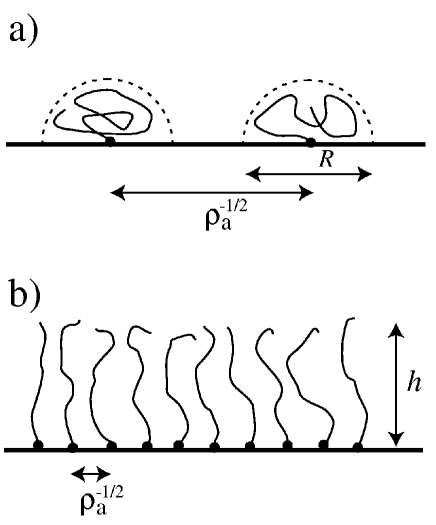
Figure 1: For grafted chains, one distinguishes between: a) the mushroom regime, where the distance between chains, $\rho_{a}^{-1/2}$, is larger than the size $R$ of a polymer coil; and, b) the brush regime, where the distance between chains is smaller than the unperturbed coil size. Here, the chains are stretched away from the surface due to repulsive interactions between monomers. The brush height $h$ scales linearly with the polymerization index, $h\sim N$, and thus is larger than the unperturbed coil radius $R$ which in the good-solvent regime scales according to Flory as $R_{F}\sim aN^{\nu}$.

The characteristic parameter for brush systems is the anchoring or grafting density $\rho_{a}$, which is the inverse of the average area available for each polymer at the surface. For small grafting densities, $\rho_{a}<\rho_{a}^{*}$, the polymer chains will be far apart from each other and hardly interact, as schematically shown in Fig.1a. The polymers in this case form well separated mushrooms at the surface. The grafting density at which chains just start to overlap is determined by $\rho_{a}^{*}\sim R^{-2}$ where $R$ is the typical radius or size of a chain. In good solvent conditions (that is for swollen chains), the chain radius follows the Flory prediction $R_{F}\sim aN^{3/5}$ where $N$ is the polymerization index or monomer number of the chain, and $a$ is a characteristic microscopic length scale of the polymer that incorporates monomer size as well as backbone stiffness. The crossover grafting density for a polymer under good-solvent conditions follows as $\rho_{a}^{*}\sim a^{-2}N^{-6/5}$. For large grafting densities, $\rho>\rho^{*}$, the chains are strongly overlapping. This situation is depicted in Fig.1b. Since we assume the solvent to be good, monomers repel each other. The lateral separation between the polymer coils is fixed by the grafting density, so that the polymers extend away from the grafting surface in order to avoid each other. The resulting structure is called a polymer brush, with a vertical height $h$ which greatly exceeds the unperturbed coil radius $R$ [20, 21, 22]. Similar stretched structures occur in many other situations, such as diblock copolymer melts in the strong segregation regime [23, 6], or star polymers under good solvent conditions[24]. Theory is mostly concerned with predicting the layer height $h$, but also the detailed monomer density profile and resulting forces of lateral or vertical brush compression as a function of the various system parameters.

The understanding of grafted polymer systems progressed substantially with the advent of experimental techniques such as: surface-force-balance[8], small-angle-neutron scattering[9], neutron[11, 25] and X-ray[26] diffraction, and ellipsometry[14]. Of equal merit was the advancement in the theoretical methodology ranging from field theoretical methods and scaling arguments to numerical simulations, which will be amply reviewed in this chapter.

2 Polymer basics

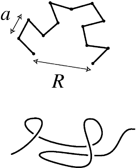
Figure 2: Top: Freely-jointed chain (FJC) model, where $N$ bonds of length $a$ are connected to form a flexible chain with a certain end-to-end distance $R$. Bottom: In the simplified model, appropriate for more advanced theoretical calculations, a continuous line is governed by some bending rigidity or line tension. This continuous model can be used when the relevant length scales are much larger than the monomer size.

The main parameters used to describe a polymer chain are the polymerization index $N$, which counts the number of repeat units or monomers along the chain, and the size of one monomer or the distance between two neighboring monomers. The monomer size ranges from a few Angstroms for synthetic polymers to a few nanometers for biopolymers. The simplest theoretical description of flexible chain conformations is achieved with the so-called freely-jointed chain (FJC) model, where a polymer consisting of $N+1$ monomers is represented by $N$ bonds defined by bond vectors ${\bf r}_{j}$ with $j=1,\ldots N$. Each bond vector has a fixed length $|{\bf r}_{j}|=a$ corresponding to the Kuhn length, but otherwise is allowed to rotate freely and independently of its neighbors, as is schematically shown in Fig.2 (top). This model of course only gives a coarse-grained description of real polymer chains, but we will later see that by a careful interpretation of the Kuhn length $a$ and the monomer number $N$, an accurate description of the large-scale properties of real polymer chains is possible. The main advantage is that due to the simplicity of the FJC model, many interesting observables (such as chain size or distribution functions) can be calculated with relative ease. We demonstrate this by calculating the mean end-to-end radius of such a FJC polymer. Fixing one of the chain ends at the origin, the position of the $(k+1)$-th monomer is given by the vectorial sum

$${\bf R}_{k}=\sum_{j=1}^{k}{\bf r}_{j}~{}.$$ (1)

Because two arbitrary bond vectors are uncorrelated in this simple model, the thermal average over the scalar product of two different bond vectors vanishes, $\langle{\bf r}_{j}\cdot{\bf r}_{k}\rangle=0$ for $j\neq k$, while the mean squared bond vector length is simply given by $\langle{\bf r}_{j}^{2}\rangle=a^{2}$. It follows that the mean squared end-to-end radius $R_{N}^{2}$ is proportional to the number of monomers,

$$R_{0}^{2}\equiv\langle{\bf R}_{N}^{2}\rangle=Na^{2}=La,$$ (2)

where the contour length of the chain is given by $L=Na$. $R_{0}$ denotes the mean end-to-end radius of an ideal chain, and according to Eq.(2), it scales as $R_{0}=aN^{1/2}$. Experimentally one often knows, via knowledge of the chemical structure and polymer mass, the length $L$ and, via light-scattering, the radius $R$ of a chain. Using the above scaling results, valid for a non-interacting chain, the Kuhn length follows as $a=R_{0}^{2}/L$ and the effective monomer number as $N=L/a$, which allows treatment of real chains with a complicated local conformational structure within the FJC model. Note that the so-determined Kuhn length $a$ is usually larger than the actual monomer-size, since it takes back-bone stiffness effects into account. Likewise, the determined effective monomer number $N$ is typically smaller than the actual (chemical) number of monomers in the chain.

In many theoretical calculations aimed at elucidating large-scale properties, the simplification is carried even a step further and a continuous model is used, as schematically shown in Fig.2 (bottom). In such models the polymer backbone is replaced by a continuous line and all microscopic details are neglected. The chain is then only characterized by its length $L$ and radius $R$.

2.1 Polymer swelling and collapse

The models discussed so far describe ideal chains and do not account for interactions between monomers which typically consist of some short-ranged repulsion and long-ranged attraction. Including these interactions will give a different scaling behavior for long polymer chains. The end-to-end radius, $R=\sqrt{\langle R^{2}_{N}\rangle}$, can be written for $N\gg 1$ as

$$R\simeq aN^{\nu}$$ (3)

which defines the so-called swelling exponent $\nu$. As we have seen, for an ideal polymer chain (no interactions between monomers), Eq.(2) implies $\nu=1/2$. This situation is realized for experimental polymers at a certain temperature or solvent conditions when the attraction between monomers exactly cancels the steric repulsion (which is due to the fact that the monomers cannot penetrate each other). This situation can be achieved in the condition of theta solvents. In good solvents, on the other hand, the monomer-solvent interaction is more attractive than the monomer-monomer interaction, in other words, the monomers try to avoid each other in solution. As a consequence, single polymer chains in good solvents have swollen spatial configurations dominated by the steric repulsion, characterized by an exponent $\nu\simeq 3/5$, leading to the Flory radius $R_{F}\sim aN^{3/5}$. This spatial size of a polymer coil is much smaller than the extended contour length $L=aN$ but larger than the size of an ideal chain $R_{0}=aN^{1/2}$, i.e. $R_{0}\ll R_{F}\ll L$ in the limit $N\rightarrow\infty$. The reason for this behavior is conformational entropy (which prevents full stretching of the chain) combined with the favorable interaction between monomers and solvent molecules in good solvents (which leads to a more open structure than an ideal chain). In the opposite case of bad or poor solvent conditions, the effective interaction between monomers is attractive, leading to collapse of the chains and to their precipitation from solution. In this case, the polymer volume, like any space filling object embedded in three-dimensional space, scales proportional to its weight as $R^{3}\sim N$, yielding an exponent $\nu=1/3$.

The standard way of taking into account interactions between monomers is the Flory theory, which treats these interactions on an approximate mean-field level[1, 2, 3]. Let us first consider the case of repulsive interactions between monomers, which can be described by a positive second-virial coefficient $v_{2}$ and corresponds to the good-solvent condition. For pure hard-core interactions and with no additional attractions between monomers, the second virial coefficient (which corresponds to the excluded volume) is of the order of the monomer volume, i.e. $v_{2}\sim a^{3}$. The repulsive interaction between monomers, which tends to swell the chain, is counteracted and balanced by the ideal chain elasticity, which is brought about by the entropy loss associated with stretching the chain. The origin is that the number of polymer configurations having an end-to-end radius of the order of the unperturbed end-to-end radius is large. These configurations are entropically favored over configurations characterized by a large end-to-end radius, for which the number of possible polymer conformations is drastically reduced. The standard Flory theory for a flexible chain of radius $R$ is based on writing the free energy $F$ of a chain (in units of the thermal energy $k_{B}T$) as a sum of two terms (omitting numerical prefactors)

$$F\simeq\frac{R^{2}}{R_{0}^{2}}+v_{2}R^{3}\left(\frac{N}{R^{3}}\right)^{2}~{},$$ (4)

where the first term is the entropic elastic energy associated with swelling a polymer chain to a radius $R$, proportional to the effective spring constant of an ideal chain, $k_{B}T/R_{0}^{2}$, and the second term is the second-virial repulsive energy proportional to the coefficient $v_{2}$, and the segment density squared. It is integrated over the volume $R^{3}$. The optimal radius $R$ is calculated by minimizing this free energy and gives the swollen radius

$$R_{F}\sim a(v_{2}/a^{3})^{1/5}N^{\nu}~{},$$ (5)

with $\nu=3/5$. For purely steric interactions with $v_{2}\simeq a^{3}$ we obtain $R\sim aN^{\nu}$. For weakly interacting monomers, $0<v_{2}<a^{3}$, one finds that the swollen radius Eq.(5) is only realized above a minimal monomer number $N\simeq(v_{2}/a^{3})^{-2}$ below which the chain statistics is unperturbed by the interaction and the scaling of the chain radius is Gaussian and given by Eq.(2).

In the opposite limit of a negative second virial coefficient, $v_{2}<0$, corresponding to the bad or poor solvent regime, the polymer coil will be collapsed due to attraction between monomers. In this case, the attraction term in the free energy is balanced by the third-virial term in a low-density expansion (where we assume that $v_{3}>0$),

$$F\simeq v_{2}R^{3}\left(\frac{N}{R^{3}}\right)^{2}+v_{3}R^{3}\left(\frac{N}{R^{3}}\right)^{3}~{}.$$ (6)

Minimizing this free energy with respect to the chain radius one obtains

$$R\simeq(v_{3}/|v_{2}|)^{1/3}N^{\nu}$$ (7)

with $\nu=1/3$. This indicates the formation of a compact globule, since the monomer density inside the globule, $\rho\sim N/R^{3}$, is independent of the chain length. The minimal chain length to observe a collapse behavior is $N\sim(v_{3}/a^{3}v_{2})^{2}$. For not too long chains and a second virial coefficient not too much differing from zero, the interaction is irrelevant and one obtains effective Gaussian or ideal behavior. It should be noted, however, that even small deviations from the exact theta conditions (defined by strictly $v_{2}=0$) will lead to chain collapse or swelling for very long chains.

2.2 Charged polymers

A polyelectrolyte (PE) is a polymer with a fraction $f$ of charged monomers. When this fraction is small, $f\ll 1$, the PE is weakly charged, whereas when $f$ is close to unity, the polyelectrolyte is strongly charged. There are two common ways to control $f$ [17]. One way is to polymerize a heteropolymer mixing strongly acidic and neutral monomers as building blocks. Upon contact with water, the acidic groups dissociate into positively charged protons (H⁺) that bind immediately to water molecules, and negatively charged monomers. Although this process effectively charges the polymer molecules, the counter-ions make the PE solution electro-neutral on larger length scales. The charge distribution along the chain is quenched during the polymerization stage, and it is characterized by the fraction of charged monomers on the chain, $f$. In the second way, the PE is a weak polyacid or polybase. The effective charge of each monomer is controlled by the $pH$ and the salt concentration of the solution[27]. Moreover, this annealed fraction depends on the local electric potential which is in particular important for adsorption or binding processes since the local electric potential close to a strongly charged surface or a second charged polymer can be very different from its value in the bulk solution and therefore modify the polyelectrolyte charge[28].

Counterions are attracted to the charged polymers via long-ranged Coulomb interactions; this physical association typically leads to a rather loosely bound counter-ion cloud around the PE chain. Because of this background of a polarizable and diffusive counterion cloud, there is a strong influence of the counterion distribution on the PE structure and vice versa. Counterions contribute significantly towards bulk properties, such as the osmotic pressure, and their translational entropy is responsible for the generally good water solubility of charged polymers. In addition, the statistics of PE chain conformations is governed by intra-chain Coulombic repulsion between charged monomers; this results in a more extended and swollen conformation of PE’s as compared to neutral polymers and gives rise to the characteristically high viscosity of polyelectrolyte solutions (hence their use as viscosifiers in food industry).

For polyelectrolytes, electrostatic interactions provide the driving force for their salient features and have to be included in any theoretical description. The reduced electrostatic interaction between two point-like charges can be written as $q_{1}q_{2}v(r)$ where

$$v(r)=\ell_{B}/r$$ (8)

is the Coulomb interaction between two elementary charges in units of $k_{B}T$ and $q_{1}$ and $q_{2}$ are the valencies (or the reduced charges in units of the elementary charge $e$). The Bjerrum length $\ell_{B}$ is defined as

$$\ell_{B}=\frac{e^{2}}{4\pi\varepsilon k_{B}T},$$ (9)

where $\varepsilon$ is the medium dielectric constant. It denotes the distance at which the Coulombic interaction between two unit charges in a dielectric medium is equal to thermal energy ($k_{B}T$). It is a measure of the distance below which the Coulomb energy is strong enough to compete with the thermal fluctuations; in water at room temperatures, one finds $\ell_{B}\approx 0.7$ nm.

In biological systems and most industrial applications, the aqueous solution contains in addition to the counterions mobile salt ions. Salt ions of opposite charge are drawn to the charged object and modify the counterion cloud around it. They effectively reduce or screen the charge of the object. The effective (screened) electrostatic interaction between two charges $q_{1}$ and $q_{2}$ in the presence of salt ions and a polarizable solvent can be written as $q_{1}q_{2}v_{\rm DH}(r)$, with the Debye-Hückel (DH) potential $v_{\rm DH}(r)$ given (in units of $k_{B}T$) by

$$v_{\rm DH}(r)=\frac{\ell_{B}}{r}{\rm e}^{-\kappa r}~{}.$$ (10)

The exponential decay is characterized by the screening length $\kappa^{-1}$, which is related to the salt concentration $c_{\rm salt}$ by $\kappa^{2}=8\pi q^{2}\ell_{B}c_{\rm salt}~{}$, where $q$ denotes the valency of $q:q$ salt. At physiological conditions the salt concentration is $c_{\rm salt}\approx 0.1$ M and for monovalent ions ($q=1$) this leads to $\kappa^{-1}\approx 1$ nm. This means that although the Coulombic interactions are long-ranged, in physiological conditions they are highly screened above length scales of a few nanometers, which results from multi-body correlations between ions in a salt solution.

For charged polymers, the effective bending stiffness and thus the Kuhn length is increased due to electrostatic repulsion between monomers[29, 30, 31, 32, 33, 34, 35]. This effect modifies considerably not only the PE behavior in solution but also their adsorption characteristics[36].

A peculiar phenomenon occurs for highly charged PE’s and is known as the Manning condensation of counter-ions [37, 38, 39]. This phenomenon constitutes a true phase transition in the absence of added salt ions. For a single rigid PE chain represented by an infinitely long and straight cylinder with a linear charge density $\tau$ larger than the threshold

$$\ell_{B}\tau q=1~{},$$ (11)

where $q$ is the counter-ion valency, it was shown that counter-ions condense on the oppositely charged cylinder even in the limit of infinite system size. For a solution of stiff charged polymers this corresponds to the limit where the inter-chain distance tends to infinity. This effect is not captured by the linear Debye-Hückel theory. A simple heuristic way to incorporate the non-linear Manning condensation is to replace the bare linear charge density $\tau$ by the renormalized one, $\tau_{\rm renorm}=1/(q\ell_{B})$, whenever $\ell_{B}\tau q>1$ holds. This procedure, however, is not totally satisfactory at high salt concentrations [40, 41]. Also, real polymers have a finite length, and are neither completely straight nor in the infinite dilution limit [42]. Still, Manning condensation has an experimental significance for polymer solutions[43] because thermodynamic quantities, such as counter-ion activities [44] and osmotic coefficients [45], show a pronounced signature of Manning condensation. Locally, polymer segments can be considered as straight over length scales comparable to the persistence length. The Manning condition Eq. (11) usually denotes a region where the binding of counter-ions to charged chain sections begins to deplete the solution from free counter-ions.

3 Neutral grafted polymers

3.1 Scaling approach

The scaling behavior of the brush height $h$ can be analyzed using a Flory-like mean–field theory, which is a simplified version of the original Alexander theory [21] for polymer brushes. The stretching of the chain leads to an entropic free energy loss of $h^{2}/R_{0}^{2}$ per chain, and the repulsive energy density due to unfavorable monomer-monomer contacts is proportional to the squared monomer density times the excluded-volume parameter $v_{2}$. The derivation is thus analogous to the calculation of the Flory radius of a chain in good solvent shown in Section 2.1, except that now the grafting density $\rho_{a}$ plays a decisive role and controls the amount of stretching of the chains. The free energy per chain (and in units of $k_{B}T$) is then

$$F\simeq\frac{h^{2}}{a^{2}N}+v_{2}\left(\frac{\rho_{a}N}{h}\right)^{2}\frac{h}{\rho_{a}}~{}.$$ (12)

The equilibrium height is obtained by minimizing Eq. (12) with respect to $h$, and the result is

$$h_{0}=N\left(2v_{2}a^{2}\rho_{a}/3\right)^{1/3}~{}$$ (13)

where the numerical constants have been added for numerical convenience in the following considerations. The vertical size of the brush scales linearly with the polymerization index $N$, a clear signature of the strong stretching of the polymer chains, as was originally obtained by Alexander [21]. At the overlap threshold, $\rho_{a}^{*}\sim a^{-2}N^{-6/5}$, the height scales as $h_{0}\sim N^{3/5}$, and thus agrees with the scaling of an unperturbed chain radius in a good solvent, Eq.(5), as it should. The simple scaling calculation predicts the brush height $h$ correctly in the asymptotic limit of long chains and strong overlap. It has been confirmed by experiments [9, 8, 11] and computer simulations [46, 47].

3.2 Mean-field calculation

The above scaling result assumes that all chains are stretched to exactly the same height, leading to a step-like shape of the density profile. Monte-Carlo and numerical mean–field calculations confirm the general scaling of the brush height, but exhibit a more rounded monomer density profile which goes continuously to zero at the outer perimeter [46]. A big step towards a better understanding of stretched polymer systems was made by Semenov [23], who recognized the importance of classical paths for such systems.

The classical polymer path is defined as the path which minimizes the free energy, for given start and end positions, and thus corresponds to the most likely path a polymer can take. The name follows from the analogy with quantum mechanics, where the classical motion of a particle is given by the quantum path with maximal probability. Since for strongly stretched polymers the fluctuations around the classical path are weak, it is expected that a theory that takes into account only classical paths, is a good approximation in the strong-stretching limit. To quantify the stretching of the brush, let us introduce the (dimensionless) interaction parameter $\beta$, defined as

$$\beta\equiv N\left(\frac{3v_{2}^{2}\rho_{a}^{2}}{2a^{2}}\right)^{1/3}=\frac{3}{2}\left(\frac{h_{0}}{aN^{1/2}}\right)^{2}~{},$$ (14)

where $h_{0}$ is the brush height according to Alexander’s theory, compare Eq. (13). The parameter $\beta$ is proportional to the square of the ratio of the Alexander prediction for the brush height, $h_{0}$, and the unperturbed Gaussian chain radius $R_{0}\sim aN^{1/2}$, and, therefore, is a measure of the stretching of the brush based on the scaling prediction. We will later see that the actual stretching of the brush is not correctly described by the scaling result for short or weakly interacting chains. Constructing a classical theory in the infinite-stretching limit, defined as the limit $\beta\rightarrow\infty$, it was shown independently by Milner et al. [48] and Skvortsov et al. [49] that the resulting monomer density profile $\rho(z)$ depends only on the vertical distance $z$ from the grafting surface and has in fact a parabolic profile. Normalized to unity, the density profile is given by[48, 49]

$$\frac{\rho(z)h_{0}}{\rho_{a}N}=\left(\frac{3\pi}{4}\right)^{2/3}-\left(\frac{\pi z}{2h_{0}}\right)^{2}~{}.$$ (15)

The brush height, i.e., the value of $z$ for which the monomer density becomes zero, is given by $z^{*}=(6/\pi^{2})^{1/3}h_{0}$ and is thus proportional to the scaling prediction for the brush height, Eq.(13). The parabolic brush profile has subsequently been confirmed in computer simulations [46, 47] and experiments [9] as the limiting density profile in the strong-stretching limit, and constitutes one of the cornerstones in this field. Intimately connected with the density profile is the distribution of polymer end points, which is non-zero everywhere inside the brush (as we will demonstrate later on), in contrast with the original scaling description leading to Eq. (13).

However, deviations from the parabolic profile become progressively important as the length of the polymers $N$ or the grafting density $\rho_{a}$ decreases. In a systematic derivation of the mean–field theory for Gaussian brushes [50] it was shown that the mean–field theory is characterized by a single parameter, namely the stretching parameter $\beta$. In the limit $\beta\rightarrow\infty$, the difference between the classical approximation and the mean–field theory vanishes, and one obtains the parabolic density profile. For finite $\beta$ the full mean–field theory and the classical approximation lead to different results and both show deviations from the parabolic profile.

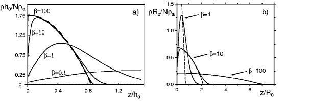
Figure 3: Self-consistent mean-field results for the density profile (normalized to unity) of a brush for different values of the interaction parameter $\beta$. In a) the distance from the grafting surface is rescaled by the scaling prediction for the brush height, $h_{0}$, and in b) it is rescaled by the unperturbed polymer radius $R_{0}$. As $\beta$ increases, the density profiles approach the parabolic profile (shown as dashed lines).

In Fig.3 we show the density profiles (normalized to unity) for four different values of $\beta$, obtained with the full mean–field theory [50]. In a) the distance from the grafting surface is rescaled by the scaling prediction for the brush height, $h_{0}$, and in b) it is rescaled by the unperturbed polymer radius $R_{0}$. For comparison, we also show the asymptotic result according to Eq. (15) as dashed lines. The self-consistent mean–field equations are solved in the continuum limit, where the results depend only on the single parameter $\beta$ and direct comparison with other continuum theories becomes possible. As $\beta$ increases, the density profiles approach the parabolic profile and already for $\beta=100$ the density profile obtained within mean–field theory is almost indistinguishable from the parabolic profile denoted by a thick dashed line in Fig. 3a. What is interesting to see is that for small values of the interaction parameter $\beta$, the numerically determined density profiles exhibit a larger brush height than the asymptotic prediction. This has to do with the fact that entropic effects, due to steric polymer repulsion from the grafting surface, are not accounted for in the infinite-stretching approximation. Experimentally, the achievable $\beta$ values are below $\beta\simeq 50$, which means that deviations from the asymptotic parabolic profile are important. For moderately large values of $\beta>10$, the classical approximation (not shown here), derived from the mean–field theory by taking into account only one polymer path per end-point position, is still a good approximation, as judged by comparing density profiles obtained from both theories [50], except very close to the surface. Unlike mean-field theory, the classical theory misses completely the depletion effects at the substrate. Depletion effects at the substrate lead to a pronounced density depression close to the grafting surface, as is clearly visible in Fig. 3.

Let us now turn to the thermodynamic behavior of a polymer brush. Using the Alexander scaling model, we can calculate the free energy per chain by putting the result for the optimal brush height, Eq. (13), into the free-energy expression, Eq. (12), and obtain

$$F\sim\beta\sim N\left(v_{2}\rho_{a}/a\right)^{2/3}.$$ (16)

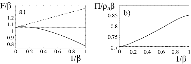
Figure 4: a) Mean-field result (solid line) for the rescaled brush free energy per polymer as a function of the inverse interaction parameter $1/\beta$. The infinite stretching result is indicated by a horizontal dotted line, the broken straight line denotes the infinite stretching result with the leading correction due to the finite end-point distribution entropy. b) Rescaled lateral pressure within mean-field theory (solid line) compared with the asymptotic infinite-stretching result (dotted line).

In Figure 4a we show the rescaled free energy per chain within the full mean-field framework (solid line) in comparison with the infinite stretching result (dotted horizontal line) and including the leading correction due to the finite entropy of the end-point distribution (broken line)[50]. In the infinite-stretching limit, i.e. for $1/\beta\rightarrow 0$, all curves converge. The free energy is not directly measurable, but the lateral pressure can be determined using the Langmuir film balance technique. The osmotic surface pressure $\Pi$ is related to $F$, the free energy per chain, by

$$\Pi=-\frac{\partial(F\rho_{a}A)}{\partial A}=\rho_{a}^{2}\frac{\partial F}{\partial\rho_{a}}=\frac{2\rho_{a}}{3}\left(F-\frac{\partial F/\beta}{\partial\beta^{-1}}\right)$$ (17)

In Figure 4b we show the rescaled osmotic pressure obtained within the mean-field approach (solid line). In the infinite-stretching limit, one expects a scaling as $\Pi\sim\rho_{a}^{5/3}$ which is shown as a dotted line. One notes that the more accurate mean-field result gives a pressure which is strictly larger than the asymptotic infinite stretching result, in agreement with previous calculations and experiments[51, 12, 52, 53, 54]. In the presence of excluded-volume correlations, i.e., when the chain overlap is rather moderate, the scaling of the brush height $h$, Eq.(13), is still correctly predicted by the Alexander calculation, but the prediction for the free energy, Eq.(16), is in error. Including correlations [21], the free energy is predicted to scale as $F\sim N\rho_{a}^{5/6}$. leading to a pressure which scales as $\Pi\sim\rho_{a}^{11/6}$ in the presence of correlations. However, all these theoretical predictions do not compare well with experimental results for the surface pressure of a compressed brush [12] which has to do with the fact that experimentally, chains are rather short so that one essentially is dealing with a crossover situation between the mushroom and brush regimes. An alternative theoretical method to study tethered chains is the so-called single-chain mean–field method [51], where the statistical mechanics of a single chain is treated exactly, and the interactions with the other chains are taken into account on a mean-field level. This method is especially useful for short chains, where fluctuation effects are important, and for dense systems, where excluded volume interactions play a role. The calculated profiles and brush heights agree very well with experiments and computer simulations. Moreover, these calculations explain the pressure isotherms measured experimentally [12] and in molecular-dynamics simulations [55].

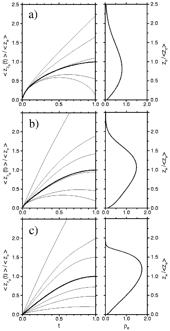
Figure 5: Left: Mean-field results for the rescaled averaged polymer paths which end at a certain distance $z_{e}$ from the wall for $\beta=\,\,$1, 10, 100 (from top to bottom), corresponding to stretching values of $\gamma=1.1,1.9,5.6$. The thick solid line shows the unconstrained mean path obtained by averaging over all end-point positions. Note that the end-point stretching is small but finite for all finite stretching parameters $\beta$. Right: End-point distributions.

A further interesting question concerns the behavior of individual polymer paths. As was already discussed for the infinite-stretching theories ($\beta\rightarrow\infty$), polymers paths do end at any distance from the surface. In the left part of Figure 5 we show mean-field results for the rescaled averaged polymer paths which end at a certain distance $z_{e}$ from the wall for $\beta=\,\,$1, 10, 100 (from top to bottom). Analyzing the polymer paths which end at a common distance from the surface, two rather unexpected features are obtained: i) free polymer ends, in general, are stretched; and, ii) the end-points lying close to the substrate are pointing towards the surface (such that the polymer path first turns away from the grafting surface before moving back towards it). In contrast, end-points lying beyond a certain distance from the substrate, point away from the surface (such that the paths move monotonously towards the surface). As we will explain shortly below, these two features have been confirmed in molecular-dynamics simulations [56]. They are not an artifact of the continuous self-consistent theory used in Ref. [50] nor are they due to the neglect of fluctuations. These are interesting results, especially since it has been long assumed that free polymer ends are unstretched, based on the assumption that no forces act on free polymer ends. The thick solid line shows the unconstrained mean path obtained by averaging over all end-point positions. Note that the end-point stretching is small but finite for all finite stretching parameters $\beta$. The right panel exhibits the end-point distributions, which, obviously, are finite over the whole range of vertical heights.

3.3 Molecular Dynamics simulations

We now present results from Molecular Dynamics simulations in which all the chain monomers are coupled to a heat bath. The chains interact via the repulsive portion of a shifted Lennard-Jones potential with a Lennard-Jones diameter $\sigma$, which corresponds to a good solvent situation. For the bond potential between adjacent polymer segments we take a FENE (nonlinear bond) potential which gives an average nearest-neighbor monomer-monomer separation of typically $a\approx 0.97\sigma$. In the simulation box with a volume $L\times L\times L_{z}$ there are 50 (if not stated otherwise) chains each of which consists of $N+1$ monomers with varying monomer number $N=20,\,30,\,50$, as indicated. The box length $L$ in $x-$ and $y-$direction was chosen to give anchoring densities $\rho_{a}$ from 0.02$\,\sigma^{-2}$ to 0.17$\,\sigma^{-2}$. The first monomer of each chain is firmly and randomly attached to the grafting surface at $z=0$. The mean square end-to-end distance of identical free (i.e. unanchored) chains was for the case $N=50$ found to be $R_{F}\equiv\langle({\bf r}_{N}-{\bf r}_{0})^{2}\rangle_{\rm free}^{1/2}=12.55\sigma$. For more details consult [56].

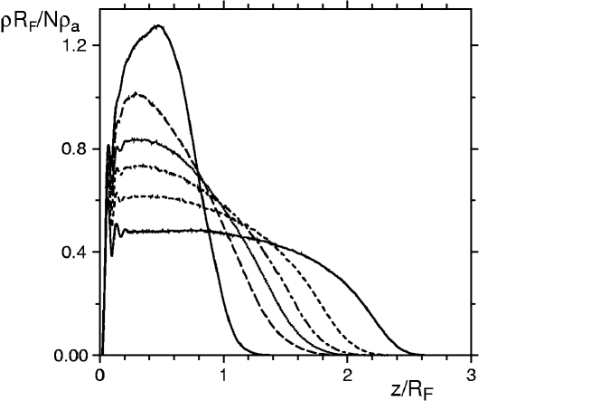
Figure 6: Simulation results for the normalized monomer number density, $\rho(z)R_{F}/N\rho_{a}$, as a function of the scaled distance from the grafting surface $z/R_{F}$ for anchored chains of length $\,N=50\,$ and grafting densities $\,\rho_{a}\sigma^{2}$ = 0.02, 0.04, 0.06, 0.09, and 0.17 (from top to bottom). Note that $R_{F}$ is determined within the simulation for a single, free polymer chain.

Figure 6 shows the behavior of the reduced monomer density $\rho(z)R_{F}/N\rho_{a}\,$ at increasing anchoring density. The stretching of the chains with increasing surface coverage, which is due to the repulsion between monomers, is evident. This plot has to be compared with Figure 3b, where the same type of rescaling has been used. However, note that at this point, direct and quantitative comparison is not possible, since it is a priori not clear which value of the interaction parameter $\beta$ in the self-consistent calculation corresponds to which set of simulation parameters $\sigma$, $N$, $\rho_{a}$.

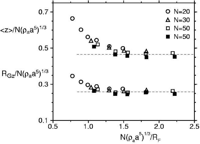
Figure 7: Simulation results for the rescaled average monomer height $h/(N\rho_{a}^{1/3}a^{5/3})$ (top) and the vertical component of the radius of gyration $R_{Gz}/(N\rho_{a}^{1/3}a^{5/3})$ (bottom) versus the scaling variable $N(\rho_{a}a^{5})^{1/3}/R_{F}$ for different chains lengths as indicated in the figure. The open/filled symbols correspond to extensible and non-extensible chains, respectively, which is controlled within the simulation by the strength of the FENE bond potentials. As one can see, for large values of the parameter combination $N(\rho_{a}a^{5})^{1/3}/R_{F}$ the data saturate at a plateau and are thus in agreement with the scaling prediction.

The theoretically predicted scaling law of the brush height $h_{0}\sim N\rho_{a}^{1/3}$ has been confirmed in several simulations[47]. Provided $\rho_{a}$ is above the critical overlap density $\rho_{a}^{*}\sim N^{-6/5}$, the brush height, as measured by the first moment of the monomer density distribution $\langle z\rangle=\int\!z\rho(z)dz/\!\int\!\rho(z)dz$, should approach the predicted scaling form. Figure 7 shows this behavior in an appropriate scaling plot of the average brush height $\langle z\rangle$ and the $z$-component of the radius of gyration $R_{G}\equiv\langle\,\sum_{i=0}^{N}({\bf r}_{i}-{\bf r}_{cm})^{2}/(N+1)\rangle^{1/2}$ where ${\bf r}_{cm}$ is the position of the center of mass. For the scaling plot the brush height and radius of gyration are divided by the scaling prediction $h_{0}\sim N\rho_{a}^{1/3}a^{5/3}$ and plotted as a function of the analogue of the interaction parameter, namely $h_{0}/R_{F}\sim N\rho_{a}^{1/3}a^{5/3}/R_{F}$, where $a$ and $R_{F}$ are determined from the simulation in the absence of a grafting wall. In this way we obtain an universal crossover point $N\rho_{a}^{1/3}a^{5/3}/R_{F}\approx 1.4$. Thus, for the chain length $N$=50, the case we discussed most, one can be sure to reach the asymptotic scaling regime for the larger grafting densities.

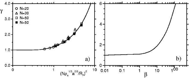
Figure 8: Effective stretching factor $\,\gamma=\langle z_{e}(\rho_{a})/z_{e}(0)\rangle$ as obtained a) within the simulation as a function of the scaled anchoring density $(N\rho_{a}^{1/3}a^{5/3}/R_{F})^{2}$ and b) from the self-consistent field theory as a function of the interaction parameter $\beta$. The comparison between the simulation results and the analytical results allows to determine the effective $\beta$ parameter of a particular simulation set.

A general problem when comparing experimental, simulation and analytical results among each other is that the different parameters have to be matched in a meaningful way. One such way is based on the relative stretching of chains in a brush. In Figure 8 we plot in a) simulation results for the stretching ratio

$$\gamma=\,\langle z_{e}({\rho_{a}})\rangle/\langle z_{e}({\rho_{a}}=0)\rangle$$ (18)

which is the averaged end-point height for a finite grafting density divided by the end-point height for vanishing grafting density. The stretching ratio is plotted as a function of the scaled anchoring density $(N\rho_{a}^{1/3}a^{5/3}/R_{F})^{2}$ which is the analogue of the interaction parameter $\beta$. It is seen that the different chain lengths and grafting densities scale quite nicely. Clearly, for short chains or low grafting densities, that is in the mushroom regime, the stretching ratio $\gamma$ approaches unity. The highest stretching ratio reached in the simulations is $\gamma\approx 2.7$. In Figure 8b we show mean-field results for the stretching ratio $\gamma$ as a function of the interaction parameter $\beta$. The general shape of the curve is similar. Matching the stretching ratios of the simulation and the mean-field calculation allows to determine the effective $\beta$ value corresponding to a particular simulation run. As an example, for the most highly stretched simulation with $\gamma\approx 2.7$, we estimate an effective interaction parameter of $\beta\approx 25$. A similar matching procedure is possible with experimental data.

In agreement with the mean-field profiles shown in Figure 3, the monomer density obtained from the simulations in Figure 6 decays smoothly to zero at distances far from the anchoring plane. However, comparing the shape of the profiles in more detail, one notes a region over which the simulation profiles become rather flat for anchoring densities $\rho_{a}>0.1\sigma^{-2}$, in contrast to the mean-field results. According to Figure 8, this corresponds to stretching factors $\gamma>2$ or $\beta>10$. This discrepancy can be traced back to the neglect of higher-order virial terms in the analytical theory, which beome important at elevated monomer densities.

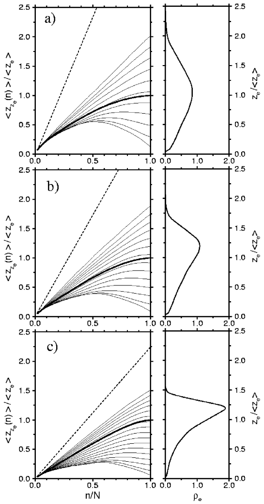
Figure 9: Left: Simulation results for the rescaled averaged polymer paths which end at a certain distance $z_{e}$ from the wall for $\rho_{a}\sigma^{2}=\,\,$0.02, 0.06, 0.17 (from top to bottom), corresponding to stretching values of $\gamma=1.3,1.8,2.7$. The thick solid line shows the unconstrained mean path obtained by averaging over all end-point positions. Right: End-point distributions. All data are obtained for simulations with 50 chains consisting of $N=50$ monomers each.

We also looked at individual polymer paths within the simulation. The scaled average polymer paths with a given fixed end-point distance $\,z_{e}$, $\langle z_{z_{e}}(n)\rangle/\langle z_{e}\rangle$, are shown in Figure 9 for three typical anchoring densities corresponding to stretching factors $\gamma\approx\,\,$1.3, 1.8, and 2.7, from top to bottom. To get an idea of their relative weight we plot the polymer paths together with the normalized density of free ends $\,\rho_{e}(z)\,$ (shown in the right panel). The trajectories are very similar to those predicted by the mean-field theory (see Figure 5). Paths which end far from the anchoring surface are stretched through their entire length, including the free end point. The paths which end at the outer rim of the distribution are almost uniformly stretched and appear almost as a straight line. On the other hand, paths which end close to the anchoring surface are non-monotonic, first moving away from the wall, reaching a maximal distance, and then turning back towards the anchoring surface. Except at the maximum, all paths are stretched everywhere, including the end point. The straight broken lines are added for comparison and denote the maximally stretched possible path, which consists of a fully oriented and straight polymer. As can be seen from Figure 5 as well as from Figure 9, the end-point stretching, proportional to $(dz/ds)$ or $(dz/dn)$, respectively, is positive for some particular paths and negative for others, so that the average, plotted as thick line in the Figures, is typically quite small. This reconciles the present results with the infinite-stretching results by Milner, Witten and Cates [48] and Zhulina and co-workers [49], where the chains were assumed to be unstretched at their ends regardless of their end-point position: this assumption turns out to be acceptable on average if the stretching of the chains is large, i.e., for large $\beta$.

3.4 Additional effects

As we described earlier, the main interest in end-adsorbed or grafted polymer layers stems from their ability to stabilize surfaces against van-der-Waals attraction. The force between colloids with grafted polymers is repulsive if the polymers do not adsorb on the grafting substrates [57], that is, in the absence of polymer bridges and loops. A stringent test of brush theories was possible with accurate experimental measurements of the repulsive interaction between two opposing grafted polymer layers using a surface force apparatus [8]. The resultant force could be fitted very nicely by the infinite-stretching theory of Milner et al. [58]. It was also shown that polydispersity effects, as appear in experiments, have to be taken into account theoretically in order to obtain a good fit of the data [59].

So far we assumed that the polymer grafted layer is in contact with a good solvent. In this case, the grafted polymers try to minimize their mutual contacts by stretching out into the solvent. If the solvent is bad, the monomers try to avoid the solvent by forming a collapsed brush, the height of which is considerably reduced with respect to the good-solvent case. It turns out that the collapse transition, which leads to phase separation in the bulk, is smeared out for the grafted layer and does not correspond to a true phase transition [60]. The height of the collapsed layer scales linearly in $\rho_{a}N$, which reflects the constant density within the brush, in agreement with experiments [61]. Some interesting effects have been described theoretically [62] and experimentally [61] for brushes in mixtures of good and bad solvent, which can be rationalized in terms of a partial solvent demixing.

For a theta solvent ($v_{2}=0$) the relevant interaction is described by the third-virial coefficient; using a simple Alexander approach similar to the one leading to Eq. (13), the brush height is predicted to vary with the grafting density as $h\sim\rho_{a}^{1/2}$, in agreement with computer simulations [63].

Up to now we discussed planar grafting layers. It is of much interest to consider the case where polymers are grafted to curved surfaces. The first study taking into account curvature effects of stretched and tethered polymers was done in the context of star polymers [24]. It was found that chain tethering in the spherical geometry leads to a universal density profile, showing a densely packed core, an intermediate region where correlation effects are negligible and the density decays as $\rho(r)\sim 1/r$, and an outside region where correlations are important and the density decays as $\rho\sim r^{-4/3}$, with the radial distance denoted by $r$. These considerations were extended using the infinite-stretching theory of Milner et al. [64], self-consistent mean–field theories [65], and molecular-dynamics simulations [66]. Of particular interest is the behavior of the bending rigidity of a polymer brush, which can be calculated from the free energy of a cylindrical and a spherical brush and forms a conceptually simple model for the bending rigidity of a lipid bilayer [67].

The behavior of a polymer brush in contact with a polymeric solvent, consisting of chemically identical but somewhat shorter chains than the brush, had been first considered by de Gennes [22]. A complete scaling description has been given only recently [68]. One distinguishes different regimes where the polymer solvent is expelled to various degrees from the brush. A somewhat related question concerns the behavior of two opposing brushes brought closely together, and separated by a solvent consisting of a polymer solution [69, 70]. Here one distinguishes a regime where the polymer solution leads to a strong attraction between the surfaces via the ordinary depletion interaction, but also a high polymer concentration regime where the attraction is not strong enough to induce colloidal flocculation. This phenomenon is called colloidal restabilization [69].

Considering a mixed brush made of mutually incompatible grafted chains, a novel transition to a brush characterized by a lateral composition modulation was found [71]. Even more complicated spatial structures are obtained with grafted diblock copolymers [72]. Finally, we would like to mention in passing that these static brush phenomena have interesting consequences for the dynamic properties of polymer brushes [73].

4 Charged grafted polymers

Brushes can also be formed by charged polymers which are densely end-grafted to a surface; the resulting charged brush shares many of the features discussed above for neutral brushes, but qualitatively new properties emerge due to the presence of charged monomers and counterions in the brush. Charged brushes have been the focus of numerous theoretical  [74]-[82] and experimental  [83]-[87] studies. They serve as an efficient mean for preventing colloids in polar media (such as aqueous solutions) from flocculating and precipitating out of solution. This stabilization arises from steric (entropic) as well as electrostatic repulsion. A strongly charged brush is able to trap its own counter-ions and generates a layer of locally enhanced salt concentration [76]. It is thus less sensitive to the salinity of the surrounding aqueous medium than a stabilization mechanism based on pure electrostatics (i.e.  without polymers). Compared to the experimental knowledge about uncharged polymer brushes, less is known about the scaling behavior of PE brushes. The thickness of the brush layer has been inferred from neutron-scattering experiments on end-grafted polymers  [83] and charged diblock-copolymers at the air-water interface  [85].

Theoretical work on PE brushes was initiated by the works of Miklavic and Marcelja  [74] and Misra et al.  [75]. In 1991, Pincus  [76] and Borisov, Birshtein and Zhulina  [77] presented scaling theories for charged brushes in the so-called osmotic regime, where the brush height results from the balance between the chain elasticity (which tends to decrease the brush height) and the repulsive osmotic counter-ion pressure (which tends to increase the brush height). In later studies, these works have been generalized to poor solvents  [78] and to the regime where excluded volume effects become important, the so-called quasi-neutral or Alexander regime [81].

4.1 Scaling approach

An analytical theory for polyelectrolyte brushes relies on a number of simplifying assumptions. The full theoretical problem is intractable because the degrees of freedom of the polymer chains and the counterions are coupled by steric and long-ranged Coulomb interactions. It is important to note that charged polymers by itself are not fully understood, therefore quite drastic simplification are needed to tackle the more complicated system of polyelectrolytes end-grafted to a surface. Firstly, we will concentrate on polymeric systems with counterions and only briefly mention the effects of added salt towards the end of this section, which has been discussed extensively in the original literature. Secondly, we will write the total free energy per unit area and in units of $k_{B}T$,

$$F=F_{\rm pol}+F_{\rm ion}+F_{\rm int}$$ (19)

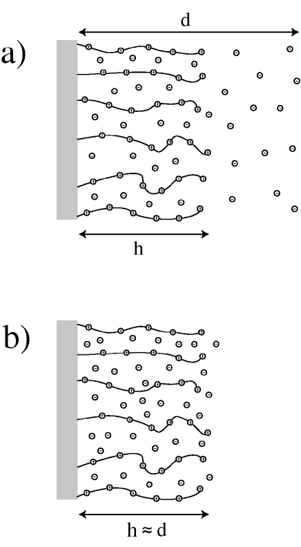
Figure 10: Schematic PE brush structure. In a) we show the weakly-charged limit where the counter-ion cloud has a thickness $d$ larger than the thickness of the brush layer, $h$. In b) we show the opposite case of the strongly-charged limit, where all counter-ions are contained inside the brush and a single length scale $d\approx h$ exists.

as a sum of separate contributions from the polyelectrolytes, $F_{\rm pol}$, contributions from the counterions, $F_{\rm ion}$, and an electrostatic interaction term $F_{\rm int}$ which couples polymers and counterions. The schematic geometry of the brush system is visualized in Figure 10: we assume that the charged brush is characterized by two length scales. The polymer chains are assumed to extend to a distance $h$ from the grafting surface, the counterions in general form a layer with a thickness of $d$. Two different scenarios emerge: The counter-ions can either extend outside the brush, $d\gg h$, as shown in Figure 10a, or be confined inside the brush, $d\approx h$ as shown in Figure 10b. As we demonstrate now, case b) is indicative of strongly charged brushes, and thus applicable to most experiments done on charged brushes so far, while case a) is typical for weakly charged brushes.

We recall that the grafting density of PE’s is denoted by $\rho_{a}$, $q$ is the counter-ion valency, $N$ the polymerization index of grafted chains, and $f$ the charge fraction. The counterion free energy contains entropic contributions (due to the confinement of the counterions inside a layer of thickness $d$) and also energetic contributions which come from interactions between counterions. In previous theories, a low-density expansion for the interaction part was used. We remind that the second-virial interaction is important for neutral brushes and is the driving repulsive force balancing the chain elasticity. For charged brushes, on the other hand, the leading term of the electrostatic correlation energy (which shows fractional scaling with respect to the charge density) is attractive and has been shown to lead to a collapse of the polyelectrolyte brush for large Bjerrum lengths[88, 89]. We will not pursue this collapse transition further in this review paper but solely concentrate on entropic and steric counterion effects, which is an acceptable approximation for mono-valent counterions.. In the present analysis we use a free-volume approximation very much in the spirit of the van-der-Waals equation for the liquid-gas transition. We include the effective hard-core volume of a single polyelectrolyte chain, which we call $V$, and which reduces the free volume that is available for the counterions. This free volume theory therefore takes the hard-core interactions between the polymer monomers and the counterions into account in a non-linear fashion and is valid even at large densities in the limit of close-packing. Compared to that, the excluded-volume interaction between counterions is small since the monomers are more bulky than the counterions and therefore it is neglected. The non-linear entropic free energy contribution of the counterions reads per unit area

$$F_{\rm ion}\simeq\frac{Nf\rho_{a}}{q}\left[\ln\left(\frac{Nf\rho_{a}/q}{d-\rho_{a}V}\right)-1\right]~{}.$$ (20)

In the limit of vanishing polymer excluded-volume, $V\rightarrow 0$, one recovers the standard ideal entropy expression. As the volume available for the counterions in the brush, which per polymer is just $d/\rho_{a}$, approaches the self volume of the polymers, $V$, the free energy expression Eq. (20) diverges, that means, the entropic prize for that scenario becomes infinitely large. The excluded volume of the polymers is roughly independent of the polymer brush height, and can be written in terms of the effective monomer hardcore diameter $\sigma_{\rm eff}$ and the polymer contour length $aN$ as $V\approx aN\sigma_{\rm eff}^{2}$. This leads to the final expression

$$F_{\rm ion}\simeq\frac{Nf\rho_{a}}{q}\left[\ln\left(\frac{Nf\rho_{a}/q}{d-Na\rho_{a}\sigma_{\rm eff}^{2}}\right)-1\right]~{}.$$ (21)

The polymer free energy $F_{\rm pol}$ per unit area can in principle be derived from the free energy per chain used for neutral brushes, Equation (12), by multiplying with the grafting density. It contains two contributions, one due to the chain elasticity and the other due to monomer-monomer interactions. Note that a logarithmic entropy term as for the counterions is missing, since the translational degrees of freedom of the monomers are lost due to chain connectivity. We recall that the entropy of chain stretching was accounted for by linear elasticity theory, with a spring constant proportional to $1/R_{0}^{2}$ in units of the thermal energy. This linear expression for the chain stretching is reliable for the neutral case, where indeed chain stretching is typically quite mild. For charged chains, the stretching is much stronger and we have to consider a more detailed model for the chain elasticity. For a freely jointed chain, which is a good model for synthetic polymer chains, the entropy loss due to stretching can be calculated exactly[90]. We only need here the asymptotic expressions for weak and for strong stretching, which read (per unit area)

$$F_{\rm pol}^{\rm el}\simeq\left\{\begin{array}[]{llll}&3\rho_{a}h^{2}/(2Na^{2})&{\rm for}&h\ll Na\\ &-\rho_{a}N\ln(1-h/Na)&{\rm for}&h\rightarrow Na\\ \end{array}\right.$$ (22)

and are proportional to the grafting density $\rho_{a}$. The contour length of the fully stretched chain is $Na$. The weak-stretching term is the standard term used in previous scaling models. For the highly stretched situations encountered in fully charged brushes, the strong-stretching term is typically more appropriate and leads to a few changes in the results as will be explained further below. The energetic contribution to the polymer free energy can be expressed as the second virial contribution, arising from steric repulsion between the monomers (contributions due to counter ions are neglected). Throughout this section, the polymers are assumed to be in a good solvent (positive second virial coefficient $v_{2}>0$). The contribution thus reads

$$F_{\rm pol}^{\rm en}\simeq\frac{1}{2}hv_{2}\left(\frac{N\rho_{a}}{h}\right)^{2}~{}.$$ (23)

An additional electrostatic component to the polymer interaction term is typically unimportant since the counterions strongly screen any Coulomb interactions[90]. Finally, an electrostatic interaction between polymers and counterions $F_{\rm int}$ occurs if the PE brush is not locally electro-neutral throughout the system, as for example is depicted in Fig. 10a. This energy is given by

$$F_{\rm int}=\frac{2\pi\ell_{\rm B}(Nf\rho_{a})^{2}}{3}\frac{(d-h)^{2}}{d}~{}.$$ (24)

This situation arises in the limit of low charge, when the counter-ion density profile extends beyond the brush layer, i.e. $d>h$.

The different free energy contributions lead, upon minimization with respect to the two length scales $h$ and $d$, to different behaviors. Let us first consider the weak charging limit, i.e.  the situation where the counter-ions leave the brush, $d>h$. In this case, minimization of ${F}_{\rm ion}+{F}_{\rm int}$ with respect to the counter-ion height $d$ in the limiting case of vanishing brush height ($h=0$) and monomer volume ($\sigma=0$) leads to

$$d=\frac{3}{2\pi q\ell_{B}Nf\rho_{a}}=3\lambda_{GC}$$ (25)

which has the same scaling as the so-called Gouy-Chapman length $\lambda_{GC}$. This length scale is a measure for the average height of the diffuse layer of $q$-valent counter-ions adsorbed at a surface with effective surface charge density $Nf\rho_{a}$ and has been determined within simulations and field-theory[91] but can also be obtained with more coarse-grained scaling arguments, as demonstrated here. Balancing now the polymer stretching energy ${F}_{\rm pol}^{\rm el}$ and the electrostatic energy ${F}_{\rm int}$ one obtains the so-called Pincus brush height

$$h\simeq N^{3}\rho_{a}\,a^{2}\ell_{B}f^{2}~{},$$ (26)

which results from the electrostatic attraction between the counter-ions and the charged monomers. One notes the peculiar dependence on the polymerization index $N$. In the limit of $d\approx h$, the PE brush can be considered as neutral and the electrostatic energy vanishes. There are two ways of balancing the remaining free energy contributions. The first is obtained by comparing the osmotic energy of counter-ion confinement, ${F}_{\rm ion}$, in the limit when $d=h$ and for vanishing polymer volume, with the polymer stretching term, ${F}_{\rm pol}^{\rm el}$, in the weak stretching limit, leading to the height

$$h\sim\frac{Naf^{1/2}}{(3q)^{1/2}}~{},$$ (27)

constituting the linear osmotic brush regime. The main assumption here is that all counterions stay strictly localized inside the brush, which will be tested later by comparison with computer simulations.

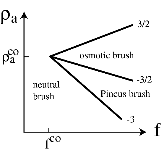
Figure 11: Scaling diagram for PE brushes on a log-log plot as a function of the grafting density $\rho_{a}$ and the fraction of charged monomers $f$. Featured are the Pincus-brush regime, where the counter-ion layer thickness is much larger than the brush thickness, the osmotic-brush regime, where all counter-ions are inside the brush and the brush height is determined by an equilibrium between the counter-ion osmotic pressure and the PE stretching energy, and the neutral-brush regime, where charge effects are not important and the brush height results from a balance of PE stretching energy and second-virial repulsion. The power law exponents of the various lines are denoted by numbers.

Finally comparing the second-virial term for the counterion interactions, ${F}_{\rm pol}^{\rm en}$, with the polymer stretching energy in the weak-stretching limit, ${F}_{\rm pol}^{el}$, one obtains the same scaling behavior as the neutral brush [21, 22], compare Eq.(13). Comparing the brush heights in all three regimes we arrive at the phase diagram shown in Fig. 11. The three scaling regimes coexist at the characteristic charge fraction

$$f^{\rm co}\sim\left(\frac{qv_{2}}{N^{2}a^{2}\ell_{B}}\right)^{1/3}~{},$$ (28)

and the characteristic grafting density

$$\rho_{a}^{\rm co}\sim\frac{1}{N\ell_{B}^{1/2}v_{2}^{1/2}}~{}.$$ (29)

4.2 Non-linear effects

The scaling relations for the brush height and the crossover boundaries between the various regimes constitute the simplest approach towards charged brushes. We pointed out already a few limitations of the presented results, which have to do with non-linear stretching and finite-volume effects.

Computer simulations provide an excellent mean to test those scaling relations. Extensive molecular dynamics simulations have been performed recently for polyelectrolyte brushes at various grafting densities and charge fractions, both at strong and intermediate electrostatic couplings[92, 93]. In these simulations, a freely-jointed bead-chain model is adopted for charged polymers end-grafted onto a rigid surface. The counterions are explicitly modeled as charged particles where both counterions and charged monomers are univalent and interact with the bare Coulomb potential Eq. (8). The strength of the Coulomb interaction is controlled by the Bjerrum length $\ell_{B}$. No additional electrolyte is added. The short-range repulsion between all particles is modeled by a shifted Lennard-Jones (LJ) potential, characterized by the hard-core diameter $\sigma$, as was done for the neutral brush simulations in Section 3.3. The simulation box is periodic in lateral directions and finite in the z-direction normal to the anchoring surface at z=0. We apply the techniques introduced by Lekner and Sperb to account for the long-range nature of the Coulomb interactions in a laterally periodic system [92]. To study the system in equilibrium we use stochastic molecular simulation at constant temperature.

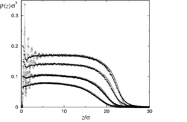
Figure 12: Density profiles of monomers (open symbols) and counterions (filled symbols) as a function of the distance from the anchoring surface. Shown are profiles for fully charged brushes of 36 chains of $N=30$ monomers at grafting densities (from bottom to top) $\rho_{\mathrm{a}}\sigma^{2}=0.042$ (circles), $0.063$ (squares), $0.094$ (diamonds), and $0.12$ (triangles). As can be clearly seen, the counterion stay inside the brush for all considered grafting densities and the local electroneutrality condition is satisfied very well.

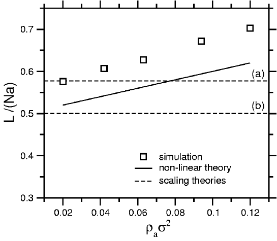
Figure 13: The circles show simulation data for the brush height as a function of grafting density for polyelectrolyte chains of $N=30$ monomers (contour length $L=30a$) with charge fraction of $f=1$. The Bjerrum length is $\ell_{B}=\sigma$, which corresponds to an intermediate coupling strength quite relevant for fully charged chains in water, and all ions are univalent. The dotted lines (a) and (b) show the linear scaling predictions, Eqs. (27) and (30), with Gaussian and non-linear elasticity respectively. The solid line shows the non-linear scaling prediction according to Eq. (31), which includes non-linear elasticity as well as the finite excluded volume of monomers and counterions.

Simulated density profiles of monomers and counterions of the system in normal direction are shown in Figure 12 for the fully charged brush at several grafting densities and for a Coulomb coupling characterized by $\ell_{B}/\sigma=1$, which is close to the coupling of monovalent ionic groups in water. As seen, both monomers and counterions follow very similar nearly-step-like profiles with uniform densities inside the brush, which increases with grafting density. These data show that the counterions are mostly confined in the brush layer and that the electroneutrality condition is satisfied locally. The simple explanation is that the Gouy-Chapman length is indeed very small and of the order or smaller than the monomer diameter. One can observe that the polyelectrolyte chains are stretched up to about 70 % of their contour length, which is roughly $L\approx N\sigma=30\sigma$, and thus their elastic behavior is far beyond the linear regime. Therefore, within the chosen range of parameters, the simulated brush is in the strong-charging (i.e., all counterions are confined within the brush) and strong-stretching limits; as we will show below, it exhibits a non-linear osmotic scaling behavior, so the linear scaling description of the last section, leading to Eq. (27), has to be slightly modified. The average height of end-points of the chains, $\langle z_{e}\rangle$, is one of the quantities which can be directly measured in the simulations and is shown in Figure 13 together with the predictions of the linear scaling theory, Eq. (27), denoted by (a), and the non-linear scaling predictions, to be explained further below. It is observed that the simulated brush height (solid circles) varies slowly with the grafting density, contrary to the prediction of the linear scaling theory, Eq.(27), but in agreement with recent experimental results[94, 95].

We now present a scaling theory that incorporates non-linear elastic and osmotic effects. In order to bring out the physics most clearly, the derivation will be done in two consecutive steps. First, in the strongly-stretched osmotic brush regime, one chooses the strong-stretching version of the chain-stretching entropy in Equation (22) and balances it with the counterion entropy, Equation (21), assuming vanishing polymer self volume, $\sigma=0$, and assuming equal heights for the brush and counterion layers, $d=h$. The result is

$$h\sim\frac{Naqf}{(1+qf)}~{},$$ (30)

which is the large-stretching analogue of Equation (27). The maximal stretching predicted from this equation is obtained for f=1 and corresponds to a vertical chain extension corresponding to 50 % of the contour length. For comparison, both expressions (27) and (30) are shown in Figure 13 as dashed lines (a) and (b) respectively. Still, the overall stretching is considerably smaller than what is observed in experiments and simulations, and it transpires that something is missing in the above scaling description. It has to do with the entropic pressure which increases as the volume within the brush is progressively more filled up by monomers and counterions. Note that the brush height in Equations (27) and (30) does not depend on the grafting density, in vivid contrast to the simulation results displayed in Figure 13.

In the non-linear osmotic brush regime we combine the high-stretching (non-linear) version of the chain elasticity in Equation (22) with the non-linear entropic effects of the counterions due to the finite volume of the polymer chains, i.e. we choose a finite polymer diameter $\sigma$ in Equation (21). The final result for the equilibrium brush height is

$$h\sim\frac{Na(qf+\sigma_{\rm eff}^{2}\rho_{a})}{(1+qf)}~{},$$ (31)

which in the limit of maximal grafting density, that is close packing, $\rho_{a}\rightarrow 1/\sigma^{2}_{\rm eff}$, reaches the maximal value stretching value, $h\rightarrow Na$, as one would expect: Compressing the brush laterally increases the vertical height and finally leads to a totally extended chain structure. In Figure 13, we compare expression Eq. (31) with the simulation results for the brush height as a function of grafting density. Note that we have used $\sigma_{\rm eff}^{2}=2\sigma^{2}$. This choice corresponds to an approximate two-dimensional square-lattice packing of monomers and counterions on two interpenetrating sublattices. As can be seen, the scaling prediction, Eq. (31), qualitatively captures the slow brush height increase with grafting density, as observed in the simulations. The deviations between simulation data and the non-linear osmotic brush prediction are unproblematic since the effective hard-core diameter of monomers in the simulation is difficult to determine precisely and might as well be treated as a fitting parameter. Deviations might also be explained by considering higher-order effects, such as lateral inhomogeneity of the counterion distribution around the brush chains and intermediate-stretching elasticity of the chains, that go beyond the present scaling analysis and have been considered in Ref.[90].

4.3 Additional effects

For large values of the charge fraction $f$ and the grafting density $\rho_{a}$, and for large Coulomb coupling, it has been found numerically that the brush height does not follow any of the scaling laws discussed here [92]. This has been recently rationalized in terms of another scaling regime, the collapsed regime. In this regime one finds that correlation and fluctuation effects, which are neglected in the discussion in this section, lead to a net attraction between charged monomers and counter-ions [88, 89].

If salt is present in the solution, counterions as well as co-ions do penetrate into the brush, which leads to additional screening of the Coulomb repulsion inside the brush. The amount of this screening, and the stretching of the polyectrolyte chains, are now also controlled by the bulk salt concentration. Since the additional salt screening weakens the swelling of the brush caused by the counterion osmotic pressure, salt leads to a brush contraction for sufficiently high salt concentration according to $h\sim c_{\rm salt}^{-1/3}$[76, 77]. The threshold salt concentration above which the brush contraction sets in is given by the salt concentration which equals the counterion concentration inside the brush. This means that the higher the grafting density (and consequently the higher the internal counterion concentration in the osmotic brush regime), the larger the salt concentration neceassary to see any salt effects at all.

Another way of creating a charged brush is to dissolve a diblock copolymer consisting of a hydrophobic and a charged block in water. The diblocks associate to form a hydrophobic core, thereby minimizing the unfavorable interaction with water, while the charged blocks form a highly charged corona or brush [96]. The micelle morphology depends on different parameters. Most importantly, it can be shown that salt acts as a morphology switch, giving rise to the sequence spherical, cylindrical, to planar micellar morphology as the salt concentration is increased [96]. Theoretically, this can be explained by the entropy cost of counter-ion confinement in the charged corona [97]. The charged corona can be studied by neutron scattering [98] or atomic-force microscopy [99] and gives information on the behavior of highly curved charged brushes.

5 Concluding Remarks

In this short review about neutral and charged polymers that are terminally grafted with one end to a surface we tried to explain and contrast the most important theoretical methods used for their understanding and description. The theories used for brushes are quite different from ordinary polymer modelling since the statistics of the grafted layer depends crucially on the fact that the chain is not attracted to the surface but is forced to be in contact to the surface since one of its ends is chemically or physically bonded to the surface. We review scaling concepts, mean–field theory and simulation techniques that give information on brushes on different levels of detail and accuracy. Scaling concepts yield the qualitative features of brushes, i.e. the brush height and its free energy as a function of the main parameters and without reliable prefactors. Mean-field or self-consistent theories allow to construct density distributions on a coarse grained level, but correlation effects are completely missed. Simulation techniques give in principle exact numerical results for the case of so-called primitive models where the solvent is neglected and monomers and ions are modeled as charged soft spheres. Current open questions concern the structure of water in such dense systems: is water still described by a continuous medium with the bulk dielectric constant? Secondly, all approaches neglect the varying polarizability of the monomers and ions, which again give rise to pronounced image-charge effects in the brush geometry. Lastly, most brush systems have not reached their true equilibrium structure, so that we are in essence dealing with an non-equilibrium system. How do we describe such non-equilibrium systems, and what governs the approach towards equilibrium including hydrodynamic and local friction effects? We believe that the triad of scaling, field-theoretic, and simulation techniques will also allow to gain understanding of these more complicated issues in the near future.

6 References

References

- [1] Yamakawa H (1971) Modern Theory of Polymer Solutions, Harper & Row, New York
- [2] de Gennes PG (1979) Scaling Concepts in Polymer Physics, Cornell University, Ithaca
- [3] Grosberg AY, Khokhlov AR (1994) Statistical Physics of Macromolecules, AIP Press, New York
- [4] Rubinstein M (2003) Polymer Physics, Oxford University Press, Oxford
- [5] Netz RR, Andelman D (2003) Physics Reports 380:1
- [6] Halperin A, Tirell M, Lodge TP (1992) Adv Pol Sc 100:31
- [7] Szleifer I, Carignano MA (1996) Adv Chem Phys XCIV:165
- [8] Taunton HJ, Toprakcioglu C, Fetters LJ, Klein J (1988) Nature 332:712; (1990) Macromolecules 23:571
- [9] Auroy P, Auvray L, Leger L (1991) Phys Rev Lett 66:719; (1991) Macromolecules 24:2523; (1991) Macromolecules 24:5158
- [10] Marques CM, Joanny JF, Leibler L (1988) Macromolecules 21:1051; Marques CM, Joanny JF (1989) Macromolecules 22:1454
- [11] Field JB, Toprakcioglu C, Dai L, Hadziioannou G, Smith G, Hamilton W (1992) J Phys II France 2:2221
- [12] Kent MS, Lee LT, Factor BJ, Rondelez F, Smith GS (1995) J Chem Phys 103:2320
- [13] Bijsterbosch HD, de Haan VO, de Graaf AW, Mellema M, Leermakers FAM, Cohen Stuart MA, van Well AA (1995) Langmuir 11:4467
- [14] Teppner R, Motschmann H (1998) Macromolecules 31:7467
- [15] Oosawa F (1971) Polyelectrolytes, Dekker, New York
- [16] Förster S, Schmidt M (1995) Adv Polym Sci 120:50
- [17] Barrat JL, Joanny JF (1996) Adv Chem Phys 94:1
- [18] Holm H, Joanny JF, Kremer K, Netz RR, Reineker P, Seidel C, Vilgis TA, Winkler RG (2004) Adv Polym Science 166:67
- [19] Rühe J, Ballauff M, Biesalski M, Dziezok P, Gröhn F, Johannsmann D, Houbenov N, Hugenberg N, Konradi R, Minko S, Motornov M, Netz RR, Schmidt M, Seidel C, Stamm M, Stephan T, Usov D, Zhang H (2004) Adv Polym Science 165:79
- [20] Dolan AK, Edwards SF (1974) Proc R Soc Lond A 337:509; 343:427
- [21] Alexander S (1977) J Phys (France) 38:983
- [22] de Gennes PG (1980) Macromolecules 13:1069
- [23] Semenov AN (1985) Sov Phys JETP 61:733
- [24] Daoud M, Cotton JP (1982) J Phys France 43:531
- [25] Karim A, Satija SK, Douglas JF, Ankner JF, Fetters LJ (1994) Phys Rev Lett 73: 3407
- [26] Baltes H, Schwendler M, Helm CA, Heger R, Goedel WA (1997) Macromolecules 30:6633
- [27] Netz RR (2003) J Phys: Condens Mat 15:S239
- [28] Burak Y, Netz RR (2004) J of Chem Phys B 108:4840
- [29] Odijk T (1977) J Polym Sci, Polym Phys Ed 15:477; (1978) Polymer 19:989
- [30] Skolnick J, Fixman M (1977) Macromolecules 10:944
- [31] Barrat JL, Joanny JF (1993) Europhys Lett 24:333
- [32] Netz RR, Orland H (1999) Eur Phys J B 8:81
- [33] Manghi M, Netz RR (2004) Eur Phys J E 14:67
- [34] Ullner M, Woodward CE (2002) Macromolecules 35:1437
- [35] Everaers R, Milchev A, Yamakov V (2002) Eur Phys J E 8:3
- [36] Netz RR, Joanny JF (1999) Macromolecules 32: 9013; Netz RR, Joanny JF (1999) Macromolecules 32: 9026
- [37] Manning GS (1969) J Chem Phys 51:924
- [38] Manning GS (1969) J Chem Phys 51:934
- [39] Manning GS, Ray J (1998) J Biomol Struct Dyn 16:461
- [40] Fixman M (1982) J Chem Phys 76:6346
- [41] Le Bret M (1982) J Chem Phys 76:6243
- [42] Manning GS, Mohanty U (1997) Physica A 247:196
- [43] Manning GS (1988) J Chem Phys 89:3772
- [44] Wandrey C, Hunkeler D, Wendler U, Jaeger W (2000) Macromolecules 33:7136
- [45] Blaul J, Wittemann M, Ballauff M, Rehahn M (2000) J Phys Chem B 104:7077
- [46] Cosgrove T, Heath T, van Lent B, Leermakers FAM, Scheutjens J (1987) Macromolecules 20:1692
- [47] Murat M, Grest GS (1989) Macromolecules 22:4054; Chakrabarti A, Toral R (1990) Macromolecules 23:2016; Lai PY, Binder K (1991) J Chem Phys 95:9288
- [48] Milner ST, Witten TA, Cates ME (1988) Europhys Lett 5:413; (1988) Macromolecules 21:610
- [49] Skvortsov AM, Pavlushkov IV, Gorbunov AA, Zhulina YB, Borisov OV, Pryamitsyn VA (1988) Polymer Science 30:1706
- [50] Netz RR, Schick M (1997) Europhys Lett 38:37; (1998) Macromolecules 31:5105
- [51] Carignano MA, Szleifer I (1995) J Chem Phys 102:8662
- [52] Martin JI, Wang ZG (1995) J Chem Phys 99:2833
- [53] Baranowski R, Whitmore MD (1995) J Chem Phys 103:2343
- [54] Currie EPK, Leermakers FAM, Cohen Stuart MA, Fleer GJ (1999) Macromolecules 32:487
- [55] Grest GS (1994) Macromolecules 27:418
- [56] Seidel C, Netz RR (2000) Macromolecules 33:634
- [57] Witten TA, Pincus PA (1986) Macromolecules 19:2509; Zhulina EB, Borisov OV, Priamitsyn VA (1990) J Coll Surf Sci 137:495
- [58] Milner ST (1988) Europhys Lett 7:695
- [59] Milner ST, Witten TA, Cates ME (1989) Macromolecules 22:853
- [60] Halperin A (1988) J Phys France 49:547; Zhulina EB, Borisov OV, Pryamitsyn VA, Birshtein TM (1991) Macromolecules 24:140; Williams DRM (1993) J Phys II France 3:1313
- [61] Auroy P, Auvray L (1992) Macromolecules 25:4134
- [62] Marko JF (1993) Macromolecules 26:313
- [63] Lai PY, Binder K (1992) J Chem Phys 97:586; Grest GS, Murat M (1993) Macromolecules 26:3108
- [64] Ball RC, Marko JF, Milner ST, Witten TA (1991) Macromolecules 24:693; Li H, Witten TA (1994) Macromolecules 27:449; Manghi M, Aubouy M, Gay C, Ligoure C (2001) Eur Phys J E 5:519
- [65] Dan N, Tirrell M (1992) Macromolecules 25:2890
- [66] Murat M, Grest GS (1991) Macromolecules 24:704
- [67] Milner ST, Witten TA (1988) J Phys France 49:1951
- [68] Aubouy M, Fredrickson GH, Pincus P, Raphael E (1995) Macromolecules 28:2979
- [69] Gast AP, Leibler L (1986) Macromolecules 19:686
- [70] Borukhov I, Leibler L (2000) Phys Rev E 62:R41
- [71] Marko JF, Witten TA (1991) Phys Rev Lett 66:1541
- [72] Brown G, Chakrabarti A, Marko JF (1995) Macromolecules 28:7817; Zhulina EB, Singhm C, Balazs AC (1996) Macromolecules 29:8254
- [73] Halperin A, Alexander S (1988) Europhys Lett 6:329; Johner A, Joanny JF (1990) Macromolecules 23:5299; Ligoure C, Leibler L (1990) J Phys France 51:1313; Milner ST (1992) Macromolecules 25:5487; Johner A, Joanny JF (1993) J Chem Phys 98:1647
- [74] Miklavic SJ, Marcelja S (1988) J Phys Chem 92:6718
- [75] Misra S, Varanasi S, Varanasi PP (1989) Macromolecules 22:5173
- [76] Pincus P (1991) Macromolecules 24:2912
- [77] Borisov OV, Birstein TM, Zhulina EB (1991) J Phys II (France) 1:521
- [78] Ross RS, Pincus P (1992) Macromolecules 25:2177; Zhulina EB, Birstein TM, Borisov OV (1992) J Phys II (France) 2:63
- [79] Wittmer J, Joanny JF (1993) Macromolecules 26:2691
- [80] Israels R, Leermakers FAM, Fleer GJ, Zhulina EB (1994) Macromolecules 27:3249
- [81] Borisov OV, Zhulina EB, Birstein TM (1994) Macromolecules 27:4795
- [82] Zhulina EB, Borisov OV (1997) J Chem Phys 107:5952
- [83] Mir Y, Auvroy P, Auvray L (1995) Phys Rev Lett 75:2863
- [84] Guenoun P, Schlachli A, Sentenac D, Mays JM, Benattar JJ (1995) Phys Rev Lett 74:3628
- [85] Ahrens H, Förster S, Helm CA (1997) Macromolecules 30:8447; (1998) Phys Rev Lett 81:4172
- [86] Ballauff M, Guo X (2001) Phys Rev E 64:051406
- [87] Balastre M, Li F, Schorr P, Yang J, Mays JW, Tirrell MV (2002) Macromolecules 35:9480.
- [88] Csajka FS, Netz RR, Seidel C, Joanny JF (2001) Eur Phys J E 4:505
- [89] Santangelo CD, Lau AWC (2004) Eur Phys J E 13:335
- [90] Naji A, Netz RR, Seidel C (2003) Eur Phys J E 12:223
- [91] Moreira AG, Netz RR (2001) Phys Rev Lett 87:078301; (2002) Eur Phys J E 8:33
- [92] Csajka F, Seidel C (2000) Macromolecules 33:2728
- [93] Seidel C (2003) Macromolecules 36:2536
- [94] Romet-Lemonne, Daillant J, Guenoun P, Yang J, Mays JW (2004) to be published
- [95] Ahrens H, Förster S, Helm CA, Naji A, Netz RR, Seidel C (2004) J Chem Phys in press
- [96] Shen H, Zhang L, Eisenberg A (1999) J Am Chem Soc 121:2728
- [97] Netz RR (1999) Europhys Lett 47:391
- [98] Guenoun P, Muller F, Delsanti M, Auvray L, Chen YJ, Mays JW, Tirrell M (1998) Phys Rev Lett 81:3872; Guenoun P, Delsanti M, Gazeau D, Mays JW, Cook DC, Tirrell M, Auvray L (1998) Eur Phys J B 1: 77
- [99] Förster S, Hermsdorf N, Leube W, Schnablegger H, Regenbrecht M, Akarai S, Lindner P, Böttcher C (1999) J Phys Chem B 103:6657