.

STRONG-COUPLING THEORY

OF HIGH TEMPERATURE SUPERCONDUCTIVITY

A.S. Alexandrov

Loughborough University, Loughborough LE11 3TU, United Kingdom

INTRODUCTION

The seminal work by Bardeen, Cooper and Schrieffer (BCS)bcs extended further by Eliashberg eli to the intermediate coupling regime solved one of the major scientific problems of Condensed Matter Physics in the last century. While the BCS theory provides a qualitatively correct description of some novel superconductors like magnesium diboride and doped fullerenes, if the phonon dressing of carriers (i.e. polaron formation) is properly taken into account, high-temperature superconductivity (HTS) of cuprates represents a challenge to the conventional theory. Here I discuss a multi-polaron approach to the problem based on our extension of the BCS theory to the strong-coupling regime alebook1 . Attractive electron correlations, prerequisite to any HTS, are caused by an almost unretarded electron-phonon (e-ph) interaction sufficient to overcome the direct Coulomb repulsion in this regime. Low energy physics is that of small polarons and bipolarons (real-space electron (hole) pairs dressed by phonons). They are itinerant quasiparticles existing in the Bloch states at temperatures below the characteristic phonon frequency. Since there is almost no retardation (i.e. no Tolmachev-Morel-Anderson logarithm) reducing the Coulomb repulsion, e-ph interactions should be relatively strong to overcome the direct Coulomb repulsion, so carriers must be polaronic to form pairs in novel superconductors. I identify the Fröhlich electron-phonon interaction as the most essential for pairing in superconducting cuprates. Many experimental observations have been satisfactorily understood in the framework of the bipolaron theory alebook1 providing evidence for a novel state of electronic matter in layered cuprates, which is a charged Bose-liquid of small mobile bipolarons.

Here the band structure and essential interactions in oxide superconductors are discussed in section 1, and the ”Fröhlich-Coulomb” model of HTS is introduced in section 2, including discussions of single-polaron (2.1, 2.2, 2.3, 2.4, 2.5) and multipolaron (2.4, 2.6, 3.1, 3.2) problems, low-energy structures (3.3), and the phase diagram of cuprates (3.4). ”Individual” versus Cooper pairing (3.5), normal state properties (section 4), in particular in-plane resistivity, the Hall effect, magnetic susceptibility and the Lorenz number (4.1), the Nernst effect (4.2), diamagnetism (4.3), spin and charge pseudogaps, and c-axis transport (4.4) are also discussed. I present a parameter-free evaluation of $T_{c}$ (5.1), and an explanation of isotope effects (5.2), specific heat anomaly (5.3), upper critical fields (5.4), symmetries and space modulations of the order parameter (5.5), and a model of overdoped cuprates as mixtures of mobile bipolarons and degenerate lattice polarons (section 6).

I Band structure and essential interactions in cuprates

A significant fraction of theoretical research in the field of HTS has suggested that the interaction in novel superconductors is essentially repulsive and unretarded, and it could provide high $T_{c}$ without phonons. Indeed strong on-site repulsive correlations (Hubbard $U$) are essential in shaping the insulating state of undoped (parent) compounds. Different from conventional band-structure insulators with completely filled and empty Bloch bands, the Mott insulator arises from a potentially metallic half-filled band as a result of the Coulomb blockade of electron tunnelling to neighboring sites mott .

In our approach to cuprate superconductors we take the view that cuprates and related transition metal oxides are charge-transfer Mott-Hubbard insulators at $any$ relevant level of doping alebook1 . The one-particle density-of-states (DOS) of cuprates is schematically represented by Fig.1, as it has been established in a number of site-selective experiments sel and in the first-principle numerical (”LDA+U”) first and semi-analytical cluster ovc band structure calculations properly taking into account the strong on-site repulsion. Here d-band of the transition metal (Cu) is split into the lower and upper Hubbard bands by the on-site repulsive interaction $U$, while the first band to be doped is an oxygen band within the Hubbard gap. The oxygen band is less correlated and completely filled in parent insulators, so a single oxygen hole has well defined quasi-particle properties in the absence of interactions with phonons and with spin fluctuations of d-band electrons.

Unfortunately, the Hubbard $U$ model shares an inherent difficulty in determining the order when the Mott-Hubbard insulator is doped. While some groups have claimed that it describes high-$T_{c}$ superconductivity at finite doping, other authors could not find any superconducting instability. Therefore it has been concluded that models of this kind are highly conflicting and confuse the issue by exaggerating the magnetism rather than clarifying it lau . The Hubbard-$U$ model of HTS and its strong-coupling $"t-J"$ approximation pla are also refutable on experimental ground. A characteristic magnetic interaction, which is allegedly responsible for pairing in the model, is the spin-exchange interaction, $J=4t^{2}/U$, of the order of $0.1$ eV (here $t$ is the hopping integral). On the other hand, a simple parameter-free estimate of the Fröhlich electron-phonon interaction (routinely neglected within the Hubbard $U$ approach) yields the effective attraction as high as $1$ eV alebook1 . This estimate is obtained using the familiar expression for the polaron level shift, $E_{p},$ the high-frequency, $\epsilon_{\infty}$, and the static, $\epsilon_{0},$ dielectric constants of the host insulator, measured experimentally alebra1 ,

$$E_{p}={\frac{1}{{2\kappa}}}\int_{BZ}{\frac{d^{3}q}{{(2\pi)^{3}}}}{\frac{4\pi e^{2}}{{q^{2}}}},$$ (1)

where $\kappa^{-1}=\epsilon_{\infty}^{-1}-\epsilon_{0}^{-1}$ and the size of the integration region is the Brillouin zone (BZ).

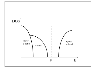
Figure 1: DOS in cuprates. The chemical potential $\mu$ is inside the charge transfer gap as observed in the tunnelling experiments boz0 because of bipolaron formation alebook1 . It could enter the oxygen band in overdoped cuprates, if bipolarons coexist with unpaired degenerate polarons (section 6).

Since $\epsilon_{\infty}=5$ and $\epsilon_{0}=30$ in La₂CuO₄ one obtains $E_{p}=0.65$ eV. Hence the attraction, which is about $2E_{p}$, induced by the long-range lattice deformation in parent cuprates is one order of magnitude larger than the exchange magnetic interaction. There is virtually no screening of e-ph interactions with $c-$axis polarized optical phonons in doped cuprates because the upper limit for an out-of-plane plasmon frequency ($<200$ cm^-1)mar1 is well below characteristic phonon frequencies, $\omega\approx$ 400 - 1000 cm ^-1 . Hence the Fröhlich interaction remains the most essential pairing interaction at any doping.

Further compelling evidence for the strong e-ph interaction has come from isotope effects zhao , more recent high resolution angle resolved photoemission spectroscopies (ARPES) LAN , and a number of earlier optical mic1 ; ita ; tal ; tim and neutron-scattering ega studies of cuprates. The strong coupling with optical phonons, unambiguously established in all high-temperature superconductors, transforms holes into lattice mobile polarons and mobile superconducting bipolarons as has been proposed alerun prior the discovery mul ; chu .

When the e-ph interaction binds holes into intersite oxygen bipolarons alebook1 , the chemical potential remains pinned inside the charge transfer gap. It is found at a half of the bipolaron binding energy, Fig.1, above the oxygen band edge shifted by the polaron level shift $E_{p}$, as clearly observed in the tunnelling experiments by Bozovic et al. in optimally doped La_1.85Sr_0.15 Cu O₄ boz0 . The bipolaron binding energy as well as the singlet-triplet bipolaron exchange energy (section 3) are thought to be the origin of normal state charge and spin pseudogaps, respectively, as has been proposed by us alegap and later found experimentally kabmic . In overdoped samples carriers screen part of the e-ph interaction with low frequency phonons. Hence, the bipolaron binding energy decreases alekabmot and the hole bandwidth increases with doping. As a result, the chemical potential could enter the oxygen band in overdoped samples because of an overlap of the bipolaron and polaron bands, so a Fermi-level crossing could be seen in ARPES (section 6).

II ”Fröhlich-Coulomb” model of HTS

Experimental facts tell us that any realistic description of high temperature superconductivity should treat the long-range Coulomb and unscreened e-ph interactions on an equal footing. In the past decade we have developed a ”Fröhlich-Coulomb” model (FCM) ale5 ; alebook1 ; alekor to deal with the strong long-range Coulomb and the strong long-range e-ph interactions in cuprates and other related compounds. The model Hamiltonian explicitly includes a long-range electron-phonon and the Coulomb interactions as well as the kinetic and deformation energies. The implicitly present large Hubbard $U$ term prohibits double occupancy and removes the need to distinguish fermionic spins since the exchange interaction is negligible compared with the direct Coulomb and the electron-phonon interactions.

Introducing spinless fermionic, $c_{\bf n}$, and phononic, $d_{{\bf m}\alpha}$, operators the Hamiltonian of the model is written as

$$H= - \sum_{\bf n\neq n^{\prime}}\left[T({\bf n-n^{\prime}})c_{\bf n}^{\dagger}c_{\bf n^{\prime}}-V_{c}({\bf n-n^{\prime}})c_{\bf n}^{\dagger}c_{\bf n}c_{\bf n^{\prime}}^{\dagger}c_{\bf n^{\prime}}\right]$$ (2)

$$- \sum_{\alpha,\bf nm}\omega_{\alpha}g_{\alpha}({\bf m-n})({\bf e}_{\alpha}\cdot{\bf u}_{\bf m-n})c_{\bf n}^{\dagger}c_{\bf n}(d_{{\bf m}\alpha}^{\dagger}+d_{{\bf m}\alpha})$$

$$+ \sum_{{\bf m}\alpha}\omega_{\alpha}\left(d_{{\bf m}\alpha}^{\dagger}d_{{\bf m}\alpha}+1/2\right),$$

where $T({\bf n})$ is the hopping integral in a rigid lattice, ${\bf e}_{\alpha}$ is the polarization vector of the $\alpha$th vibration coordinate, ${\bf u}_{\bf m-n}\equiv({\bf m-n})/|{\bf m-n}|$ is the unit vector in the direction from electron ${\bf n}$ to ion ${\bf m}$, $g_{\alpha}({\bf m-n)}$ is the dimensionless e-ph coupling function, and $V_{c}({\bf n-n^{\prime}})$ is the inter-site Coulomb repulsion. $g_{\alpha}({\bf m-n)}$ is proportional to the force acting between the electron on site ${\bf n}$ and the ion on ${\bf m}$. For simplicity, we assume that all the phonon modes are non-dispersive with the frequency $\omega_{\alpha}$. We also use $\hbar=k_{B}=c=1$.

If the electron-phonon interaction is strong, i.e. the conventional e-ph coupling constant of the BCS theory is large, $\lambda>1$, then the weak-coupling BCS bcs and the intermediate-coupling Migdal-Eliashberg mig ; eli approaches cannot be applied alebreak . Nevertheless the Hamiltonian, Eq.(2), can be solved analytically by using the $"1/\lambda"$ multi-polaron expansion technique alebook1 , if $\lambda=E_{p}/zT(a)>1$. Here the polaron level shift is

$$E_{p}=\sum_{{\bf n}\alpha}\omega_{\alpha}g_{\alpha}^{2}({\bf n})({\bf e}_{\alpha}\cdot{\bf u}_{\bf n})^{2},$$ (3)

and $zT(a)$ is about the half-bandwidth in a rigid lattice. As I discuss below, the model shows a rich phase diagram depending on the ratio of the inter-site Coulomb repulsion $V_{c}$ and the polaron level shift $E_{p}$ alekor . The ground state of FCM is a polaronic Fermi liquid when the Coulomb repulsion is large, a bipolaronic high-temperature superconductor at intermediate Coulomb repulsions, and a charge-segregated insulator if the repulsion is weak. FCM predicts superlight polarons and bipolarons in cuprates with a remarkably high superconducting critical temperature. Cuprate bipolarons are relatively light because they are inter-site rather than on-site pairs due to the strong on-site repulsion, and because mainly $c$-axis polarized optical phonons are responsible for the in-plane mass renormalization. The relatively small mass renormalization of polaronic and bipolaronic carries in FCM has been confirmed numerically using the exact QMC Korn2 , cluster diagonalization feh3 and variational bon2 simulations.

(Bi)polarons describe many properties of cuprates alebook1 , in particular normal-state transport (section 4), including in-plane and out-of-plane resistivity, the Hall effect, spin susceptibility, thermal conductivity, normal state pseudogaps, the Nernst effect, normal state diamagnetism, superconducting transition, including high values of $T_{c}$, isotope effects, unusual upper critical fields, symmetries and real-space modulations of the superconducting order parameter (section 5).

II.1 Single lattice polaron

Let us first discuss a single lattice-polaron problem. Conducting electrons in inorganic and organic matter interact with vibrating ions. If phonon frequencies are sufficiently low, the local deformation of ions, caused by electron itself, creates a potential well, which traps the electron even in a perfect crystal lattice. This self-trapping phenomenon was predicted by Landau land . It was studied in greater detail by Pekar pek , Fröhlich fro , Feynman fey , Rashba ras , Devreesedev and other authors in the effective mass approximation for the electron placed in a continuous polarizable medium, which leads to a so-called large or continuous polaron. Large polaron wave functions and corresponding lattice distortions spread over many lattice sites. The trapping is never complete in the perfect lattice. Due to finite phonon frequencies ion polarizations follow polaron motion if the motion is sufficiently slow. Hence, large polarons with a low kinetic energy propagate through the lattice as free electrons but with an enhanced effective mass.

When the electron-phonon (e-ph) interaction energy $E_{p}$ is compared with the electron energy-bandwidth, all electrons in the Bloch bands of the crystal are “dressed” by phonons. In this strong-coupling regime, $\lambda=E_{p}/D>1,$ the finite bandwidth $2D$ becomes important, so the continuous approximation cannot be applied. The main features of small polarons were understood by Tjablikov tja , Yamashita and Kurosava yam , Sewell sew , Holstein hol and his school, Lang and Firsov lan , Eagles eag , and by other researches and described in several review papers and textbooks small . The polaron shift of the atomic level and an exponential reduction of the bandwidth (see below) at large values of $\lambda$ are among those features. The shift can be easily understood using a toy model of an electron localized on site n and interacting with a single ion vibrating near site m in the direction connecting n and m, Fig.2. The vibration part of the Hamiltonian in this toy model is

$$H_{ph}=-{1\over{2M}}{\partial^{2}\over{\partial x^{2}}}+{kx^{2}\over{2}},$$ (4)

where $M$ is the ion mass, $k=M\omega^{2}$ is the spring constant, and $x$ is the ion displacement. The electron potential energy due to its Coulomb interaction with the ion is approximately

$$V=V_{0}(1-x/a),$$ (5)

where $V_{0}=-Ze^{2}/a$ is the Coulomb energy in a rigid lattice (an analog of the crystal field potential), and $a$ is the average distance between sites. Hence the Hamiltonian of the model is given by

$$H=E_{a}\hat{n}+fx\hat{n}-{1\over{2M}}{\partial^{2}\over{\partial x^{2}}}+{kx^{2}\over{2}},$$ (6)

where $E_{a}$ is the atomic level at site ${\bf m}$ in the rigid lattice, which includes the crystal field, $f=Ze^{2}/a^{2}$ is the Coulomb force, and $\hat{n}=c^{\dagger}c$ is the occupation number operator on site ${\bf n}$ expressed in terms of the electron annihilation $c$ and creation $c^{\dagger}$ operators. This Hamiltonian can be readily diagonals using a displacement transformation of the vibration coordinate $x$,

$$x=y-\hat{n}f/k.$$ (7)

The transformed Hamiltonian has no electron-phonon coupling,

$$\tilde{H}=(E_{a}-E_{p})\hat{n}-{1\over{2M}}{\partial^{2}\over{\partial y^{2}}}+{ky^{2}\over{2}},$$ (8)

where we used $\hat{n}^{2}=\hat{n}$ because of the Fermi statistics. It describes a small polaron at the atomic level, shifted by the polaron level shift $E_{p}=f^{2}/2k$, and entirely decoupled from ion vibrations. The ion vibrates near a new equilibrium, shifted by $f/k$, with the ”old” frequency $\omega$. As a result of the local ion deformation, the total energy of the whole system decreases by $E_{p}$ since a decrease of the electron energy by $-2E_{p}$ overruns an increase of the deformation energy $E_{p}$.

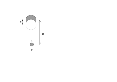
Figure 2: Localized electron shifts the equilibrium position of an ion and lowers the atomic energy level.

The tunnelling of small polarons in the lattice can be understood within a simple Holstein model hol consisting of two molecules and a single electron. Here I slightly simplify the original Holstein model replacing two molecules by two rigid sites $1$ (”left”) and $2$ (”right”) with the hopping amplitude $t$ between them. The electron interacts with a vibrational mode of an ion, placed at some distance in between, Fig.3, rather than with the intra-molecular vibrations:

$$H=t(c_{1}^{\dagger}c_{2}+c_{2}^{\dagger}c_{1})+H_{ph}+H_{e-ph},$$ (9)

where $H_{e-ph}$ depends on the polarization of vibrations, and $E_{a}=0$ is taken. If the ion vibrates along the perpendicular direction to the hopping (in ”c”-direction) we have

$$H_{e-ph}=f_{c}x(c_{1}^{\dagger}c_{1}+c_{2}^{\dagger}c_{2}),$$ (10)

and

$$H_{e-ph}=f_{a}x(c_{1}^{\dagger}c_{1}-c_{2}^{\dagger}c_{2}),$$ (11)

if the ion vibrates along the hopping (”a” direction).

The wave-function of the electron and the ion is a linear superposition of two terms describing the electron on the ”left” and on the ”right” site, respectively,

$$\psi=[u(x)c_{1}^{\dagger}+v(x)c_{2}^{\dagger}]|0\rangle,$$ (12)

where $|0\rangle$ is the vacuum state describing a rigid lattice without the extra electron. Substituting $\psi$ into the Schrödinger equation, $H\psi=E\psi$, we obtain two coupled equations for the amplitudes,

$$(E-f_{a,c}x-H_{ph})u(x)=tv(x),$$ (13)

$$(E\pm f_{a,c}x-H_{ph})v(x)=tu(x).$$ (14)

Figure 3: Electron tunnels between sites $1$ (”left”) and $2$ (”right”) with the amplitude $t$ and interacts with c-axis or a-axis polarized vibrational modes of the ion, placed in between.

There is the exact solution for the ”c”-axis polarization, when a change in the ion position leads to the same shift of the electron energy on the left and on the right sites,

$$u(x)=u\chi_{n}(x),$$

$$v(x)=v\chi_{n}(x),$$ (15)

where $u$ and $v$ are constants and

$$\chi_{n}(x)=\left(\frac{M\omega}{\pi(2^{n}n!)^{2}}\right)^{1/4}H_{n}[(x-f_{c}/k)(M\omega)^{1/2}]\exp[-M(x-f_{c}/k)^{2}\omega/2],$$ (16)

is the harmonic oscillator wave-function. There are two ladders of levels given by

$$E^{\pm}_{n}=-E_{p}\pm t+\omega(n+1/2)$$ (17)

with $E_{p}=f_{c}^{2}/2k$. Here

$$H_{n}(\xi)=(-1)^{n}e^{\xi^{2}}\frac{d^{n}e^{-\xi^{2}}}{d\xi^{n}}$$ (18)

are the Hermite polynomials, and $n=0,1,2,3,...$ . Hence the c-axis single-ion deformation leads to the polaron level shift but without any renormalization of the hopping integral $t$. In contrast, $a$-polarized vibrations with the opposite shift of the electron energy on the left and on the right sites, strongly renormalize the hopping integral. There is no simple general solution of the Holstein model in this case, but one can find it in two limiting cases, $nonadiabatic$, when $t\ll\omega$ and $adiabatic$, when $t\gg\omega$.

II.2 Non-adiabatic small polaron

In the non-adiabatic regime the ion vibrations are fast and the electron hopping is slow. Hence one can apply a perturbation theory in powers of $t$ to solve

$$\left(\begin{array}[]{cc}E-f_{a}x-H_{ph}&-t\\ -t&E+f_{a}x-H_{ph}\\ \end{array}\right)\left(\begin{array}[]{c}u(x)\\ v(x)\\ \end{array}\right)=0.$$ (19)

We take $t=0$ in zero order, and obtain a two-fold degenerate ground state $[u^{l,r}(x),v^{l,r}(x)]$, corresponding to the polaron localized on the left ($l$) or on the right ($r$) sites,

$$u^{l}(x)=exp\left[-{M\omega\over{2}}(x+f_{a}/k)^{2}\right],$$ (20)

$$v^{l}(x)=0$$ (21)

and

$$u^{r}(x)=0,$$ (22)

$$v^{r}(x)=exp\left[-{M\omega\over{2}}(x-f_{a}/k)^{2}\right]$$ (23)

with the energy $E_{0}=-E_{p}+\omega/2$, where $E_{p}=f_{a}^{2}/2k$. The eigenstates are found as linear superpositions of two unperturbed states,

$$\left(\begin{array}[]{c}u(x)\\ v(x)\\ \end{array}\right)=\alpha\left(\begin{array}[]{c}u^{l}(x)\\ 0\\ \end{array}\right)+\beta\left(\begin{array}[]{c}0\\ v^{r}(x)\\ \end{array}\right).$$ (24)

Here the coefficients $\alpha$ and $\beta$ are independent of $x$. The conventional secular equation for $E$ is obtained, multiplying the first row by $u^{l}(x)$ and the second row by $v^{r}(x)$, and integrating over the vibration coordinate, $x$, each of two equations of the system. The result is

$$\det\left(\begin{array}[]{cc}E-E_{0}&\tilde{t}\\ \tilde{t}&E-E_{0}\\ \end{array}\right)=0$$ (25)

with the renormalized hopping integral

$${\tilde{t}\over{t}}={\int^{\infty}_{-\infty}dxu^{l}(x)v^{r}(x)\over{\int^{\infty}_{-\infty}dx|u^{l}(x)|^{2}}}.$$ (26)

The corresponding eigenvalues, $E_{\pm}$ are

$$E_{\pm}=\omega/2-E_{p}\pm\tilde{t}.$$ (27)

The hopping integral splits the degenerate level, as in the rigid lattice, but an effective ‘bandwidth’ $2\tilde{t}$ is significantly reduced compared with the bare one

$$\tilde{t}=t\exp(-2E_{p}/\omega).$$ (28)

This polaron band narrowing originates in a small overlap integral of two displaced oscillator wave functions $u^{l}(x)$ and $v^{r}(x)$.

II.3 Adiabatic small polaron

In the adiabatic regime, when $t\gg\omega$, the electron tunnelling is fast compared with the ion motion. Hence one can apply the Born-Oppenheimer adiabatic approximation taking the wave function in the form

$$\left(\begin{array}[]{c}u(x)\\ v(x)\\ \end{array}\right)=\chi(x)\left(\begin{array}[]{c}u_{a}(x)\\ v_{a}(x)\\ \end{array}\right).$$ (29)

Here $u_{a}(x)$ and $v_{a}(x)$ are the electron wave functions obeying the Schrödinger equation with the frozen ion deformation $x$, i.e.

$$\left(\begin{array}[]{cc}E_{a}(x)-f_{a}x&-t\\ -t&E_{a}(x)+f_{a}x\\ \end{array}\right)\left(\begin{array}[]{c}u_{a}(x)\\ v_{a}(x)\\ \end{array}\right)=0.$$ (30)

The lowest energy level is found as

$$E_{a}(x)=-\sqrt{(f_{a}x)^{2}+t^{2}}.$$ (31)

$E_{a}(x)$ together with $kx^{2}/2$ play the role of a potential energy term in the equation for the ‘vibration’ wave function, $\chi(x)$,

$$\left[-{1\over{2M}}{\partial^{2}\over{\partial x^{2}}}+{kx^{2}\over{2}}-\sqrt{(f_{a}x)^{2}+t^{2}}\right]\chi(x)=E\chi(x).$$ (32)

Terms with the first and second derivatives of the electron wave-functions $u_{a}(x)$ and $v_{a}(x)$ are small compared with the corresponding derivatives of $\chi(x)$ in the adiabatic approximation, so they can be neglected in Eq.(31). As a result we arrive with the familiar double-well potential problem, where the potential energy $U(x)=kx^{2}/2-\sqrt{(f_{a}x)^{2}+t^{2}}$ has two symmetric minima, separated by a barrier. Minima are located approximately at

$$x_{m}=\pm f_{a}/k$$ (33)

in the strong-coupling limit, $E_{p}\gg t$, and the potential energy near the bottom of each potential well is about

$$U(x)=-E_{p}+{k(|x|-f_{a}/k)^{2}\over{2}}.$$ (34)

If the barrier were impenetrable, there would be the ground state energy level $E_{0}=-E_{p}+\omega/2$, the same for both wells. The tunnelling under the barrier results in a splitting of this level $2\tilde{t}$, which corresponds to a polaron band in the lattice. It can be estimated using the quasi-classical approximation as

$$\tilde{t}\propto\exp\left[-2\int_{0}^{x_{m}}p(x)dx\right],$$ (35)

where $p(x)=\sqrt{2M[U(x)-E_{0}]}\approx(Mk)^{1/2}|x-f_{a}/k|$ is the classical momentum

Calculating the integral one finds the exponential reduction of the ”bandwidth”,

$$\tilde{t}\propto\exp(-2E_{p}/\omega),$$ (36)

which is the same as in the nonadiabatic regime. Holstein found also corrections to this expression up to terms of the order of $1/\lambda^{2}$, which allowed him to estimate the pre-exponential factor as

$$\tilde{t}\approx\sqrt{E_{p}\omega}\exp(-2E_{p}/\omega).$$ (37)

The term in front of the exponent differs from $t$ of the non-adiabatic case. It is thus apparent that the perturbation approach covers only part of the entire lattice polaron region, $\lambda\geq 1$. The upper limit of applicability of the perturbation theory is given by $t<\sqrt{E_{p}\omega}$. For the remainder of the region the adiabatic approximation is more accurate.

II.4 $``1/\lambda$” expansion technique: polaron band

The kinetic energy is small compared with the interaction energy as long as $\lambda>1.$ Hence an analytical approach to the multi-polaron problem is possible with the $``1/\lambda$” expansion technique alebook1 , which treats the kinetic energy as a perturbation. The technique is based on the fact, known for a long time, that there is an analytical exact solution of a $single$ polaron problem in the strong-coupling limit $\lambda\rightarrow\infty$. Following Lang and Firsov lan we apply the canonical transformation $e^{S}$ diagonalizing the Hamiltonian, Eq.(2). The diagonalization is exact, if $T({\bf m})=0$ (or $\lambda=\infty$). In the Wannier representation for electrons and phonons,

$$S=\sum_{{\bf m\neq n,}\alpha}g_{\alpha}({\bf m-n})({\bf e}_{\alpha}\cdot{\bf u}_{{\bf m-n}})c_{{\bf n}}^{\dagger}c_{{\bf n}}(d_{{\bf m}\alpha}^{\dagger}-d_{{\bf m}\alpha}).$$

The transformed Hamiltonian is

$$\tilde{H} = e^{-S}He^{S}=\sum_{{\bf n\neq n^{\prime}}}\hat{\sigma}_{{\bf nn^{\prime}}}c_{{\bf n}}^{\dagger}c_{{\bf n^{\prime}}}+\omega\sum_{{\bf m}\alpha}\left(d_{{\bf m}\alpha}^{\dagger}d_{{\bf m}\alpha}+\frac{1}{2}\right)+$$

$$\sum_{{\bf n\neq n^{\prime}}}v({\bf n-n^{\prime}})c_{{\bf n}}^{\dagger}c_{{\bf n}}c_{{\bf n^{\prime}}}^{\dagger}c_{{\bf n^{\prime}}}-E_{p}\sum_{{\bf n}}c_{{\bf n}}^{\dagger}c_{{\bf n}},$$

where for simplicity we take $\omega_{\alpha}=\omega$. The last term describes the energy gained by polarons due to the e-ph interaction. The third term on the right-hand side is the polaron-polaron interaction,

$$v({\bf n-n^{\prime}})=V_{c}({\bf n-n^{\prime}})-V_{ph}({\bf n-n^{\prime}}),$$ (39)

where

$$V_{ph}({\bf n-n^{\prime}}) = 2\omega\sum_{{\bf m,}\alpha}g_{\alpha}({\bf m-n})g_{\alpha}({\bf m-n^{\prime}})\times$$

$$({\bf e}_{\alpha}\cdot{\bf u}_{{\bf m-n}})({\bf e}_{\alpha}\cdot{\bf u}_{{\bf m-n^{\prime}}}).$$

The phonon-induced interaction $V_{ph}$ is due to displacements of common ions caused by two electrons. Finally, the transformed hopping operator $\hat{\sigma}_{{\bf nn^{\prime}}}$ is given by

$$\hat{\sigma}_{{\bf nn^{\prime}}} = T({\bf n-n^{\prime}})\exp\left[\sum_{{\bf m,}\alpha}\left[g_{\alpha}({\bf m-n})({\bf e}_{\alpha}\cdot{\bf u}_{{\bf m-n}})\right.\right.$$

$$-\left.\left.g_{\alpha}({\bf m-n^{\prime}})({\bf e}_{\alpha}\cdot{\bf u}_{{\bf m-n^{\prime}}})\right](d_{{\bf m}\alpha}^{\dagger}-d_{{\bf m}\alpha})\right].$$

This term is perturbation at a large $\lambda$. It accounts for the polaron and bipolaron tunnelling and high temperature superconductivity alebook1 . In particular crystal structures like perovskites, a bipolaron tunnelling appears already in the first order in $T({\bf n})$ (see below), so that $\hat{\sigma}_{{\bf nn^{\prime}}}$ can be averaged over phonon vacuum, if the temperature is low enough, $T\ll\omega$. The result is

$$t({\bf n-n^{\prime}})\equiv\left\langle\left\langle\hat{\sigma}_{{\bf nn^{\prime}}}\right\rangle\right\rangle_{ph}=T({\bf n-n^{\prime}})\exp[-g^{2}({\bf n-n^{\prime}})],$$ (41)

where

$$g^{2}({\bf n-n^{\prime}}) = \sum_{{\bf m},\alpha}g_{\alpha}({\bf m-n})({\bf e}_{\alpha}\cdot{\bf u}_{{\bf m-n}})\times$$

$$\left[g_{\alpha}({\bf m-n})({\bf e}_{\alpha}\cdot{\bf u}_{{\bf m-n}})-g_{\alpha}({\bf m-n^{\prime}})({\bf e}_{\alpha}\cdot{\bf u}_{{\bf m-n^{\prime}}})\right].$$

By comparing Eqs.(40) and Eqs.(38,3), the bandwidth renormalization exponent can be expressed via $E_{p}$ and $V_{ph}$ as follows

$$g^{2}({\bf n-n^{\prime}})=\frac{1}{\omega}\left[E_{p}-\frac{1}{2}V_{ph}({\bf n-n^{\prime}})\right].$$ (42)

In zero order with respect to the hopping the Hamiltonian, Eq.(37) describes localized polarons and independent phonons, which are vibrations of ions around new equilibrium positions depending on the polaron occupation numbers. The phonon frequencies remain unchanged in this limit. The middle of the electron band falls by the polaron level-shift $E_{p}$ due to a potential well created by lattice deformation. The finite hopping term leads to the polaron tunnelling because of degeneracy of the zero order Hamiltonian with respect to site positions of the polaron.

II.5 From continuous to small Holstein and small Fröhlich polarons: QMC simulation

The narrowing of the band and the polaron effective mass strongly depend on the radius of the electron-phonon interaction ale5 . Let us compare the small Holstein polaron (SHP) formed by a short-range e-ph interaction and a small polaron formed by a long-range (Fröhlich) interaction, which we refer to as the small Fröhlich polaron (SFP). For simplicity we consider the interaction with a single phonon branch. In general, there is no simple relation between the polaron level-shift $E_{p}$ and the exponent $g^{2}$. This relation depends on the form of the electron-phonon interaction. In the nearest-neighbor approximation the effective mass renormalization is given by

$$m^{\ast}/m=e^{g^{2}},$$

where $m$ is the bare band mass and $g^{2}\equiv g^{2}({\bf a})$.

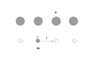
Figure 4: One-dimensional model of the lattice polaron on the chain interacting with displacements of all ions of another chain.

If the interaction is short-ranged, $g_{\alpha}({\bf m})=\kappa\delta_{{\bf m},0}$ (the Holstein model), then $g^{2}=E_{p}/\omega$. Here $\kappa$ is a constant. In general, we have $g^{2}=\gamma E_{p}/\omega$ with the numerical coefficient $\gamma$ less than $1$. To estimate $\gamma$ let us consider a one-dimensional chain model with the long-range Coulomb interaction between the electron on chain ($\times)$ and ion vibrations of another chain ($\circ),$ polarized in the direction perpendicular to the chains Korn2 , Fig.4. The corresponding force is given by

$$g_{\alpha}({\bf m-n})({\bf e}_{\alpha}\cdot{\bf u}_{{\bf m-n}})=\frac{\kappa}{(|{\bf m}-{\bf n}|^{2}+1)^{3/2}}.$$ (43)

Here the distance along the chains $|{\bf m}-{\bf n}|$ is measured in units of the lattice constant $a$, the inter-chain distance is also $a$, and we take $a=1$. For this long-range interaction we obtain $\gamma=0.39$. Hence the effective mass renormalization is much smaller than in the Holstein model, roughly as $m_{SFP}^{\ast}\propto(m_{SHP}^{\ast})^{1/2}$.

Not only does the small polaron mass strongly depend on the radius of the electron-phonon interaction, but also does the range of the applicability of the analytical $1/\lambda$ expansion theory. The theory appears almost exact in a wide region of parameters for the Fröhlich interaction. The exact polaron mass in a wide region of the adiabatic parameter $\omega/T(a)$ and coupling was calculated with the continuous-time path-integral Quantum Monte Carlo (QMC) algorithm Korn2 . This method is free from any systematic finite-size, finite-time-step and finite-temperature errors and allows for an exact (in the QMC sense) calculation of the ground-state energy and the effective mass of the lattice polaron for any electron-phonon interaction.

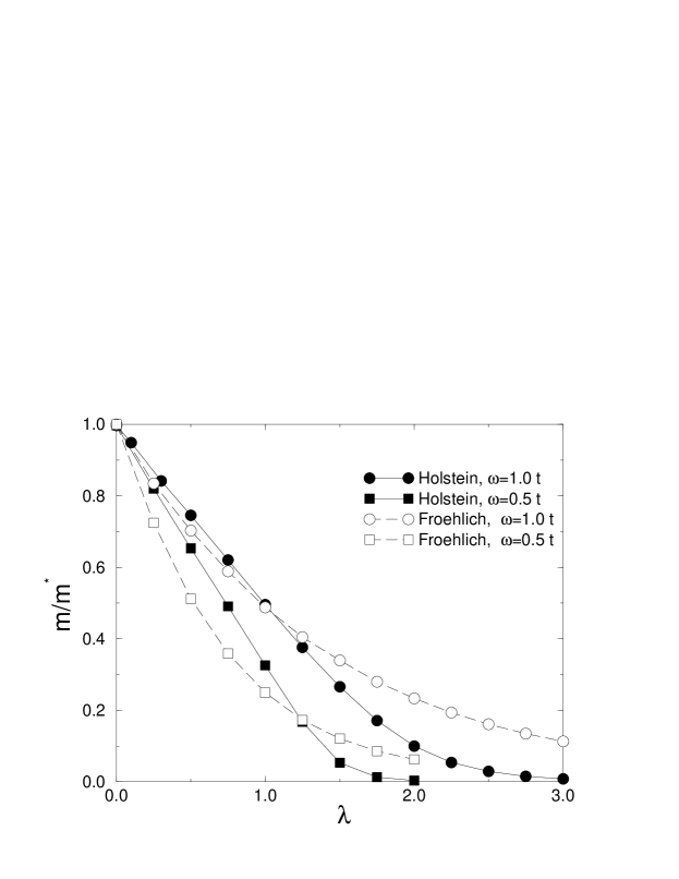
Figure 5: Inverse effective polaron mass in units of $1/m=2T(a)a^{2}$ ($T(a)=t$ on the graph) Korn2

At large $\lambda$ ($>1.5$) SFP was found to be much lighter than SHP, while the large Fröhlich polaron (i.e. at $\lambda<1$) was $heavier$ than the large Holstein polaron with the same binding energy, Fig.5. The mass ratio $m_{FP}^{\ast}/m_{HP}^{\ast}$ is a non-monotonic function of $\lambda$. The effective mass of the Fröhlich polaron, $m_{FP}^{\ast}(\lambda)$ is well fitted by a single exponent, which is $e^{0.73\lambda}$ for $\omega=T(a)$ and $e^{1.4\lambda}$ for $\omega=0.5\,T(a)$. The exponents are remarkably close to those obtained with the Lang-Firsov transformation, $e^{0.78\lambda}$ and $e^{1.56\lambda}$, respectively. Hence, in the case of the Fröhlich interaction the transformation is perfectly accurate even in the moderate adiabatic regime, $\omega/T(a)\leq 1$ for $any$ coupling strength. It is not the case for the Holstein polaron. If the interaction is short-ranged, the same analytical technique is applied only in the nonadiabatic regime $\omega/T(a)>1.$

Another interesting point is that the size of SFP and the length, over which the distortion spreads, are $different$. In the strong-coupling limit the polaron is almost localized on one site ${\bf m}$. Hence, the size of its wave function is the atomic size. On the other hand, the ion displacements, proportional to the displacement force $g_{\alpha}({\bf m-n})$, spread over a large distance. Their amplitude at a site ${\bf n}$ falls with the distance as $|{\bf m-n}|^{-3}$ in our one-dimensional model. The polaron cloud (i.e. lattice distortion) is more extended than the polaron itself. Such polaron tunnels with a larger probability than the Holstein polaron due to a smaller $relative$ lattice distortion around two neighboring sites. For the short-range e-ph interaction the entire lattice deformation disappears at one site and then forms at its neighbor, when the polaron tunnels from site to site. Therefore $\gamma=1$ and the polaron is very heavy already at $\lambda\approx 1$. On the contrary, if the interaction is long-ranged, only a fraction of the total deformation changes every time the polaron tunnels from one site to its neighbor, and $\gamma$ is smaller than $1.$ A lighter mass of SFP compared with the nondispersive SHP is a generic feature of any dispersive electron-phonon interaction.

II.6 Attractive correlations of small polarons

Lattice deformation also strongly affects the interaction between electrons. At large distances polarons repel each other in ionic crystals, but their Coulomb repulsion is substantially reduced due to ion polarization. Nevertheless two $large$ polarons can be bound into a $large$ bipolaron by an exchange interaction even with no additional e-ph interaction but the Fröhlich one vin ; sup ; ada ; emin ; bas ; ver0 .

When a short-range deformation potential and molecular e-ph interactions (e.g. of the Jahn-Teller type mul00 ) are taken into account together with the long-range Fröhlich interaction, they can overcome the Coulomb repulsion ale5 . The resulting interaction becomes attractive at a short distance of about a lattice constant. Then two small polarons readily form a bound state, i.e. a $small$ bipolaron ander ; cha ; alerun ; aubr , because their band is narrow. Consideration of particular lattice structures shows that small bipolarons are mobile even when the electron-phonon coupling is strong and the bipolaron binding energy is large ale5 (see below). Here we encounter a novel electronic state of matter, a charged Bose liquid of electron molecules with double elementary charge 2e, qualitatively different from normal Fermi-liquids in ordinary metals and from the Bardeen-Cooper-Schrieffer (BCS) superfluids in conventional superconductors.

The origin of the attractive force between two small polarons can be readily understood from about the same toy model as in Fig.2, but with two electrons on neighbor sites 1,2 interacting with an ion in between 3, Fig.6. For generality we now assume that the ion is a three-dimensional oscillator described by a displacement vector $\bf u$, rather than by a single-component displacement $x$ as in Fig.2.

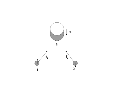
Figure 6: Two localized electrons shift the equilibrium position of the ion (${\bf 3}$). As a result two electrons on neighboring sites ${\bf 1}$ and ${\bf 2}$ attract each other.

The vibration part of the Hamiltonian in the model is

$$H_{ph}=-{1\over{2M}}\left({\partial\over{\partial{\bf u}}}\right)^{2}+{ku^{2}\over{2}},$$ (44)

Electron potential energies due to the Coulomb interaction with the ion are approximately

$$V_{1,2}=V_{0}(1-{\bf u}\cdot{\bf e_{1,2}}/a),$$ (45)

where ${\bf e_{1,2}}$ are units vectors connecting sites ${\bf 1,2}$ and site ${\bf 3}$, respectively. Hence the Hamiltonian of the model is given by

$$H=E_{a}(\hat{n}_{1}+\hat{n}_{2})+{\bf u}\cdot({\bf f_{1}}\hat{n}_{1}+{\bf f_{2}}\hat{n}_{2})-{1\over{2M}}\left({\partial\over{\partial{\bf u}}}\right)^{2}+{ku^{2}\over{2}},$$ (46)

where ${\bf f_{1,2}}=Ze^{2}{\bf e_{1,2}}/a^{2}$ is the Coulomb force, and $\hat{n}_{1,2}$ are occupation number operators at every site. This Hamiltonian is also readily diagonalized by the same displacement transformation of the vibronic coordinate ${\bf u}$ as above,

$${\bf u}={\bf v}-\left({\bf f_{1}}\hat{n}_{1}+{\bf f_{2}}\hat{n}_{2}\right)/k.$$ (47)

The transformed Hamiltonian has no electron-phonon coupling,

$$\tilde{H}=(E_{a}-E_{p})(\hat{n}_{1}+\hat{n}_{2})+V_{ph}\hat{n}_{1}\hat{n}_{2}-{1\over{2M}}\left({\partial\over{\partial{\bf v}}}\right)^{2}+{kv^{2}\over{2}},$$ (48)

and describes two small polarons at their atomic levels shifted by the polaron level shift $E_{p}=f_{1,2}^{2}/2k$, which are entirely decoupled from ion vibrations. As a result, the lattice deformation caused by two electrons leads to an effective interaction between them, $V_{ph}$, which should be added to their Coulomb repulsion, $V_{c}$,

$$V_{ph}=-{\bf f_{1}}\cdot{\bf f_{2}}/k.$$ (49)

When $V_{ph}$ is negative and larger by magnitude than the positive $V_{c}$ the resulting interaction becomes attractive.

Applying the polaron canonical transformation to a generic “Fröhlich-Coulomb” Hamiltonian, allows us explicitly calculate the effective attraction of small polarons alekor , Eq.(38), and elaborate more physics behind the lattice sums in Eq.(3,38) and Eq.(41). If a carrier (electron or hole) acts on an ion with a force ${\bf f}$, it displaces the ion by some vector ${\bf x}={\bf f}/k$. Here $k$ is the ion’s force constant. The total energy of the carrier-ion pair is $-{\bf f}^{2}/(2k)$. This is precisely the summand in Eq.(3) expressed via dimensionless coupling constants. Now consider two carriers interacting with the same ion, see Fig.7. The ion displacement is ${\bf x}=({\bf f}_{1}+{\bf f}_{2})/k$ and the energy is $-{\bf f}_{1}^{2}/(2k)-{\bf f}_{2}^{2}/(2k)-({\bf f}_{1}\cdot{\bf f}_{2})/k$. Here the last term should be interpreted as an ion-mediated interaction between the two carriers. It depends on the scalar product of ${\bf f}_{1}$ and ${\bf f}_{2}$ and consequently on the relative positions of the carriers with respect to the ion. If the ion is an isotropic harmonic oscillator, as we assume here, then the following simple rule applies. If the angle $\phi$ between ${\bf f}_{1}$ and ${\bf f}_{2}$ is less than $\pi/2$ the polaron-polaron interaction will be attractive, if otherwise it will be repulsive. In general, some ions will generate attraction, and some repulsion between polarons, Fig.7.

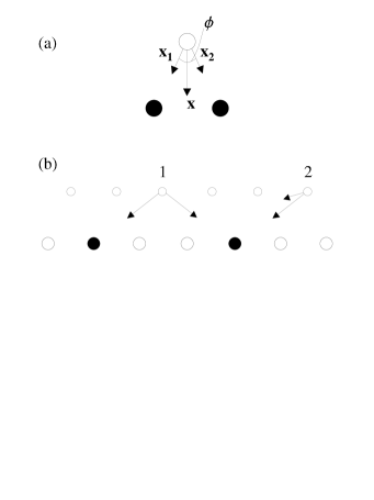
Figure 7: Mechanism of the polaron-polaron interaction. (a) Together, two polarons (solid circles) deform the lattice more effectively than separately. An effective attraction occurs when the angle $\phi$ is less than $\pi/2$ . (b) A mixed situation. Ion 1 results in repulsion between two polarons while ion 2 results in attraction.

The overall sign and magnitude of the interaction is given by the lattice sum in Eq.(38), the evaluation of which is elementary. One should also note that according to Eq.(41) an attractive interaction reduces the polaron mass (and consequently the bipolaron mass), while repulsive interaction enhances the mass.

III Superlight bipolarons in high-$T_{c}$ cuprates

Consideration of particular lattice structures shows that small inter-site bipolarons are perfectly mobile even when the electron-phonon coupling is strong and the bipolaron binding energy is large. Let us analyze the important case of copper-based high-$T_{c}$ oxides. As discussed in the introduction they are doped charged-transfer ionic insulators with narrow electron bands. Therefore, the interaction between holes can be analyzed using computer simulation techniques based on a minimization of the ground state energy of an ionic insulator with two holes, the lattice deformations and the Coulomb repulsion fully taken into account, but neglecting the kinetic energy terms. Using these techniques net inter-site interactions of the in-plane oxygen hole with the $apex$ hole, Fig.8, and of two in-plane oxygen holes, Fig.10, were found to be attractive in $La_{2}CuO_{4}$ cat with the binding energies $\Delta=119meV$ and $\Delta=60meV$, respectively. All other interactions were found to be repulsive.

III.1 Apex bipolarons

Both apex and in-plane bipolarons can tunnel from one unit cell to another via the  single-polaron tunnelling from one apex oxygen to its apex neighbor in case of the apex bipolaron ale5 , Fig.8, or via the next-neighbor hopping in case of the in-plane bipolaron alekor , Fig.10.

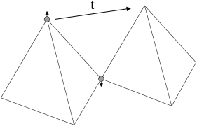
Figure 8: Apex bipolaron tunnelling in perovskites

The Bloch bands of these bipolarons are obtained using the canonical transformation, described above, projecting the transformed Hamiltonian, Eq.(37), onto a reduced Hilbert space containing only empty or doubly occupied elementary cells, and averaging the result with respect to phonons alebook1 . The wave function of the apex bipolaron localized, let us say, in the cell ${\bf m}$ is written as

$$|{\bf m}\rangle=\sum_{i=1}^{4}A_{i}c_{i}^{\dagger}c_{apex}^{\dagger}|0\rangle,$$ (50)

where $i$ denotes the $p_{x,y}$ orbitals and spins of the four plane oxygen ions in the cell, Fig.8 and $c_{apex}^{\dagger}$ is the creation operator for the hole on one of the three apex oxygen orbitals with the spin, which is the same or opposite of the spin of the in-plane hole depending on the total spin of the bipolaron. The probability amplitudes $A_{i}$ are normalized by the condition $|A_{i}|=1/2,$ if four plane orbitals $p_{x1},p_{y2},p_{x3}$ and $p_{y4}$ are involved, or by $|A_{i}|=1/\sqrt{2}$ if only two of them are relevant. Then a matrix element of the Hamiltonian Eq.(37) describing the bipolaron tunnelling to the nearest neighbor cell ${\bf m+a}$ is found as

$$t=\langle{\bf m}|\tilde{H}|{\bf m}+{\bf a}\rangle=|A_{i}|^{2}T_{pp^{\prime}}^{apex}e^{-g^{2}},$$ (51)

where $T_{pp^{\prime}}^{apex}e^{-g^{2}}$ is a single polaron hopping integral between two apex ions. The inter-site bipolaron tunnelling appears already in the first order with respect to the single-hole transfer $T_{pp^{\prime}}^{apex}$, and the bipolaron energy spectrum consists of two bands $E^{x,y}({\bf K),}$ formed by the overlap of $p_{x}$ and $p_{y}$ $apex$ oxygen orbitals, respectively:

$$E^{x}({\bf K}) = t\cos(K_{x})-t^{\prime}\cos(K_{y}),$$ (52)

$$E^{y}({\bf K}) = -t^{\prime}\cos(K_{x})+t\cos(K_{y}).$$

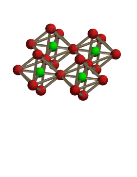
Figure 9: Simplified model of the copper-oxygen perovskite layer.

They transform into one another under $\pi/2$ rotation. If $t,t^{\prime}>0,$ “$x"$ bipolaron band has its minima at ${\bf K=}(\pm\pi,0)$ and $y$-band at ${\bf K}=(0,\pm\pi)$. In these equations $t$ is the renormalized hopping integral between $p$ orbitals of the same symmetry elongated in the direction of the hopping ($pp\sigma$) and $t^{\prime}$ is the renormalized hopping integral in the perpendicular direction ($pp\pi$). Their ratio $t/t^{\prime}=T_{pp^{\prime}}^{apex}/T^{\prime}{}_{pp^{\prime}}^{apex}=4$ as follows from the tables of hopping integrals in solids. Two different bands are not mixed because $T_{p_{x},p_{y}^{\prime}}^{apex}=0$ for the nearest neighbors. A random potential does not mix them either, if it varies smoothly on the lattice scale. Hence, we can distinguish ‘$x$’ and ‘$y$’ bipolarons with a lighter effective mass in $x$ or $y$ direction, respectively. The apex $z$ bipolaron, if formed, is $ca.$ four times less mobile than $x$ and $y$ bipolarons. The bipolaron bandwidth is of the same order as the polaron one, which is a specific feature of inter-site bipolarons. For a large part of the Brillouin zone near $(0,\pi)$ for ‘$x$’ and $(\pi,0)$ for ‘$y$’ bipolarons, one can adopt the effective mass approximation

$$E^{x,y}({\bf K})={\frac{K_{x}^{2}}{{2m_{x,y}^{\ast\ast}}}}+{\frac{K_{y}^{2}}{{2m_{y,x}^{\ast\ast}}}}$$ (53)

with $K_{x,y}$ taken relative to the band bottom positions and $m_{x}^{\ast\ast}=1/t$, $m_{y}^{\ast\ast}=4m_{x}^{\ast\ast}$.

III.2 In-plane bipolarons

Now let us consider in-plane bipolarons in a two-dimensional lattice of ideal octahedra that can be regarded as a simplified model of the copper-oxygen perovskite layer, Fig.9 alekor . The lattice period is $a=1$ and the distance between the apical sites and the central plane is $h=a/2=0.5$. For mathematical transparency we assume that all in-plane atoms, both copper and oxygen, are static but apex oxygens are independent three-dimensional isotropic harmonic oscillators. Due to poor screening, the hole-apex interaction is purely coulombic,

$$g_{\alpha}({\bf m-n})=\frac{\kappa_{\alpha}}{|{\bf m-n}|^{2}},$$

where $\alpha=x,y,z$. To account for the experimental fact that $z$-polarized phonons couple to the holes stronger than others tim , we choose $\kappa_{x}=\kappa_{y}=\kappa_{z}/\sqrt{2}$. The direct hole-hole repulsion is

$$V_{c}({\bf n-n^{\prime}})=\frac{V_{c}}{\sqrt{2}|{\bf n-n^{\prime}}|}$$

so that the repulsion between two holes in the nearest neighbor (NN) configuration is $V_{c}$. We also include the bare NN hopping $T_{NN}$, the next nearest neighbor (NNN) hopping across copper $T_{NNN}$ and the NNN hopping between the pyramids $T_{NNN}^{\prime}$.

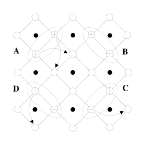
Figure 10: Four degenerate in-plane bipolaron configurations A, B, C, and D . Some single-polaron hoppings are indicated by arrows.

The polaron shift is given by the lattice sum Eq.(3), which after summation over polarizations yields

$$E_{p}=2\kappa_{x}^{2}\omega_{0}\sum_{{\bf m}}\left(\frac{1}{|{\bf m-n}|^{4}}+\frac{h^{2}}{|{\bf m-n}|^{6}}\right)=31.15\kappa_{x}^{2}\omega_{0},$$ (54)

where the factor $2$ accounts for two layers of apical sites. For reference, the Cartesian coordinates are ${\bf n}=(n_{x}+1/2,n_{y}+1/2,0)$, ${\bf m}=(m_{x},m_{y},h)$, and $n_{x},n_{y},m_{x},m_{y}$ are integers. The polaron-polaron attraction is

$$V_{ph}({\bf n-n^{\prime}})=4\omega\kappa_{x}^{2}\sum_{{\bf m}}\frac{h^{2}+({\bf m-n^{\prime}})\cdot({\bf m-n})}{|{\bf m-n^{\prime}}|^{3}|{\bf m-n}|^{3}}.$$ (55)

Performing the lattice summations for the NN, NNN, and NNN’ configurations one finds $V_{ph}=1.23\,E_{p},$ $0.80\,E_{p}$, and $0.82\,E_{p}$, respectively. As a result, we obtain a net inter-polaron interaction as $v_{NN}=V_{c}-1.23\,E_{p}$, $v_{NNN}=\frac{V_{c}}{\sqrt{2}}-0.80\,E_{p}$, $v_{NNN}^{\prime}=\frac{V_{c}}{\sqrt{2}}-0.82\,E_{p}$, and the mass renormalization exponents as $g_{NN}^{2}=0.38(E_{p}/\omega)$, $g_{NNN}^{2}=0.60(E_{p}/\omega)$ and $(g^{\prime}{}_{NNN})^{2}=0.59(E_{p}/\omega)$.

Let us now discuss different regimes of the model. At $V_{c}>1.23\,E_{p}$, no bipolarons are formed and the system is a polaronic Fermi liquid. Polarons tunnel in the square lattice with $t=T_{NN}\exp(-0.38E_{p}/\omega)$ and $t^{\prime}=T_{NNN}\exp(-0.60E_{p}/\omega)$ for NN and NNN hoppings, respectively. Since $g_{NNN}^{2}\approx(g_{NNN}^{\prime})^{2}$ one can neglect the difference between NNN hoppings within and between the octahedra. A single polaron spectrum is therefore

$$E_{1}({\bf k})=-E_{p}-2t^{\prime}[\cos k_{x}+\cos k_{y}]-4t\cos(k_{x}/2)\cos(k_{y}/2).$$ (56)

The polaron mass is $m^{\ast}=1/(t+2t^{\prime})$. Since in general $t>t^{\prime}$, the mass is mostly determined by the NN hopping amplitude $t$.

If $V_{c}<1.23\,E_{p}$ then intersite NN bipolarons form. The bipolarons tunnel in the plane via four resonating (degenerate) configurations $A$, $B$, $C$, and $D$, as shown in Fig.10. In the first order of the renormalized hopping integral, one should retain only these lowest energy configurations and discard all the processes that involve configurations with higher energies. The result of such a projection is the bipolaron Hamiltonian

$$H_{b} = (V_{c}-3.23\,E_{p})\sum_{{\bf l}}[A_{{\bf l}}^{\dagger}A_{{\bf l}}+B_{{\bf l}}^{\dagger}B_{{\bf l}}+C_{{\bf l}}^{\dagger}C_{{\bf l}}+D_{{\bf l}}^{\dagger}D_{{\bf l}}]$$

$$-t^{\prime}\sum_{{\bf l}}[A_{{\bf l}}^{\dagger}B_{{\bf l}}+B_{{\bf l}}^{\dagger}C_{{\bf l}}+C_{{\bf l}}^{\dagger}D_{{\bf l}}+D_{{\bf l}}^{\dagger}A_{{\bf l}}+H.c.]$$

$$-t^{\prime}\sum_{{\bf n}}[A_{{\bf l-x}}^{\dagger}B_{{\bf l}}+B_{{\bf l+y}}^{\dagger}C_{{\bf l}}+C_{{\bf l+x}}^{\dagger}D_{{\bf l}}+D_{{\bf l-y}}^{\dagger}A_{{\bf l}}+H.c.],$$

where ${\bf l}$ numbers octahedra rather than individual sites, ${\bf x}=(1,0)$, and ${\bf y}=(0,1)$. A Fourier transformation and diagonalization of a $4\times 4$ matrix yields the bipolaron spectrum:

$$E_{2}({\bf K})=V_{c}-3.23E_{p}\pm 2t^{\prime}[\cos(K_{x}/2)\pm\cos(K_{y}/2)].$$ (58)

There are four bipolaronic subbands combined in the band of the width $8t^{\prime}$. The effective mass of the lowest band is $m^{\ast\ast}=2/t^{\prime}$. The bipolaron binding energy is $\Delta\approx 1.23E_{p}-V_{c}.$ Inter-site bipolarons already move in the first order of the single polaron hopping. This remarkable property is entirely due to the strong on-site repulsion and long-range electron-phonon interactions that leads to a non-trivial connectivity of the lattice. This fact combines with a weak renormalization of $t^{\prime}$ yielding a superlight bipolaron with the mass $m^{\ast\ast}\propto\exp(0.60\,E_{p}/\omega)$. We recall that in the Holstein model $m^{\ast\ast}\propto\exp(2E_{p}/\omega)$ alerun . Thus the mass of the Fröhlich bipolaron in the perovskite layer scales approximately as a cubic root of that of the Holstein bipolaron.

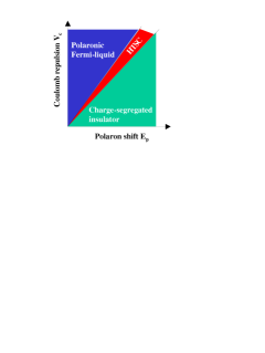
Figure 11: FCM phase diagram.

At even stronger e-ph interaction, $V_{c}<1.16E_{p}$, NNN bipolarons become stable. More importantly, holes can now form 3- and 4-particle clusters. The dominance of the potential energy over kinetic in the transformed Hamiltonian enables us to readily investigate these many-polaron cases. Three holes placed within one oxygen square have four degenerate states with the energy $2(V_{c}-1.23E_{p})+V_{c}/\sqrt{2}-0.80E_{p}$. The first-order polaron hopping processes mix the states resulting in a ground state linear combination with the energy $E_{3}=2.71V_{c}-3.26E_{p}-\sqrt{4t^{2}+t^{\prime}{}^{2}}$. It is essential that between the squares such triads could move only in higher orders of polaron hopping. In the first order, they are immobile. A cluster of four holes has only one state within a square of oxygen atoms. Its energy is $E_{4}=4(V_{c}-1.23E_{p})+2(V_{c}/\sqrt{2}-0.80E_{p})=5.41V_{c}-6.52E_{p}$. This cluster, as well as all bigger ones, are also immobile in the first order of polaron hopping. We would like to stress that at distances much larger than the lattice constant the polaron-polaron interaction is always repulsive, and the formation of infinite clusters, stripes or strings is prohibited. We conclude that at $V_{c}<1.16E_{p}$ the system quickly becomes a charge segregated insulator, Fig.11.

The fact that within the window, $1.16E_{p}<V_{c}<1.23E_{p}$, there are no three or more polaron bound states, means that bipolarons repel each other. The system is effectively a charged Bose-gas, which is a superconductor. The superconductivity window, that we have found, is quite narrow. This indicates that the superconducting state in cuprates requires a rather fine balance between electronic and ionic interactions, Fig.11.

III.3 Low-energy (bi)polaron energy structure of cuprates

The considerations set out above lead us to a simple model of cuprates alemot3 ; alebook1 . The main assumption is that $all$ $electrons$ are bound into small singlet and triplet $intersite$ bipolarons stabilized by e-ph interactions. As the undoped plane has a half-filled $Cu3d^{9}$ band there are no empty states for bipolarons to move if they are inter-site. Their Brillouin zone is half of the original electron BZ and is completely filled with hard-core bosons. $Hole$ pairs, which appear with doping, have enough empty states to move, and they are responsible for low-energy kinetics. Above $T_{c}$ a material such as $YBa_{2}Cu_{3}O_{6+x}$ contains a non-degenerate gas of hole bipolarons in singlet and in triplet states. Triplets are separated from singlets by a spin gap $J$ and have a lower mass due to a lower binding energy, Fig.12. The main part of the electron-electron correlation energy (Hubbard $U$ and the inter-site Coulomb repulsion) and the electron-phonon interaction are taken into account in the binding energy of bipolarons $\Delta,$ and in their band-width renormalization as described above. When the hole density is small, $n_{b}\ll 1$ (as in cuprates), their bipolaronic operators are almost bosonic. The hard-core interaction does not play any role in this dilute limit, so only the long-distance Coulomb repulsion is relevant. This repulsion is significantly reduced due to a large static dielectric constant in oxides, $\epsilon_{0}\gg 1$. Hence, carriers are almost free charged bosons coexisting with thermally excited nondegenerate single fermions, so that the conventional Boltzmann kinetics (see below) and the Bogoliubov transformation bog for a charged Bose gas are perfectly applied in the normal and in the superconducting state, respectively.

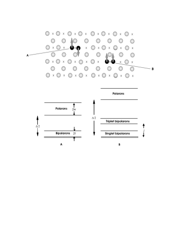
Figure 12: Bipolaron picture of high temperature superconductors. $A$ corresponds to a singlet intersite bipolaron. $B$ is a triplet intersite bipolaron, which naturally includes the addition of an extra excitation band. The crosses are copper sites and the circles are oxygen sites, $w$ is a half bandwidth of the polaron band, $t$ is a half bandwidth of the bipolaronic band, $\Delta/2$ is the bipolaron binding energy per polaron and $J$ is the exchange energy per bipolaron.

The population of singlet, $n_{s}$, triplet $n_{t}$, and polaron, $n_{p}$ bands is determined by the chemical potential $\mu\equiv T\ln y$, where $y$ is found using the thermal equilibrium of singlet and triplet bipolarons and polarons,

$$2n_{s}+2n_{t}+n_{p}=x.$$ (59)

Applying the effective-mass approximation for quasi-two-dimensional energy spectra of all particles we obtain for $0<y<1$

$$-m_{s}^{\ast\ast}\ln\left({1-y}\right)-3m_{t}^{\ast\ast}\ln\left({1-ye^{-J/T}}\right)+m^{\ast}\ln\left({1+y}^{1/2}{e^{-\Delta/(2T)}}\right)={\frac{\pi x}{{T}}},$$ (60)

in the normal state, and $y=1$ in the superconducting state. Here $x$ is the total number of holes per unit area. If the polaron energy spectrum is (quasi)one-dimensional, an additional $T^{-1/2}$ appears in front of $\ln$ in the third term on the left hand side of Eq.(59).

III.4 Role of disorder and the phase diagram of cuprates

We should also take into account localization of holes by the random potential, because doping inevitably introduces some disorder. The Coulomb repulsion restricts the number of charged bosons in each localized state, so that the distribution function will show a mobility edge $E_{c}$ alebramot . The number of bosons in a single potential well is determined by the competition between their long-range Coulomb repulsion c.a. ${4e^{2}/(\epsilon_{0}\xi)}$ and the binding energy $E_{c}-\epsilon$. If the localization length diverges with the critical exponent $\nu<1$ $(\xi\sim{(E_{c}-\epsilon)^{-\nu}})$, we can apply a ‘single well-single particle’ approximation assuming that there is only one boson in each potential well. Within this approximation $localized$ $charged$ bosons effectively obey the Fermi-Dirac statistics, so that their density is given by

$$n_{L}(T)=\int_{-\infty}^{E_{c}}{\frac{N_{L}(E)dE}{y^{-1}{\exp(E/T)+1}}},$$ (61)

where $N_{L}(E)$ is the density of localized states. Near the mobility edge it remains constant $N_{L}(E)\approx{n_{L}/\Gamma,}$ where ${\Gamma}$ is of the order of the binding energy in a single random potential well, and $n_{L}$ is the number of localized states per unit area. The number of $empty$ localized states turns out to be linear as a function of temperature in a wide temperature range $T<\Gamma$ from Eq.(60). Then the conservation of the total number of carriers yields for the chemical potential:

$$\frac{\pi(x-2n_{L})}{T} = -m_{s}^{\ast\ast}\ln\left({1-y}\right)-3m_{t}^{\ast\ast}\ln\left({1-ye^{-J/T}}\right)+$$

$$m^{\ast}\ln\left({1+y}^{1/2}{e^{-\Delta/(2T)}}\right)-{\frac{2\pi n_{L}}{{\Gamma}}}\ln(1+y^{-1}).$$

If the number of localized states is about the same as the number of pairs, $n_{L}\approx x/2$, a solution of this equation does not depend on temperature in a wide temperature range above $T_{c}$. With $y$ to be a constant ($y\approx 0.6$ in a wide range of parameters in Eq.(61)), the number of singlet bipolarons in the Bloch states is linear in temperature,

$$n_{s}(T)=(x/2-n_{L})+T{\frac{n_{L}}{{\Gamma}}}\ln(1+y^{-1}).$$ (63)

The numbers of triplet pairs and single polarons are exponentially small at low temperatures, $T\ll J,\Delta/2.$

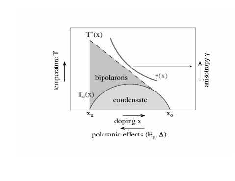
Figure 13: Phase diagram of superconducting cuprates in the bipolaron theory (courtesy of J. Hofer).

The model suggests a phase diagram of the cuprates as shown in Fig.13. This phase diagram is based on the assumption that to account for the high values of $T_{c}$ in cuprates one has to consider electron-phonon interactions larger than those used in the BSC-Eliashberg theory of superconductivity. Regardless of the adiabatic ratio, the Migdal-Eliashberg theory of superconductivity and the Fermi-liquid theory break at $\lambda\approx 1$. The many-electron system collapses into the small (bi)polaron regime at $\lambda\geq 1$ with well separated vibrational and charge-carrier degrees of freedom. Even though it seems that these carriers should have a mass too large to be mobile, the inclusion of the on-site Coulomb repulsion and a poor screening of the long-range electron-phonon interaction leads to $mobile$ intersite bipolarons as discussed above. In the normal state the Bose gas of the bipolarons is non-degenerate and below $T_{c}$ their phase coherence sets in and hence superfluidity of the double-charged $2e$ bosons occurs. There are also thermally excited single polarons and triplets in the model, Fig.12, which are responsible for the crossover regime at $T^{\ast}$ and normal state charge and spin (pseudo)gaps in cuprates. These pseudogaps were predicted as half of the binding energy $\Delta$ and the singlet-triplet exchange energy $J$ of preformed bipolarons, respectively alegap . $T^{\ast}$ is a temperature, where the polaron density compares with the bipolaron one.

III.5 Low Fermi energy: individual pairing in cuprates

Clear evidence for bipolarons comes from a parameter-free estimate alefermi of the renormalized Fermi-energy $\epsilon_{F}$, which yields a very small value in cuprates, where the band structure is quasi-two-dimensional with a few degenerate hole pockets. Applying the parabolic approximation for the band dispersion we obtain the renormalized Fermi energy as

$$\epsilon_{F}={\frac{\pi n_{i}d}{{m_{i}^{\ast}}}},$$ (64)

where $d$ is the interplane distance, and $n_{i},m_{i}^{\ast}$ are the density of holes and their effective mass in each of the hole subbands $i$ renormalized by the electron-phonon interaction. One can express the renormalized band-structure parameters through the in-plane magnetic-field penetration depth at $T\approx 0$, measured experimentally:

$$\lambda_{H}^{-2}=4\pi e^{2}\sum_{i}\frac{n_{i}}{m_{i}^{\ast}}.$$ (65)

As a result, we obtain a parameter-free expression for the “true” (i.e. renormalized) Fermi energy as

$$\epsilon_{F}={\frac{d}{{4ge^{2}\lambda_{H}^{2}}}},$$ (66)

where $g$ is the degeneracy of the spectrum, which may depend on doping in cuprates. One expects $4$ hole pockets inside BZ due to the Mott-Hubbard gap in underdoped cuprates. If the hole band minima are shifted with doping to BZ boundaries, all their wave vectors would belong to the stars with two or more prongs. The groups of wave vectors for these stars have only 1D representations. It means that the spectrum will be degenerate with respect to the number of prongs which the star has, i.e $g\geq 2$. The only exception is the minimum at ${\bf k}=(\pi,\pi)$ with one prong and $g=1$. Hence, in cuprates the degeneracy is $1\leq g\leq 4$. Because Eq.(65) does not contain any other band-structure parameters, the estimate of $\epsilon_{F}$ using this equation does not depend very much on the parabolic approximation for the band dispersion.

Generally, the ratios $n/m^{\ast}$ in Eq.(63) and in Eq.(64) are not necessarily the same. The ‘superfluid’ density in Eq.(64) might be different from the total density of delocalized carriers in Eq.(63). However, in a translation invariant system they must be the same pop . This is also true even in the extreme case of a pure two-dimensional superfluid, where quantum fluctuations are important. One can, however, obtain a reduced value of the zero temperature superfluid density in the dirty limit, $l\ll\xi(0)$, where $\xi(0)$ is the zero-temperature coherence length. The latter was measured directly in cuprates as the size of the vortex core. It is about 10 $\AA$ or even less. On the contrary, the mean free path was found surprisingly large at low temperatures, $l\sim$ 100-1000 $\AA$. Hence, it is rather probable that all cuprate superconductors are in the clean limit, $l\gg\xi(0)$, so the parameter-free expression for $\epsilon_{F}$, Eq.(65), is perfectly applicable.

Table 1: The Fermi energy (multiplied by the degeneracy) of cuprates

Compound	$T_{c}$ (K)	$\lambda_{H,ab}$ $(\AA)$	d$(\AA)$	$g\epsilon_{F}$ (meV)
$La_{1.8}Sr_{0.2}CuO_{4}$	36.2	2000	6.6	112
$La_{1.78}Sr_{0.22}CuO_{4}$	27.5	1980	6.6	114
$La_{1.76}Sr_{0.24}CuO_{4}$	20.0	2050	6.6	106
$La_{1.85}Sr_{0.15}CuO_{4}$	37.0	2400	6.6	77
$La_{1.9}Sr_{0.1}CuO_{4}$	30.0	3200	6.6	44
$La_{1.75}Sr_{0.25}CuO_{4}$	24.0	2800	6.6	57
$YBa_{2}Cu_{3}O_{7}$	92.5	1400	4.29	148
$YBa_{2}Cu_{3}O_{6.7}$	66.0	2100	4.29	66
$YBa_{2}Cu_{3}O_{6.57}$	56.0	2900	4.29	34
$YBa_{2}Cu_{3}O_{6.92}$	91.5	1861	4.29	84
$YBa_{2}Cu_{3}O_{6.88}$	87.9	1864	4.29	84
$YBa_{2}Cu_{3}O_{6.84}$	83.7	1771	4.29	92
$YBa_{2}Cu_{3}O_{6.79}$	73.4	2156	4.29	62
$YBa_{2}Cu_{3}O_{6.77}$	67.9	2150	4.29	63
$YBa_{2}Cu_{3}O_{6.74}$	63.8	2022	4.29	71
$YBa_{2}Cu_{3}O_{6.7}$	60.0	2096	4.29	66
$YBa_{2}Cu_{3}O_{6.65}$	58.0	2035	4.29	70
$YBa_{2}Cu_{3}O_{6.6}$	56.0	2285	4.29	56
$HgBa_{2}CuO_{4.049}$	70.0	2160	9.5	138
$HgBa_{2}CuO_{4.055}$	78.2	1610	9.5	248
$HgBa_{2}CuO_{4.055}$	78.5	2000	9.5	161
$HgBa_{2}CuO_{4.066}$	88.5	1530	9.5	274

A parameter-free estimate of the Fermi energy obtained by using Eq.(65) is presented in Table 1. The renormalized Fermi energy in many cuprates is less than $100$ $meV$, if the degeneracy $g\geq 2$ is taken into account. That should be compared with the characteristic phonon frequency, which is estimated as the plasma frequency of oxygen ions,

$$\omega=\sqrt{\frac{4\pi Z^{2}e^{2}N}{M}}.$$ (67)

One obtains $\omega$=$84meV$ with $Z=2$, $N=6/V_{cell}$, $M=16a.u.$ for $YBa_{2}Cu_{3}O_{6}$. Here $V_{cell}$ is the volume of the (chemical) unit cell. The estimate agrees with the measured phonon spectra. As established experimentally in cuprates (see the introduction) high-frequency optical phonons are strongly coupled with holes. A low Fermi energy is a serious problem for the Migdal-Eliashberg approach. Since the Fermi energy is small and phonon frequencies are high, the Coulomb pseudopotential $\mu_{c}^{\ast}$ is of the order of the bare Coulomb repulsion, $\mu_{c}^{\ast}\simeq\mu_{c}\simeq 1$ since the Tolmachev-Morel-Anderson logarithm is ineffective. Hence, to get a pairing, one has to have a strong coupling, $\lambda>\mu_{c}$. However, one cannot increase $\lambda$ without accounting for the polaron collapse of the band. Even in the region of the applicability of the BCS-Eliashberg theory (i.e. at $\lambda\leq 0.5$), the non-crossing diagrams cannot be treated as vertex $corrections$ like in Ref.pie , since they are comparable to the standard terms, when $\omega/\epsilon_{F}\geq 1$.

In many cases (Table 1) the renormalized Fermi energy is so small that pairing is certainly individual, i.e. the bipolaron size is smaller than the inter-carrier distance. Indeed, this is the case, if

$$\epsilon_{F}\leq\pi\Delta.$$ (68)

If the bipolaron binding energy is twice of the pseudogap experimentally measured in the normal state of many cuprates kabmic , $\Delta>100meV,$ Eq.(67) is well satisfied in underdoped and even in a few optimally and overdoped cuprates. One should notice that the coherence length in a charged Bose gas has nothing to do with the size of the boson. It depends on the interparticle distance and the mean-free path alebook1 , and might be as large as in the BCS superconductor. Hence, it would be incorrect to apply the ratio of the coherence length to the inter-carrier distance as a criterium of the BCS-Bose liquid crossover. The correct criterium is given by Eq.(67).

IV Normal state properties of cuprates in FCM

The low-energy FCM electronic structure of cuprates is shown in Fig.12 alemot3 . Polaronic p-holes are bound in lattice inter-site singlets (A) or in singlets and triplets (B) (if spins are included in Eq.(2)) at any temperature. Above T_c a charged bipolaronic Bose liquid is non-degenerate and below $T_{c}$ phase coherence (ODLRO) of the preformed bosons sets in. The state above $T_{c}$ is perfectly ”normal” in the sense that the off-diagonal order parameter (i.e. the Bogoliubov-Gor’kov anomalous average $\cal{F}(\mathbf{r,r^{\prime}})=\langle\psi_{\downarrow}(\mathbf{{r})\psi_{\uparrow}({r^{\prime}}\rangle}$) is zero above the resistive transition temperature $T_{c}$. Here $\psi_{\downarrow,\uparrow}(\mathbf{r})$ annihilates electrons with spin $\downarrow,\uparrow$ at point ${\bf r}$. (Bi)polarons and thermally excited phonons are well decoupled in the strong-coupling regime of the electron-phonon interaction, so the conventional Boltzmann kinetics for mobile polaronic and bipolaronic carries is applied.

IV.1 Normal state in-plane resistivity, the Hall effect, magnetic susceptibility and the Lorenz number

A nonlinear temperature dependence of the $in$-plane resistivity below $T^{\ast}$, a temperature-dependent paramagnetic susceptibility, and a peculiar maximum in the Hall ratio well above $T_{c}$ have remained long-standing problems of cuprate physics. The bipolaron model provides their quantitative description alebramot ; jung ; alezavdzu . Here we use a ‘minimum’ bipolaron model Fig.12A, which includes the singlet bipolaron band and the spin 1/2 polaron band separated by $T^{\ast}$, and the $\tau-$approximation in weak electric ${\bf E}$ and magnetic fields, $\bf B\perp E$ alezavdzu . Bipolaron and single-polaron non-equilibrium distributions are found as

$$f({\bf k})=f_{0}(E)+\tau\frac{\partial f_{0}}{\partial E}{\bf v}\cdot\left\{{\bf F}+\Theta{\bf n}\times{\bf F}\right\},$$ (69)

where ${\bf v=}\partial E/\partial{\bf k,}$ ${\bf F}={\vec{\bf\nabla}}(\mu-2e\phi)$, $f_{0}(E)=[y^{-1}{\exp(E/T)-1]}^{-1}$ and the Hall angle $\Theta=\Theta_{b}=2eB\tau_{b}/m_{b}$ for bipolarons with the energy $E=k^{2}/(2m_{b})$, and ${\bf F}={\vec{\bf\nabla}}(\mu/2-e\phi)$, $f_{0}(E)=\{y^{-1/2}{\exp[(E+T^{\ast})/T]+1\}}^{-1}$, $E=k^{2}/(2m_{p})$, and $\Theta=\Theta_{p}=eB\tau_{p}/m_{p}$ for thermally excited polarons. Here $m_{b}$ and $m_{p}$ are the bipolaron and polaron mass, respectively, $y=\exp(\mu/T),$ $\mu$ is the chemical potential, and ${\bf n=B/}B$ is a unit vector in the direction of the magnetic field. Eq.(68) is used to calculate the electrical resistivity and the Hall ratio as

$$\rho = \frac{m_{b}}{4e^{2}\tau_{b}n_{b}(1+An_{p}/n_{b})},$$ (70)

$$R_{H} = \frac{1+2A^{2}n_{p}/n_{b}}{2en_{b}(1+An_{p}/n_{b})^{2}},$$ (71)

where $A=\tau_{p}m_{b}/(4\tau_{b}m_{p})$. The atomic densities of quasi two-dimensional carriers are found as

$$n_{b}=\frac{m_{b}T}{2\pi}|\ln(1-y)|,$$ (72)

$$n_{p}=\frac{m_{p}T}{\pi}\ln\left[1+y^{1/2}\exp\left(-T^{\ast}/T\right)\right].$$ (73)

and the chemical potential is determined by doping $x$ using $2n_{b}+n_{p}=x-n_{L}$, where $n_{L}$ is the number of carriers localized by disorder (here we take the lattice constant $a=1$).

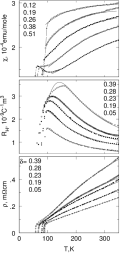
Figure 14: Uniform magnetic susceptibility, $\chi(T)$, Hall ratio, $R_{H}(T)$ and resistivity, $\rho(T)$, of underdoped $YBa_{2}Cu_{3}O_{7-\delta}$ coop fitted by the theory; see the Table below for parameters.

Polarons are not degenerate. Their number remains small compared with twice the number of bipolarons, $n_{p}/(2n_{b})<0.2$, in the relevant temperature range $T<T^{\ast}$, so that

$$y\approx 1-\exp(-T_{0}/T),$$ (74)

where $T_{0}=\pi(x-n_{L})/m_{b}\approx T_{c}$ is about the superconducting critical temperature of the (quasi)two-dimensional Bose gas. Because of this reason, the experimental $T_{c}$ was taken as $T_{0}$ in our fits. Using Eqs.(70,71,72) we obtain

$$R_{H}(T)=R_{H0}\frac{1+2A^{2}y^{1/2}(T/T_{c})\exp\left(-T^{\ast}/T\right)}{[1+A(T/T_{c})y^{1/2}\exp\left(-T^{\ast}/T\right)]^{2}},$$ (75)

where $R_{H0}=[e(x-n_{L})]^{-1}$. If we assume that the number of localized carriers depends only weakly on temperature in underdoped cuprates since their average ionization energy is sufficiently large, then $R_{H0}$ is temperature independent at $T<T^{\ast}$. As proposed in Ref.alebramot the scattering rate at relatively high temperatures is due to inelastic collisions of itinerant carriers with those localized by disorder, so it is proportional to $T^{2}$. We also have to take into account the residual scattering of polarons by optical phonons, so that $\tau^{-1}\propto(T/T_{1})^{2}+\exp\left(-\omega/T\right)$, if the temperature is low compared with the characteristic phonon energy $\omega$. The relaxation times of each type of carriers scales with their charge $e^{\ast}$ and mass as $\tau_{p,b}\propto m_{p,b}^{-3/2}(e^{\ast})^{-2}$, so we estimate $A=(m_{b}/m_{p})^{5/2}\approx 6$ if we take $m_{b}\approx 2m_{p}$ . As a result the in-plane resistivity is given by

$$\rho(T)=\rho_{0}\frac{(T/T_{1})^{2}+\exp\left(-\omega/T\right)}{[1+A(T/T_{c})y^{1/2}\exp\left(-T^{\ast}/T\right)]},$$ (76)

where $\rho_{0}\sim m_{b}/[2e^{2}(x-n_{L})]$ and $T_{1}$ are temperature independent. Finally, one can easily obtain the uniform magnetic susceptibility due to nondegenerate spin 1/2 polarons as AKM

$$\chi(T)=By^{1/2}\exp\left(-T^{\ast}/T\right)+\chi_{0},$$ (77)

where $B=(\mu_{B}^{2}m_{p}/\pi)$, and $\chi_{0}$ is the magnetic susceptibility of the parent Mott insulator.

$\delta$	$T_{c}$	$\rho_{0}$	$R_{H0}$	$10^{4}B$	$10^{4}\chi_{0}$	$T^{*}$	$\omega$	$T_{1}$
	K	$m\Omega cm$	$\frac{10^{-9}m^{3}}{C}$	$\frac{emu}{mole}$	$\frac{emu}{mole}$	K	K	K
0.05	90.7	1.8	0.45			144	447	332
0.12	93.7			2.6	2.1	155
0.19	87	3.4	0.63	4.5	1.6	180	477	454
0.23	80.6	5.7	0.74			210	525	586
0.26	78			5.4	1.5	259
0.28	68.6	8.9	0.81			259	594	786
0.38	61.9			7.2	1.4	348
0.39	58.1	17.8	0.96			344	747	1088
0.51	55			9.1	1.3	494

Our model numerically fits the Hall ratio, $R_{H}(T)$, the in-plane resistivity, $\rho(T)$, and the magnetic susceptibility $\chi(T)$ of $YBa_{2}Cu_{3}O_{7-\delta}$ within the physically relevant range of all parameters (see Fig.14 and the Table). The ratio of polaron and bipolaron mobilities $A=7$ used in all fits is close to the above estimate, and $\chi_{0}\approx 1.5\times 10^{-4}emu/mole$ is very close to the susceptibility of a slightly doped insulator coop . The maximum of $R_{H}(T)$ is due to the contribution of thermally excited polarons into transport, and the temperature dependence of the in-plane resistivity below $T^{\ast}$ is due to this contribution and the combination of the carrier-carrier and carrier-phonon scattering. The characteristic phonon frequency from the resistivity fit (see the Table) decreases with doping and the pseudogap $T^{\ast}$ shows the doping behavior as observed in other independent experiments kabmic .

Notwithstanding our explanation of the Hall ratio, the in-plane resistivity and the bulk magnetic susceptibility might be not so convincing as a direct measurement of the double charge $2e$ on carriers in the normal state. In 1993, we discussed the thermal conductivity of preformed bosons NEV . The contribution from carriers to the thermal transport provided by the Wiedemann-Franz law depends strongly on the elementary charge as $\sim(e^{\ast})^{-2}$ and should be significantly suppressed if $e^{\ast}=2e$. The Lorenz number, $L$, has been directly measured in $YBa_{2}Cu_{3}O_{6.95}$ by Zhang et al. zha using the thermal Hall conductivity. Remarkably, the measured value of $L$ just above $T_{c}$ was found just the same as predicted by the bipolaron model NEV , $L\approx 0.15L_{e}$, where $L_{e}$ is the conventional Fermi-liquid Lorenz number. The breakdown of the Wiedemann-Franz law has been also explained in the framework of the bipolaron model leeale .

IV.2 Normal-state Nernst effect

In disagreement with the weak-coupling BCS and the strong-coupling bipolaron theories a significant fraction of research in the field of high-temperature superconductivity suggests that the superconducting transition is only a phase ordering while the superconducting order parameter $\cal{F}(\mathbf{r,r^{\prime}})$ remains nonzero above the resistive $T_{c}$. One of the key experiments supporting this viewpoint is the large Nernst signal observed in the normal (i.e. resistive) state of cuprates (see Ref. xu ; cap ; cap2 and references therein). Some authors xu ; ong claim that numerous resistive determinations of the upper critical field, $H_{c2}(T)$ in cuprates have been misleading since the Nernst signal xu and the diamagnetic magnetization ong imply that $H_{c2}(T)$ remains large at $T_{c}$ and above. They propose a ”vortex scenario”, where the long-range phase coherence is destroyed by mobile vortices, but the amplitude of the off-diagonal order parameter remains finite and the Cooper pairing with a large binding energy exists well above $T_{c}$ supporting the so-called ”preformed Cooper-pair” or ”phase fluctuation” model kiv . The model is based on the assumption that the superfluid density is small compared with the normal carrier density in cuprates. These interpretations seriously undermine many theoretical and experimental works on superconducting cuprates, which consider the state above $T_{c}$ as perfectly normal with no off-diagonal order, either long or short.

We believe that the vortex (or phase fluctuation) scenario contradicts straightforward resistive and other measurements, and it is theoretically inconsistent. This scenario is impossible to reconcile with the extremely sharp resistive transitions at $T_{c}$ in high-quality underdoped, optimally doped and overdoped cuprates. For example, the in-plane and out-of-plane resistivity of $Bi-2212$, where the anomalous Nernst signal has been measured xu , is perfectly ”normal” above $T_{c}$, Fig.15, showing only a few percent positive or negative magnetoresistance zavale , explained with bipolarons zavalemos .

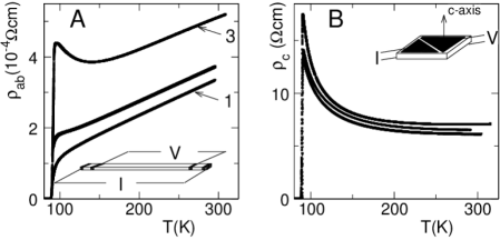
Figure 15: In-plane (A) and out-of-plane (B) resistivity of 3 single crystals of Bi₂Sr₂CaCu₂O₈ zavale showing no signature of phase fluctuations above the resistive transition.

Both in-plane buc ; mac0 ; boz ; lawrie ; gan and out-of-plane alezavnev ; hof2 ; zve resistive transitions of high-quality samples are sharp and remain sharp in the magnetic field providing a reliable determination of the genuine $H_{c2}(T)$. The vortex entropy cap estimated from the Nernst signal is an order of magnitude smaller than the difference between the entropy of the superconducting state and the extrapolated entropy of the normal state obtained from the specific heat. The preformed Cooper-pair model kiv is incompatible with a great number of thermodynamic, magnetic, and kinetic measurements, which show that only holes (density x), doped into a parent insulator are carriers both in the normal and the superconducting states of cuprates. The assumption kiv that the superfluid density is small compared with the normal-state carrier density is also inconsistent with the theorem pop , which proves that the number of supercarriers at $T=0$K should be the same as the number of normal-state carriers in any clean superfluid.

Recently we described the unusual Nernst signal in cuprates in a different manner as the normal state phenomenon alezav . We have also extended this description to cuprates with very low doping level accounting for their Nernst signal, the thermopower and the insulating-like in-plane low temperature resistance alecon as observed xu ; cap ; cap2 .

Thermomagnetic effects appear in conductors subjected to a longitudinal temperature gradient $\nabla_{x}T$ in $x$ direction and a perpendicular magnetic field in $z$ direction. The transverse Nernst-Ettingshausen effect nernst (here the Nernst effect) is the appearance of a transverse electric field $E_{y}$ in the third direction. When bipolarons are formed in the strong-coupling regime, the chemical potential is negative, Eq.(73). It is found in the impurity band just below the mobility edge at $T>T_{c}$. Carriers, localized below the mobility edge contribute to the longitudinal transport together with the itinerant carriers in extended states above the mobility edge. Importantly the contribution of localized carriers of any statistics to the transverse transport is normally small ell since a microscopic Hall voltage will only develop at junctions in the intersections of the percolation paths, and it is expected that these are few for the case of hopping conduction among disorder-localized states mott2 . Even if this contribution is not negligible, it adds to the contribution of itinerant carriers to produce a large Nernst signal, $e_{y}(T,B)\equiv-E_{y}/\nabla_{x}T$, while it reduces the thermopower $S$ and the Hall angle $\Theta$. This unusual ”symmetry breaking” is completely at variance with ordinary metals where the familiar ”Sondheimer” cancelation sond makes $e_{y}$ much smaller than $S\tan\Theta$ because of the electron-hole symmetry near the Fermi level. Such behavior originates in the ”sign” (or ”$p-n$”) anomaly of the Hall conductivity of localized carriers. The sign of their Hall effect is often $opposite$ to that of the thermopower as observed in many amorphous semiconductors ell and described theoretically fri .

The Nernst signal is expressed in terms of the kinetic coefficients $\sigma_{ij}$ and $\alpha_{ij}$ as

$$e_{y}={\frac{{\sigma_{xx}\alpha_{yx}-\sigma_{yx}\alpha_{xx}}}{{\sigma_{xx}^{2}+\sigma_{xy}^{2}}}},$$ (78)

where the current density is given by $j_{i}=\sigma_{ij}E_{j}+\alpha_{ij}\nabla_{j}T$. When the chemical potential $\mu$ is at the mobility edge, localized carriers contribute to the transport, so $\sigma_{ij}$ and $\alpha_{ij}$ in Eq.(77) can be expressed as $\sigma^{ext}_{ij}+\sigma^{l}_{ij}$ and $\alpha^{ext}_{ij}+\alpha^{l}{ij}$, respectively. Since the Hall mobility of carriers localized below $\mu$, $\sigma^{l}_{yx}$, has the sign opposite to that of carries in the extended states above $\mu$, $\sigma^{ext}_{yx}$, the sign of the off-diagonal Peltier conductivity $\alpha^{l}_{yx}$ should be the same as the sign of $\alpha^{ext}_{yx}$. Then neglecting the magneto-orbital effects in the resistivity (since $\Theta\ll 1$ xu ) we obtain

$$S\tan\Theta\equiv{\sigma_{yx}\alpha_{xx}\over{\sigma_{xx}^{2}+\sigma_{xy}^{2}}}\approx\rho(\alpha^{ext}_{xx}-|\alpha^{l}_{xx}|)(\Theta^{ext}-|\Theta^{l}|)$$ (79)

and

$$e_{y}\approx\rho(\alpha^{ext}_{yx}+|\alpha^{l}_{yx}|)-S\tan\Theta,$$ (80)

where $\Theta^{ext}\equiv\sigma^{ext}_{yx}/\sigma_{xx}$, $\Theta^{l}\equiv\sigma^{l}_{yx}/\sigma_{xx}$, and $\rho=1/\sigma_{xx}$ is the resistivity.

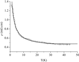
Figure 16: Normal state in-plane resistivity of underdoped La_1.94 Sr_0.06CuO₄ (triangles cap ) as revealed in the field $B=12$ Tesla and compared with the bipolaron theory, Eq.(82) (solid line).

Clearly the model, Eqs.(78,79) can account for a low value of $S\tan\Theta$ compared with a large value of $e_{y}$ in some underdoped cuprates xu ; cap2 due to the sign anomaly. Even in the case when localized bosons contribute little to the conductivity their contribution to the thermopower $S=\rho(\alpha^{ext}_{xx}-|\alpha^{l}_{xx}|))$ could almost cancel the opposite sign contribution of itinerant carriers alezav . Indeed the longitudinal conductivity of itinerant two-dimensional bosons, $\sigma^{ext}\propto\int_{0}dEEdf(E)/dE$ diverges logarithmical when $\mu$ in the Bose-Einstein distribution function $f(E)=[\exp((E-\mu)/T)-1]^{-1}$ goes to zero and the relaxation time $\tau$ is a constant. At the same time $\alpha^{ext}_{xx}\propto\int_{0}dEE(E-\mu)df(E)/dE$ remains finite, and it could have the magnitude comparable with $\alpha^{l}_{xx}$. Statistics of bipolarons gradually changes from Bose to Fermi statistics with lowering energy across the mobility edge because of the Coulomb repulsion of bosons in localized states alegile . Hence one can use the same expansion near the mobility edge as in ordinary amorphous semiconductors to obtain the familiar textbook result $S=S_{0}T$ with a constant $S_{0}$ at low temperatures mott3 . The model becomes particularly simple, if we neglect the localized carrier contribution to $\rho$, $\Theta$ and $\alpha_{xy}$, and take into account that $\alpha^{ext}_{xy}\propto B/\rho^{2}$ and $\Theta^{ext}\propto B/\rho$ in the Boltzmann theory. Then Eqs.(78,79) yield

$$S\tan\Theta\propto T/\rho$$ (81)

and

$$e_{y}(T,B)\propto(1-T/T_{1})/\rho.$$ (82)

According to our earlier suggestion alelog the insulating-like low-temperature dependence of $\rho(T)$ in underdoped cuprates originates from the elastic scattering of nondegenerate itinerant carriers off charged impurities. We assume here that the carrier density is temperature independent at low temperatures in agreement with the temperature-independent Hall effect per . The relaxation time of nondegenerate carriers depends on temperature as $\tau\propto T^{-1/2}$ for scattering off short-range deep potential wells, and as $T^{1/2}$ for very shallow wells alelog . Combining both scattering rates we obtain

$$\rho=\rho_{0}[(T/T_{2})^{1/2}+(T_{2}/T)^{1/2}].$$ (83)

Eq.(82) with $\rho_{0}=0.236$ m$\Omega\cdot$cm and $T_{2}=44.6$K fits extremely well the experimental insulating-like normal state resistivity of underdoped La_1.94 Sr_0.06CuO₄ in the whole low-temperature range from 2K up to 50K, Fig.16, as revealed in the field $B=12$ Tesla cap ; cap2 . Another high quality fit can be obtained combining the Brooks-Herring formula for the 3D scattering off screened charged impurities, as proposed in Ref.kast for almost undoped $LSCO$, or the Coulomb scattering in 2D ($\tau\propto T$) and a temperature independent scattering rate off neutral impurities with the carrier exchange erg similar to the scattering of slow electrons by hydrogen atoms in three dimensions. Hence the scale $T_{2}$, which determines the crossover toward an insulating behavior, depends on the relative strength of two scattering mechanisms. Importantly our expressions (80,81) for $S\tan\Theta$ and $e_{y}$ do not depend on the particular scattering mechanism. Taking into account the excellent fit of Eq.(82) to the experiment, they can be parameterized as

$$S\tan\Theta=e_{0}{(T/T_{2})^{3/2}\over{1+T/T_{2}}},$$ (84)

and

$$e_{y}(T,B)=e_{0}{(T_{1}-T)(T/T_{2})^{1/2}\over{T_{2}+T}},$$ (85)

where $T_{1}$ and $e_{0}$ are temperature independent.

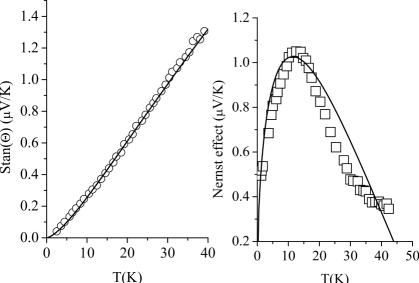
Figure 17: $S\tan\Theta$ (circles cap2 ) and the Nernst effect $e_{y}$ (squares cap ) of underdoped La_1.94 Sr_0.06CuO₄ at $B=12$ Tesla compared with the bipolaron theory, Eqs.(18,19) (solid lines).

In spite of all simplifications, the model describes remarkably well both $S\tan\Theta$ and $e_{y}$ measured in La_1.94 Sr_0.06CuO₄ with a $single$ fitting parameter, $T_{1}=50$K using the experimental $\rho(T)$. The constant $e_{0}=2.95$ $\mu$V/K scales the magnitudes of $S\tan\Theta$ and $e_{y}$. The magnetic field $B=12$ Tesla destroys the superconducting state of the low-doped La_1.94 Sr_0.06CuO₄ down to $2$K, Fig.16, so any residual superconducting order above $2$K is clearly ruled out, while the Nernst signal, Fig.17, is remarkably large. The coexistence of the large Nernst signal and a nonmetallic resistivity is in sharp disagreement with the vortex scenario, but in agreement with our model. Taking into account the field dependence of the conductivity of localized carriers, the phonon-drug effect, and their contribution to the transverse magnetotransport can well describe the magnetic field dependence of the Nernst signal alezav and improve the fit in Fig.17 at the expense of the increasing number of fitting parameters.

IV.3 Normal state diamagnetism

A number of experiments (see, for example, mac ; junM ; hof ; nau ; igu ; ong and references therein), including torque magnetometries, showed enhanced diamagnetism above $T_{c}$, which has been explained as the fluctuation diamagnetism in quasi-2D superconducting cuprates (see, for example Ref. hof ). The data taken at relatively low magnetic fields (typically below 5 Tesla) revealed a crossing point in the magnetization $M(T,B)$ of most anisotropic cuprates (e.g. $Bi-2212$), or in $M(T,B)/B^{1/2}$ of less anisotropic $YBCO$ junM . The dependence of magnetization (or $M/B^{1/2}$) on the magnetic field has been shown to vanish at some characteristic temperature below $T_{c}$. However the data taken in high magnetic fields (up to 30 Tesla) have shown that the crossing point, anticipated for low-dimensional superconductors and associated with superconducting fluctuations, does not explicitly exist in magnetic fields above 5 Tesla nau .

Most surprisingly the torque magnetometery mac ; nau uncovered a diamagnetic signal somewhat above $T_{c}$ which increases in magnitude with applied magnetic field. It has been linked with the Nernst signal and mobile vortexes in the normal state of cuprates ong . However, apart from the inconsistences mentioned above, the vortex scenario of the normal-state diamagnetism is internally inconsistent. Accepting the vortex scenario and fitting the magnetization data in $Bi-2212$ with the conventional logarithmic field dependence ong , one obtains surprisingly high upper critical fields $H_{c2}>120$ Tesla and a very large Ginzburg-Landau parameter, $\kappa=\lambda/\xi>450$ even at temperatures close to $T_{c}$. The in-plane low-temperature magnetic field penetration depth is $\lambda=200$ nm in optimally doped $Bi-2212$ (see, for example tallon ). Hence the zero temperature coherence length $\xi$ turns out to be about the lattice constant, $\xi=0.45$nm, or even smaller. Such a small coherence length rules out the ”preformed Cooper pairs” kiv , since the pairs are virtually not overlapped at any size of the Fermi surface in $Bi-2212$ . Moreover the magnetic field dependence of $M(T,B)$ at and above $T_{c}$ is entirely inconsistent with what one expects from a vortex liquid. While $-M(B)$ decreases logarithmical at temperatures well below $T_{c}$, the experimental curves mac ; nau ; ong clearly show that $-M(B)$ increases with the field at and above $T_{c}$ , just opposite to what one could expect in the vortex liquid. This significant departure from the London liquid behavior clearly indicates that the vortex liquid does not appear above the resistive phase transition mac .

Some time ago we explained the anomalous diamagnetism in cuprates as the Landau normal-state diamagnetism of preformed bosons den . The same model predicted the unusual upper critical field aleH observed in many superconducting cuprates buc ; mac0 ; boz ; lawrie ; gan ; alezavnev ; ZAV (see below). Here we extend the model to high magnetic fields taking into account the magnetic pair-breaking of singlet bipolarons and the anisotropy of the energy spectrum. When the strong magnetic field is applied perpendicular to the copper-oxygen plains the quasi-2D bipolaron energy spectrum is quantized as

$$E_{\alpha}=\omega(n+1/2)+2t_{c}[1-\cos(K_{z}d)],$$ (86)

where $\omega=2eB/m_{b}$, $n=0,1,2,...$, and $t_{c}$, $K_{z}$, $d$ are the hopping integral, the momentum and the lattice period perpendicular to the planes. Quantum numbers $\alpha$ also include the momentum along one of the in-plane directions. Expanding the Bose-Einstein distribution function in powers of $exp[(\mu-E_{\alpha})/T]$ with the negative $\mu$ one can readily obtain (after summation over $n$) the boson density

$$n_{b}={eB\over{\pi d}}\sum_{k=1}^{\infty}I_{0}(2t_{c}k/T){\exp[(\tilde{\mu}-2t_{c})k/T]\over{1-\exp(-\omega k/T)}},$$ (87)

and the magnetization

$$M(T,B) = -n_{b}\mu_{b}+{eT\over{\pi d}}\sum_{k=1}^{\infty}I_{0}(2t_{c}k/T){\exp[(\tilde{\mu}-2t_{c})k/T]\over{1-\exp(-\omega k/T)}}$$ (88)

$$\times \left({1\over{k}}-{\omega\exp(-\omega k/T)\over{T[1-\exp(-\omega k/T)]}}\right),$$ (89)

where $\mu_{b}=e/m_{b}$, $\tilde{\mu}=\mu-\omega/2$ and $I_{0}(x)$ is the modified Bessel function. At low temperatures $T\rightarrow 0$ Schafroth’s result sha is recovered, $M(0,B)=-n_{b}\mu_{b}$. The magnetization of charged bosons is field-independent at low temperatures. At high temperatures, $T\gg T_{c}$ the chemical potential has a large magnitude , so we can keep only terms with $k=1$ in Eqs.(86,87) to obtain

$$M(T,B)=-n_{b}\mu_{b}+{Tn_{b}\over{B}}\left(1-{\omega\exp(-\omega/T)\over{T[1-\exp(-\omega/T)]}}\right).$$ (90)

The experimental conditions are such that $T\gg\omega$ when $T$ is of the order of $T_{c}$ or higher, so that

$$M(T,B)=-n_{b}\mu_{b}{\omega\over{6T}},$$ (91)

which is the Landau orbital diamagnetism of nondegenerate carriers. The bipolaron in-plane mass in cuprates is about $m_{b}\approx 10m_{e}$ alebook1 . Using this mass yields $M(0,B)\approx 2000$ A/m with the bipolaron density $n_{b}=10^{21}$ cm^-3. Then the magnitude and the field/temperature dependence of $M(T,B)$ near and above $T_{c}$ are about the same as experimentally observed in Refs nau ; ong .

The pseudogap temperature $T^{*}$ depends on the magnetic field predominantly because of the magnetic-field splitting of the single-polaron band in Fig.12. As a result the bipolaron density depends on the field (as well as on temperature) near $T_{c}$ as

$$n_{b}(T,B)=n_{b}(T_{c},0)\left[1+(T_{c}-T)/\tilde{T}_{0}-(B/B_{0})^{\beta}\right],$$ (92)

where $\tilde{T}_{0}$ and $B_{0}$ are constants depending on $T^{*}$, $\beta=2$ if the polaron spectrum is spin-degenerate, and $\beta=1$ if the spin degeneracy is removed by the crystal field already in the absence of the external field.

Theoretical temperature and field dependencies of $M(T,B)$, Eq.(87) agree qualitatively with the experimental curves in $Bi-2212$ nau ; ong , if the depletion of the bipolaron density, Eq.(90) is taken into account. The depletion of $n_{b}$ accounts for the absence of the crossing point in $M(T,B)$ at high magnetic fields. Nevertheless a quantitative fit to experimental $M(T,B)$ curves using $\tilde{T}_{0}$ and $B_{0}$ as the fitting parameters is premature. The experimental diamagnetic magnetization has been extracted from the total magnetization assuming that the normal state paramagnetic contribution remains temperature-independent at all temperatures nau ; ong . This assumption is inconsistent with a great number of NMR and the Knight shift measurements, and even with the preformed Cooper-pair model itself. The Pauli spin-susceptibility has been found temperature-dependent in these experiments revealing normal-state pseudogaps, contrary to the assumption. Hence the experimental diamagnetic $M(T,B)$ nau ; ong has to be corrected by taking into account the temperature dependence of the spin paramagnetism at relatively low temperatures.

IV.4 Spin pseudogap, $c$-axis transport and charge pseudogap

The pairing of holes into singlets well above $T_{c}$ should be seen as a drop of the nuclear magnetic relaxation rate $1/T_{1}$ with temperature lowering. Indeed it is a common feature of the normal state of many cuprates. The bipolaron model has described the temperature dependence of $1/T_{1}$ alegap . The conventional contact hyperfine coupling of nuclear spin on a site $i$ with electron spins is given in the site representation by

$$H_{i}=\hat{A}_{i}\sum_{j}c_{j\uparrow}^{\dagger}c_{j\downarrow}+H.c.,$$ (93)

where $\hat{A}_{i}$ is an operator acting on the nuclear spin, and $j$ is its nearest neighbor sites. Performing projecting transformations to bipolarons as above we obtain the effective spin-flip interaction of triplet bipolarons with the nuclear spin as

$$H_{i}\sim\sum_{j,l\neq l^{\prime}}b_{j,l}^{\dagger}b_{j,l^{\prime}}+H.c.$$ (94)

Here $l,l^{\prime}=0,\pm 1$ are z-components of spin $S=1$. The NMR width due to the spin-flip scattering of triplet bipolarons on nuclei is obtained using the Fermi-Dirac golden rule,

$${\frac{1}{{T_{1}}}}=-\frac{B}{t^{2}}\int_{0}^{2t}dE\frac{\partial f(E)}{\partial E}$$ (95)

where $f(E)=[\exp((E+J-\mu)/T)-]^{-1}$ is the triplet distribution function, and $2t$ is their bandwidth. For simplicity the triplet DOS is taken as a constant ($=1/(2t)$). As a result, we obtain

$${\frac{1}{{T_{1}}}}={\frac{BT\sinh(t/T)}{{t^{2}[\cosh[(t+J)/T-\ln y]-\cosh(t/T)]}},}$$ (96)

where $B$ is a temperature independent hyperfine coupling constant.

Eq.(94) describes all essential features of the nuclear spin relaxation rate in copper-based oxides: the absence of the Hebel-Slichter coherent peak below $T_{c}$, the temperature-dependent Korringa ratio ($1/TT_{1}$) above $T_{c}$, and a large value of $1/T_{1}$ due to the small bandwidth 2$t$. It nicely fits the experimental data in $YBa_{2}Cu_{4}O_{8}$ tan with reasonable values of the parameters, $t=250$K and $J=150$K alegap . A similar unusual behavior of NMR was found in underdoped $YBa_{2}Cu_{3}O_{6+x}$, and in many other cuprates. The Knight shift, which measures the spin susceptibility of carriers, also drops well above $T_{c}$ in many copper oxides, in agreement with the bipolaron model. The ‘spin’ gap has been observed above and below $T_{c}$ in $YBa_{2}Cu_{3}O_{6+x}$ with unpolarized ros , and polarized moo neutron scattering.

The bipolaron model has also quantitatively explained $c$-axis transport and the anisotropy of cuprates alekabmot ; in ; hof2 ; zve . The crucial point is that single polarons dominate in $c$-axis transport at finite temperatures because they are much lighter than bipolarons in $c$-direction. Bipolarons can propagate across the planes due to a simultaneous two-particle tunnelling alone, which is much less probable than a single polaron tunnelling. Along the planes polarons and inter-site bipolarons propagate with comparable effective masses, as shown above. Hence in the mixture of nondegenerate quasi-two-dimensional bosons and thermally excited fermions, only fermions contribute to $c$ -axis transport, if the temperature is not very low, which leads to thermally activated $c$ -axis transport and to a fundamental relation between the anisotropy and the uniform magnetic susceptibility of cuprates alekabmot .

The exponential temperature dependence of c-axis resistivity and $"c"$ versus $"ab"$ anisotropy was interpreted within the framework of the bipolaron model in many cuprates, in particular in $La_{2-x}Sr_{x}CuO_{4}$ alekabmot ; zhaomul , $Bi_{2}Sr_{2}CaCu_{2}O_{8+\delta}$ in , $YBa_{2}Cu_{3}O_{6+x}$ zve , and $HgBa_{2}CuO_{4+\delta}$ hof2 . Importantly, the uniform magnetic susceptibility above $T_{c}$ increases with doping. It proves once more that cuprates are doped insulators, where low energy charge and spin degrees of freedom are due to holes doped into a parent insulating matrix with no free carriers and no free spins. A rather low magnetic susceptibility of parent insulators in their paramagnetic phase is presumably due to a singlet pairing of copper spins.

V Superconducting state of cuprates

V.1 Parameter-free evaluation of $T_{c}$: Bose-Einstein condensation versus the Kosterlitz-Thouless transition

An ultimate goal of the theory of superconductivity is to provide an expression for $T_{c}$ as a function of some well-defined parameters characterizing the material. In the framework of the BCS theory $T_{c}$ is fairly approximated by the familiar McMillan’s formula, which works well for simple metals and their alloys. But applying a theory of this kind to high-T_c cuprates is problematic. Since bare electron bands are narrow, strong correlations result in the Mott insulating state of undoped parent compounds. As a result, $\mu^{\ast}$ is ill-defined in doped cuprates, and polaronic effects are important as in many doped semiconductors. Hence, an estimate of $T_{c}$ in cuprates within the BCS theory appears to be an exercise in calculating the Coulomb pseudopotential $\mu^{\ast}$ rather than $T_{c}$ itself. One cannot increase $\lambda$ either without accounting for a polaron collapse of the band as discussed above. This appears at $\lambda\approx 1$.

On the other hand, the bipolaron theory provides a parameter-free expression for $T_{c}$ alekabTc , which fits the experimentally measured $T_{c}$ in many cuprates for any level of doping. $T_{c}$ is calculated using the density sum rule as the Bose-Einstein condensation (BEC) temperature of $2e$ charged bosons on a lattice. Just before the discovery mul we predicted $T_{c}$ as high as $\approx 100K$ using an estimate of the bipolaron effective mass alekab0 . Uemura uem established a correlation of $T_{c}$ with the in-plane magnetic field penetration depth measured by $\mu sR$ technique in many cuprates as $T_{c}\sim 1/\lambda_{ab}^{2}$. The technique is based on the implantation of spin polarized muons. It monitors the time evolution of the muon spin polarization. He concluded that cuprates are neither BCS nor BEC superfluids but they are in a crossover region from one to the other, because the experimental $T_{c}$ was found about $3$ or more times below the BEC temperature.

Here we calculate $T_{c}$ of a bipolaronic superconductor taking properly into account the microscopic band structure of bipolarons in layered cuprates as derived in section 3. We arrive at a parameter-free expression for $T_{c},$ which in contrast to Ref. uem involves not only the in-plane, $\lambda_{ab}$ but also the out-of-plane, $\lambda_{c}$, magnetic field penetration depth, and a normal state Hall ratio $R_{H}$ just above the transition. It describes the experimental data for a few dozen different samples, Fig.18, clearly indicating that many cuprates are in the BEC rather than in the crossover regime.

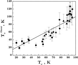
Figure 18: Theoretical critical temperature compared with the experiment (the theory is exact for samples on the straight line) for $LaSrCuO$ compounds (squares), for $Zn$ substituted $YBa_{2}Cu_{1-x}Zn_{x}O_{7}$ (circles), for $YBa_{2}Cu_{3}O_{7-\delta}$ (triangles), and for $HgBa_{2}CuO_{4+\delta}$ (diamonds). Experimental data for the London penetration depth are taken from T. Xiang $et$ $al$, Int. J. Mod. Phys. B12, 1007 (1998) and B. Janossy $et$ $al$, Physica C181, 51 (1991) in $YBa_{2}Cu_{3}O_{7-\delta}$ and $YBa_{2}Cu_{1-x}Zn_{x}O_{7}$; from V.G. Grebennik $et$ $al$, Hyperfine Interactions 61, 1093 (1990) and C. Panagopoulos (private communication) in underdoped and overdoped $La_{2-x}Sr_{x}CuO_{4}$, respectively, and from J. Hofer $et$ $al$, Physica C, 297, 103 (1998) in $HgBa_{2}CuO_{4+\delta}$. The Hall coefficient above $T_{c}$ is taken from A. Carrington $et$ $al$, Phys. Rev. B48, 13051 (1993) and J. R. Cooper (private communication) ($YBa_{2}Cu_{3}O_{7-\delta}$ and $YBa_{2}Cu_{1-x}Zn_{x}O_{7}$) and from H.Y. Hwang $et$ $al$, Phys. Rev. Lett. 72, 2636 (1994) ($La_{2-x}Sr_{x}CuO_{4}$).

The energy spectrum of bipolarons is at least two-fold degenerate in cuprates (section 3). One can apply the effective mass approximation at $T\simeq T_{c}$, Eq.(52), because $T_{c}$ should be less than the bipolaron bandwidth. Also three-dimensional corrections to the spectrum are important for the Bose-Einstein condensation. They are well described by the tight-binding approximation as

$$E_{{\bf K}}^{x,y}={\frac{\hbar^{2}K_{x,y}^{2}}{{2m_{x}^{\ast\ast}}}}+{\frac{\hbar^{2}K_{y,x}^{2}}{{2m_{y}^{\ast\ast}}}}+2t_{c}[1-\cos(K_{z}d)].$$ (97)

Substituting the spectrum, Eq.(95) into the density sum rule,

$$\sum_{{\bf K},i=(x,y)}\left[\exp(E_{{\bf K}}^{i}/T_{c})-1\right]^{-1}=n_{b}$$ (98)

one readily obtains $T_{c}$ as (in ordinary units)

$$k_{B}T_{c}=f\left(\frac{t_{c}}{{k_{B}T_{c}}}\right)\times{\frac{3.31\hbar^{2}(n_{b}/2)^{2/3}}{{(m_{x}^{\ast\ast}m_{y}^{\ast\ast}m_{c}^{\ast\ast})^{1/3}}}},$$ (99)

where the coefficient $f(x)\approx 1$ is shown in Fig.19 as a function of the anisotropy, $t_{c}/(k_{B}T_{c})$, and $m_{c}^{\ast\ast}=\hbar^{2}/(2|t_{c}|d^{2})$.

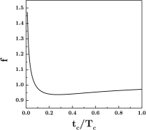
Figure 19: Correction coefficient to the 3D Bose-Einstein condensation temperature as a function of anisotropy.

This expression is rather ambiguous because the effective mass tensor as well as the bipolaron density $n_{b}$ are not well known. Fortunately, we can express the band-structure parameters via in-plane,

$$\lambda_{ab}=\left[\frac{{m_{x}^{\ast\ast}m_{y}^{\ast\ast}}}{8\pi n_{b}e^{2}({m_{x}^{\ast\ast}+m_{y}^{\ast\ast}})}\right]^{1/2}$$

and out-of-plane penetration depths,

$$\lambda_{c}=\left[\frac{{m_{c}^{\ast\ast}}}{16\pi n_{b}e^{2}}\right]^{1/2}$$

(we use $c=1$). The bipolaron density is expressed through the in-plane Hall ratio (above the transition) as

$$R_{H}={\frac{1}{{2en_{b}}}}\times{\frac{4{m_{x}^{\ast\ast}m_{y}^{\ast\ast}}}{{(m_{x}^{\ast\ast}+m_{y}^{\ast\ast})^{2}}}},$$ (100)

which leads to

$$T_{c}=1.64f\left(\frac{{t_{c}}}{{k_{B}T_{c}}}\right)\left({\frac{eR_{H}}{{\lambda_{ab}^{4}\lambda_{c}^{2}}}}\right)^{1/3}.$$ (101)

Here $T_{c}$ is measured in Kelvin, $eR_{H}$ in cm³ and $\lambda$ in cm. The coefficient $f$ is about unity in a very wide range of $t_{c}/(k_{B}T_{c})\geq 0.01$, Fig.19. Hence, the bipolaron theory yields a parameter-free expression, which unambiguously tells us how near cuprates are to the BEC regime,

$$T_{c}\approx T_{c}(3D)=1.64\left({\frac{eR_{H}}{{\lambda_{ab}^{4}\lambda_{c}^{2}}}}\right)^{{1/3}}.$$ (102)

Table 2: Experimental data on $T_{c}$(K), $ab$ and $c$ penetration depth($nm$), Hall coefficient ($10^{-3}(cm^{3}/C)$), and calculated values of $T_{c}$ respectively for $La_{2-x}Sr_{x}CuO_{4}$ ($La$), $YBaCuO(x\%Zn)$ ($Zn$), $YBa_{2}Cu_{3}O_{7-x}$ ($Y$) and $HgBa_{2}CuO_{4+x}$ ($Hg$) compounds

Compound	$T^{exp}_{c}$	$\lambda_{ab}$	$\lambda_{c}$	$R_{H}$,	$T_{c}(3D)$	$T_{c}$	$T_{KT}$
$La$(0.2)	36.2	200	2540	0.8	38	41	93
$La$(0.22)	27.5	198	2620	0.62	35	36	95
$La$(0.24)	20.0	205	2590	0.55	32	32	88
$La$(0.15)	37.0	240	3220	1.7	33	39	65
$La$(0.1)	30.0	320	4160	4.0	25	31	36
$La$(0.25)	24.0	280	3640	0.52	17	19	47
$Zn$(0)	92.5	140	1260	1.2	111	114	172
$Zn$(2)	68.2	260	1420	1.2	45	46	50
$Zn$(3)	55.0	300	1550	1.2	35	36	38
$Zn$(5)	46.4	370	1640	1.2	26	26	30
$Y$(0.3)	66.0	210	4530	1.75	31	51	77
$Y$(0.43)	56.0	290	7170	1.45	14	28	40
$Y$(0.08)	91.5	186	1240	1.7	87	88	98
$Y$(0.12)	87.9	186	1565	1.8	75	82	97
$Y$(0.16)	83.7	177	1557	1.9	83	89	108
$Y$(0.21)	73.4	216	2559	2.1	47	59	73
$Y$(0.23)	67.9	215	2630	2.3	46	58	73
$Y$(0.26)	63.8	202	2740	2.0	48	60	83
$Y$(0.3)	60.0	210	2880	1.75	43	54	77
$Y$(0.35)	58.0	204	3890	1.6	35	50	82
$Y$(0.4)	56.0	229	4320	1.5	28	42	65
$Hg$(0.049)	70.0	216	16200	9.2	23	60	115
$Hg$(0.055)	78.2	161	10300	8.2	43	92	206
$Hg$(0.055)	78.5	200	12600	8.2	28	69	134
$Hg$(0.066)	88.5	153	7040	6.85	56	105	229

Table 3: Mass enhancement in cuprates

Compound	$m_{ab}$	$m_{c}$
$La$(0.2)	22.1	3558
$La$(0.15)	15.0	2698
$La$(0.1)	11.3	1909
$Y$(0.0)	7.2	584
$Y$(0.12)	8.3	600
$Y$(0.3)	10.6	1994

We compare two last expressions with the experimental $T_{c}$ of more than $30$ different cuprates, for which both $\lambda_{ab}$ and $\lambda_{c}$ are measured along with $R_{H}(T_{c}+0)$ in Table 2 and Fig.18. The Hall ratio has a strong temperature dependence above $T_{c}$. Therefore, we use the experimental Hall ratio just above the transition. In a few cases (mercury compounds), where $R_{H}(T_{c}+0)$ is unknown, we take the inverse chemical density of carriers (divided by $e$) as $R_{H}$. For almost all samples the theoretical $T_{c}$ fits experimental values within an experimental error bar for the penetration depth (about $\pm 10\%$). There are a few ${Zn}$ doped YBCO samples, Fig.18, whose critical temperature is higher than the theoretical estimate. If we assume that the degeneracy of the bipolaron spectrum is removed by the random potential of $Zn$, then the theoretical $T_{c}$ would be almost the same as the experimental values for these samples as well.

One can argue that due to a large anisotropy cuprates may belong to a 2D ‘$XY$’ universality class with the Kosterlitz-Thouless  (KT) critical temperature $T_{KT}$ of preformed bosons ald ; poc or the Cooper pairs kiv . Should it be the case, one would hardly discriminate the Cooper pairs with respect to bipolarons. KT critical temperature is expressed through the in-plane penetration depth alone as kiv

$$k_{B}T_{KT}\approx{\frac{0.9d\hbar^{2}}{{16\pi e^{2}\lambda_{ab}^{2}}}}.$$ (103)

It appears significantly higher than the experimental values in many cases (see Table 2). There are also quite a few samples with about the same ${\lambda_{ab}}$ and the same $d$, but with very different values of $T_{c},$ which proves that the phase transition is not the KT transition. On the contrary, our parameter-free fit of the experimental critical temperature and the critical behavior (see below) favor $3D$ Bose-Einstein condensation of charged bosons as the mechanism of high T_c rather than any low-dimensional phase-fluctuation scenario. The fluctuation theory schn further confirms the three-dimensional character of the phase transition in cuprates. However, it does not mean that all high-temperature superconductors are in the BEC regime with charged bosons as supercarriers. Some of them, in particular, electron-doped cuprates, $MgB_{2}$ and doped fullerenes might be in the BCS or intermediate regime, which makes the BCS-BEC crossover problem to be relevant. Starting from the pioneering works by Eagles eag2 and Legget leg this problem received particular attention in the framework of a negative Hubbard $U$ model noz ; micr . Both analytical (diagrammatic dia , path integral alerub ) and numerical rand studies have addressed the intermediate coupling regime beyond a variational approximation noz , including 2D systems var2 ; rand ; tra . However, in using the negative Hubbard $U$ model, we have to realize that this model, which predicts a smooth BCS-BEC crossover, cannot be applied to the BCS-bipolaron crossover. The essential effect of the polaron band-narrowing (section 2) is missing in the negative (and positive) Hubbard $U$ model. The polaron collapse of the bandwidth is mainly responsible for high $T_{c}$. It strongly affects the BCS-BEC crossover significantly reducing the crossover region.

It is interesting to estimate the effective mass tensor using the penetration depth and the Hall ratio. These estimates for in-plane and out-of-plane boson masses are presented in Table 3. They agree with the inter-site bipolaron mass (section 3). We notice, however, that the absolute value of the effective mass in terms of the free electron mass does not describe the actual band mass renormalization if the bare (band) mass is unknown. Nevertheless an assumption kiv that the number of carriers is determined by the Luttinger theorem (i.e. $n\approx 1$) would lead to much heavier carriers with $m^{\ast}$ about $100m_{e}.$

V.2 Isotope effect on $T_{c}$ and on supercarrier mass

The advances in the fabrication of the isotope substituted samples made it possible to measure a sizable isotope effect , $\alpha=-d\ln T_{c}/d\ln M$ in many high-$T_{c}$ oxides. This led to a general conclusion that phonons are relevant for high $T_{c}$. Moreover the isotope effect in cuprates was found to be quite different from the BCS prediction, $\alpha=0.5$ (or less). Several compounds showed $\alpha>0.5$ cra , and a small negative value of $\alpha$ was found in $Bi-2223$ bor .

Essential features of the isotope effect, in particular large values in low $T_{c}$ cuprates, an overall trend to lower value as $T_{c}$ increases fra , and a small or even negative $\alpha$ in some high $T_{c}$ cuprates were understood in the framework of the bipolaron theory aleiso . With increasing ion mass the bipolaron mass increases and the Bose-Einstein condensation temperature $T_{c}$ decreases in the bipolaronic superconductor. On the contrary in polaronic superconductors an increase of the ion mass leads to a band narrowing and to an enhancement of the polaron density of states, and to an increase of $T_{c}$. Hence the isotope exponent in $T_{c}$ can distinguish the BCS like polaronic superconductivity with $\alpha<0$ , and the Bose-Einstein condensation of small bipolarons with $\alpha>0$. Moreover, underdoped cuprates, which are definitely in the BEC regime, could have $\alpha>0.5,$ as observed.

The isotope effect on $T_{c}$ is linked with the isotope effect on the carrier mass, $\alpha_{m^{*}}$, as aleiso

$$\alpha=-d\ln T_{c}/d\ln M=\alpha_{m^{*}}[1-Z/(\lambda-\mu_{c})],$$ (104)

where $\alpha_{m^{*}}=d\ln m^{*}/d\ln M$ and $Z=m/m^{*}\ll 1$. In ordinary metals, where the Migdal approximation is believed to be valid, the renormalized effective mass of electrons is independent of the ion mass $M$ because the electron-phonon interaction constant $\lambda$ does not depend on $M$. However, when the e-ph interaction is sufficiently strong, the electrons form polarons dressed by lattice distortions, with an effective mass $m^{\ast}=m\exp(\gamma E_{p}/\hbar\omega)$. While $E_{p}$ in the above expression does not depend on the ion mass, the phonon frequency does. As a result, there is a large isotope effect on the carrier mass in polaronic conductors, $\alpha_{m^{*}}=(1/2)\ln(m^{*}/m)$ aleiso , in contrast to the zero isotope effect in ordinary metals.

Such an effect was observed in cuprates in the London penetration depth of isotope-substituted samples zhao . The carrier density is unchanged with the isotope substitution of $O^{16}$ by $O^{18}$, so that the isotope effect on $\lambda_{ab}$ measures directly the isotope effect on the carrier mass. In particular, the carrier mass isotope exponent $\alpha_{m^{*}}$ was found as large as $\alpha_{m^{*}}=0.8$ in $La_{1.895}Sr_{0.105}CuO_{4}$. Then the polaron mass enhancement should be $m^{\ast\ast}/m\approx 5$ in this material. Using Eq.(57) we obtain the in-plane bipolaron mass as large as $m^{\ast\ast}\approx 10m_{e}$ with the bare hopping integral $T(NNN)=0.2$ eV. The in-plane magnetic field penetration depth, calculated with this mass is    $\lambda_{ab}=[m^{\ast\ast}/8\pi ne^{2}]^{1/2}\approx 316$nm, where $n$ is the hole density. It agrees well with the experimental one, $\lambda_{ab}\simeq 320$nm. Using the measured values of $\ \lambda_{ab}=320$ nm, $\lambda_{c}=4160$ nm, and of $R_{H}=4\times 10^{-3}$ $cm^{3}/C$ (just above $T_{c}$) we obtain $T_{c}=31K$ from Eq.(100) in astonishing agreement with the experimental value $T_{c}=30$ $K$ in this compound. More recent high resolution angle resolved photoemission spectroscopy studies LAN provided further compelling evidence for strong e-ph interaction in the cuprates. They revealed a fine phonon structure in the electron self-energy of underdoped La_2-xSr_xCuO₄ samples and a complicated isotope effect in the electron spectral function of Bi2212 that depended on the electron energy and momentum.

V.3 Specific heat anomaly

Bose liquids (or more precisely $He^{4}$) show the characteristic $\lambda$ -point singularity of their specific heat, but superfluid Fermi liquids like BCS superconductors exhibit a sharp second order phase transition accompanied by a finite jump in the specific heat. It was established beyond doubt fish ; lor ; ind ; jun ; schM that the anomaly in high $T_{c}$ cuprates differs qualitatively from the BSC prediction. As was stressed by Salamon et al.sal the heat capacity is logarithmic near the transition, and consequently, cannot be adequately treated by the mean-field BCS theory even including the gaussian fluctuations. In particular, estimates using the gaussian fluctuations yield an unusually small coherence volume, Table 4, comparable with the unit cell volume lor .

Table 4: Coherence volume $\Omega$ in $\AA^{3}$, the in-plane $\xi_{ab}$ and out- of- plane $\xi_{c}$ coherence lengths derived from a Ginzburg-Landau analysis of the specific heat lor

$Compound$	$\Omega$	$\xi^{2}_{ab}$,$(\AA^{2})$	$\xi_{c}$, ($\AA$)
$YBa_{2}Cu_{3}O_{7}$	400	125	3.2
$YBa_{2}Cu_{3}O_{7-0.025}$	309	119	2.6
$YBa_{2}Cu_{3}O_{7-0.05}$	250	119	2.1
$YBa_{2}Cu_{3}O_{7-0.1}$	143	119	1.2
$Ca_{0.8}Y_{0.2}Sr_{2}Tl_{0.5}Pb_{0.5}Cu_{2}O_{7}$	84	70	1.2
$Tl_{1.8}Ba_{2}Ca_{2.2}Cu_{3}O_{10}$		40	$<0.9$

The magnetic field dependence of the anomaly jun0 is also unusual, but it can be described by the bipolaron model alekablia ; ZAV . Calculations of the specific heat of charged bosons in a magnetic field require an analytical DOS, $N(\epsilon,B)$ of a particle, scattered by other particles and/or by a random potential of impurities. One can use DOS in the magnetic field with an impurity scattering calculated in the non-crossing approximation aleH . The specific heat coefficient

$$\frac{C(T,B)}{T}=\frac{d}{TdT}\int d\epsilon\frac{N(\epsilon,B)\epsilon}{\exp[(\epsilon-\mu)/T]-1},$$ (105)

calculated with this DOS and with $\mu$ determined from $n_{b}=\int d\epsilon N(\epsilon,B)f(\epsilon)$, is shown in Fig.20. The broad maximum at $T\approx T_{c}$ is practically the same as in the ideal Bose gas without scattering. It barely shifts in the magnetic field. However, there is the second anomaly at lower temperatures, which is absent in the ideal gas. It shifts with the magnetic field, tracing precisely the resistive transition, as clearly seen from the difference between the specific heat in the field and zero-field curve, Fig.20b.

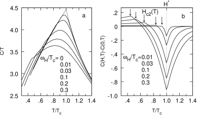
Figure 20: Temperature dependence of the specific heat divided by temperature (arb. units) of the charged Bose-gas scattered by impurities for several fields ($\omega_{H}=2eB/m^{\ast\ast})$. (b) shows two anomalies, the lowest one traces resistive transition, while the highest anomaly is the normal state feature.

The specific heat, Fig. 20, is in striking resemblance with the Geneva group’s experiments on $DyBa_{2}Cu_{3}0_{7}$ and on $YBa_{2}Cu_{3}O_{7}$ jun0 , where both anomalies were observed. Within the bipolaron model, when the magnetic field is applied, it hardly changes the temperature dependence of the chemical potential near the zero field $T_{c}$ because the energy spectrum of thermally excited bosons is practically unchanged. This is because their characteristic energy (of the order of $T_{c}$) remains huge compared with the magnetic energy of the order of $2eB/m^{\ast\ast}$. In contrast, the energy spectrum of low energy bosons is strongly perturbed even by a weak magnetic field. As a result the chemical potential ‘touches’ the band edge at lower temperatures, while having almost the same ‘kink’-like temperature dependence around $T_{c}$ as in zero field. While the lower anomaly corresponds to the true long-range order due to the Bose-Einstein condensation, the higher one is just a ‘memory’ about the zero-field transition. This microscopic consideration shows that a genuine phase transition into a superconducting state is related to a resistive transition, and to the lower specific heat anomaly, while the broad higher anomaly is a normal state feature of the bosonic system in the external magnetic field. Different from the BCS superconductor these two anomalies are well separated in the bosonic superconductor at any field but zero.

V.4 Universal upper critical field

The upper critical field, $H_{c2}(T)=\Phi_{0}/2\pi\xi(T)^{2}$, is very different in the BCS superconductor and in the charged Bose-gas (CBG). While $H_{c2}(T)$ is linear in temperature near $T_{c}$ in the Landau theory of second-order phase transitions, it has a positive curvature $H_{c2}(T)\sim(T_{c}-T)^{3/2}$ in CBG aleH . Also at zero temperature $H_{c2}(0)$ is normally below the Pauli pair-breaking limit given by $H_{p}\simeq 1.84T_{c}$ (in Tesla) in the BCS theory, but the limit can be exceeded by many times in CBG.

In cuprates buc ; mac0 ; boz ; lawrie ; gan ; alezav ; ZAV , spin-ladders spin and organic superconductors org high magnetic field studies revealed a non-BCS upward curvature of resistive $H_{c2}(T)$. When measurements were performed on low-T_c unconventional superconductors mac0 ; boz ; lawrie ; spin ; org , the Pauli limit was exceeded by several times. A non-linear temperature dependence in the vicinity of $\ T_{c}$ was unambiguously observed in a few samples alezav ; lawrie ; gan ; ZAV . Importantly, a thermodynamically determined $H_{c2}$ turned out much higher than the resistive $H_{c2}$ wen due to contrasting magnetic field dependencies of the specific heat anomaly and of resistive transition.

I believe that many unconventional superconductors are in the ‘bosonic’ limit of preformed real-space bipolarons, so their resistive $H_{c2}$ is actually a critical field of the Bose-Einstein condensation of charged bosons aleH . Calculations above carried out for the heat capacity of CBG lead to the conclusion that the resistive $H_{c2}$ and the thermodynamically determined $H_{c2}$ are very different in bosonic superconductors. While the magnetic field destroys the condensate of ideal bosons, it hardly shifts the specific heat anomaly as observed.

A comprehensive scaling of resistive $H_{c2}$ measurements in unconventional superconductors is shown in Fig.21 ZAV in the framework of the microscopic model of charged bosons scattered by impurities. An expression for $H_{c2}(T)$ accounting for a temperature dependence of the number of delocalized bosons, $n_{b}(T),$ can be written as ZAV

$$H_{c2}(T)=H_{0}\left[\frac{n_{b}(T)}{tn_{b}(T_{c})}-t^{1/2}\right]^{3/2},$$ (106)

where $T_{c}$ is the zero-field critical temperature, and $t=T/T_{c}$. Here the scaling constant $H_{0}$ depends on the mean-free path $l$ , $H_{0}=\Phi_{0}/2\pi\xi_{0}^{2}$, with the characteristic (coherence) length $\xi_{0}\simeq(l/n_{b}(T_{c}))^{1/4}$. In the vicinity of $T_{c}$ one obtains the parameter-free $H_{c2}(T)\propto(1-t)^{3/2}$ using this equation, but the low-temperature behavior depends on a particular scattering mechanism, and a detailed structure of the density of localized states. As suggested by the normal state Hall measurements in cuprates $n_{b}(T)$ can be parameterized as $n_{b}(T)=n_{b}(0)+constant\times T$ (see also Eq.(62)), so that $H_{c2}(T)$ is described by a single-parameter expression as

$$H_{c2}(T)=H_{0}\left[\frac{b(1-t)}{t}+1-t^{1/2}\right]^{3/2}.$$ (107)

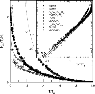
Figure 21: Resistive upper critical field (determined at 50% of the transition) of cuprates, spin-ladders and organic superconductors scaled according to Eq.(105) ZAV . The parameter b is 1 (solid line), 0.02 (dashed-dotted line), 0.0012 (dotted line), and 0 (dashed line). The inset shows a universal scaling of the same data near $T_{c}$ on the logarithmic scale.

The parameter $b$ is proportional to the number of delocalized bosons at zero temperature. We expect that this expression is applied in the whole temperature region except ultra-low temperatures, where the non-crossing approximation fails alebeerkab2 . Exceeding the Pauli pair-breaking limit readily follows from the fact, that the singlet-pair binding energy is related to the normal-state pseudogap temperature $T^{\ast}$, rather than to $T_{c}$. $T^{\ast}$ is higher than $T_{c}$ in bosonic superconductors and in cuprates. The universal scaling of $H_{c2}$ near $T_{c}$ is confirmed by resistive measurements of the upper critical field of many cuprates, spin-ladders, and organic superconductors, as shown in Fig.21. All measurements reveal a universal $(1-t)^{3/2}$ behavior in a wide temperature region (inset) near $T_{c}$. The low-temperature behavior of $H_{c2}(T)/H_{0}$ is not universal, but well described using Eq.(105) with the single fitting parameter, $b$. The parameter is close to $1$ in high quality cuprates with a very narrow resistive transition. It naturally becomes rather small in overdoped cuprates where randomness is more essential.

V.5 Symmetry and space modulations of the order parameter

Independent observations of normal state pseudogaps in a number of magnetic and kinetic measurements, and the unusual critical behavior, discussed above, tell us that many cuprates may not be $BCS$ superconductors. Indeed their superconducting state is as anomalous as the normal one. In particular, there is strong evidence for a $d$-like order parameter (changing sign when the $CuO_{2}$ plane is rotated by $\pi/2$) in cuprates ann . A number of phase-sensitive experiments pha provide unambiguous evidence in this direction; furthermore, the low temperature magnetic penetration depth bonn ; xia was found to be linear in a few cuprates as expected for a d-wave BCS superconductor. However, $SIN$ and $SIS$ tunnelling studies, the $c$-axis Josephson tunnelling klem and some high-precision magnetic measurements mulsym show a more usual $s$-like symmetry or even reveal an upturn in the temperature dependence of the penetration depth below some characteristic temperature wal . Also both angle-resolved photoemission (ARPES) shen and scanning tunnelling microscopy (STM) ren have shown that the maximum energy gap and $2\Delta/T_{c}$ ratio is several times larger than expected in the weak-coupling BCS theory, or in its intermediate-coupling Eliashberg generalization. Strong deviations from the Fermi/BCS-liquid behavior are suggestive of a new electronic state in cuprates, which is a charged Bose liquid of bipolarons aleedw .

Actually there are more complicated deviations from the conventional Fermi/BCS-liquid behavior than the normal state pseudogaps. Recent studies of the gap function revealed two distinctly different gaps with different magnetic field and temperature dependence deu ; kras , and the checkerboard spatial modulations of the tunnelling DOS, with hoff and without hoff2 ; kapit applied magnetic fields. We have proposed a simple phenomenological model aleand explaining two different gaps in cuprates. The main assumption, supported by a parameter-free estimate of the Fermi energy (section 3.5), is that the attractive potential is large compared with the renormalized Fermi energy, so that the ground state is the Bose-Einstein condensate of tightly bound real-space pairs. Here I present an explanation of the symmetry of the order parameter and real-space modulations of tunnelling DOS alesym in the framework of the bipolaron theory.

The anomalous Bogoliubov-Gor’kov average $\cal{F}(\mathbf{r,r^{\prime}})$ depends on the relative coordinate of two electrons (holes) and on the center-of-mass coordinate, ${\bf\rho=r-r^{\prime}},{\bf R}=({\bf r+r^{\prime}})/2$. Its Fourier transform, $f({\bf k,K})$, depends on the relative momentum ${\bf k}$ and on the center-of-mass momentum ${\bf K.}$ In the BCS theory ${\bf K=}0$, and the Fourier transform of the order parameter is proportional to the gap in the quasi-particle excitation spectrum, $f({\bf k,K})\sim\Delta_{{\bf k}}$. Hence the symmetry of the order parameter and the symmetry of the gap are the same in the weak-coupling regime. Under the rotation of the coordinate system, $\Delta_{{\bf k}}$ changes its sign, if the Cooper pairing appears in the d-channel.

Real-space pairs might also have an unconventional symmetry due to a specific symmetry of the pairing potential as in the case of the Cooper pairs, but in any case the ground state and DOS are homogeneous, if pairs are condensed with ${\bf K}=0$. On the other hand, the symmetry of the order parameter could be different from the ‘internal’ symmetry of the pair wave function, and from the symmetry of a single-particle excitation gap in the strong-coupling regime alebook1 . If the pair band dispersion has its minima at finite ${\bf K}$ in the center-of-mass BZ, the Bose condensate is inhomogeneous. In particular, the center-of-mass bipolaron energy bands could have their minima at the Brillouin zone boundaries at ${\bf K}=(\pi,0)$ and three other equivalent momenta alesym (the lattice constant is taken as $a=1$). These four states are degenerate, so that the condensate wave function $\psi({\bf m})$ in the real (Wannier) space, ${\bf m}=(m_{x},m_{y}),$ is their superposition,

$$\psi({\bf m})=\sum_{{\bf K}=(\pm\pi,0),(0,\pm\pi)}b_{{\bf K}}e^{-i{\bf K\cdot m}},$$ (108)

where $b_{{\bf K}}=\pm\sqrt{n_{c}}/2$ are $c$-numbers, and $n_{c}(T)$ is the atomic density of the Bose-condensate. The superposition, Eq.(106), respects the time-reversal and parity symmetries, if

$$\psi({\bf m})=\sqrt{n_{c}}\left[\cos(\pi m_{x})\pm\cos(\pi m_{y})\right].$$ (109)

The order parameter, Eq.(107), has $d$-wave symmetry changing sign in the real space, when the lattice is rotated by $\pi/2$. This symmetry is entirely due to the pair-band energy dispersion with four minima at ${\bf K}\neq 0$, rather than due a specific pairing potential. It reveals itself as a checkerboard modulation of the hole density with two-dimensional patterns, oriented along the diagonals. From this insight one can expect a fundamental connection between stripes detected by different techniques bia and the symmetry of the order parameter in cuprates alesym .

Importantly, even if preformed singlet bipolarons are condensed at $\Gamma$ point of their center-of-mass BZ (i.e. with ${\bf K}=0$), the superconducting order-parameter could be $d-wave$ due to the ”orientation” degeneracy of inter-site pairs, Fig.10. As proposed by Andreev and the orientation degeneracy of inter-site pairs provides d-wave symmetry also irrespective of the symmetry of the pairing potential, but without any space modulations of the hole density. It could be relevant for overdoped cuprates (see below).

Now let us take into account that in the superconducting state ($T<T_{c}$) single-particle excitations interact with the pair condensate via the same attractive potential, which forms the pairs aleand . The Hamiltonian describing the interaction of excitations with the pair Bose-condensate in the Wannier representation is

$$H=-\sum_{s,{\bf m,n}}[t({\bf m-n})+\mu\delta_{\bf m,n}]c^{\dagger}_{s\bf m}c_{s\bf n}+\sum_{\bf m}[\Delta({\bf m})c^{\dagger}_{\uparrow\bf m}c_{\downarrow\bf m}+H.c.],$$ (110)

where $s=\uparrow,\downarrow$ is the spin, and $\Delta({\bf m})\propto\psi({\bf m})$ is a coherent gap function. Applying equations of motion for the Heisenberg operators $\tilde{c}^{\dagger}_{s\bf m}(t)$ and $\tilde{c}_{s\bf m}(t)$, and the Bogoliubov transformation bog

$$\tilde{c}_{\uparrow\bf m}(t)=\sum_{\nu}[u_{\nu}({\bf m})\alpha_{\nu}e^{-i\epsilon_{\nu}t}+v_{\nu}^{*}({\bf m})\beta_{\nu}^{\dagger}e^{i\epsilon_{\nu}t}],$$ (111)

$$\tilde{c}_{\downarrow\bf m}(t)=\sum_{\nu}[u_{\nu}({\bf m})\beta_{\nu}e^{-i\epsilon_{\nu}t}-v_{\nu}^{*}({\bf m})\alpha_{\nu}^{\dagger}e^{i\epsilon_{\nu}t}],$$ (112)

one obtains BdG equations describing the single-particle excitation spectrum,

$$\epsilon u({\bf m})=-\sum_{\bf n}[t({\bf m-n})+\mu\delta_{\bf m,n}]u({\bf n})+\Delta({\bf m})v({\bf m}),$$ (113)

$$-\epsilon v({\bf m})=-\sum_{\bf n}[t({\bf m-n})+\mu\delta_{\bf m,n}]v({\bf n})+\Delta({\bf m})u({\bf m}),$$ (114)

where excitation quantum numbers $\nu$ are omitted for transparency. Different from the conventional BdG equations in the weak-coupling limit, there is virtually no feedback of single particle excitations on the off-diagonal potential, $\Delta({\bf m})$, in the strong-coupling regime. The number of these excitations is low at temperatures below $T^{*}\equiv\Delta_{p}$, so that the coherent potential $\Delta({\bf m})$ is an external (rather than a self-consistent) field, solely determined by the pair Bose condensate aleand . While the analytical solution is not possible for any arbitrary off-diagonal interaction $\Delta({\bf m})$, one can readily solve the infinite system of discrete equations (111,112) for a periodic $\Delta({\bf m})$ with a period commensurate with the lattice constant. For example,

$$\Delta({\bf m})=\Delta_{c}[e^{i\pi m_{x}}-e^{i\pi m_{y}}],$$ (115)

corresponds to the pair condensate at ${\bf K}=(\pm\pi,0)$ and $(0,\pm\pi)$, Eq.(107), with a temperature dependent (coherent) $\Delta_{c}\propto\sqrt{n_{c}(T)}$. In this case the quasi-momentum ${\bf k}$ is the proper quantum number, $\nu={\bf k}$, and the excitation wave-function is a superposition of plane waves,

$$u_{\nu}({\bf m}) = u_{{\bf k}}e^{i{\bf k}\cdot{\bf m}}+\tilde{u}_{{\bf k}}e^{i({\bf k-g})\cdot{\bf m}},$$ (116)

$$v_{{\nu}}({\bf m}) = v_{{\bf k}}e^{i{({\bf k-g}_{x}})\cdot{\bf m}}+\tilde{v}_{{\bf k}}e^{i({{\bf k-g}_{y}})\cdot{\bf m}}.$$ (117)

Here ${\bf g}_{x}=(\pi,0)$, ${\bf g}_{y}=(0,\pi)$, and ${\bf g}=(\pi,\pi)$ are reciprocal doubled lattice vectors. Substituting these equations into the BdG equations (111,112) one obtains four coupled algebraic equations,

$$\epsilon_{\bf k}u_{\bf k} = \xi_{\bf k}u_{\bf k}-\Delta_{c}(v_{\bf k}-\tilde{v}_{\bf k}),$$ (118)

$$\epsilon_{\bf k}\tilde{u}_{\bf k} = \xi_{\bf k-g}\tilde{u}_{\bf k}+\Delta_{c}(v_{\bf k}-\tilde{v}_{\bf k}),$$ (119)

$$-\epsilon_{\bf k}v_{\bf k} = \xi_{{\bf k-g}_{x}}v_{\bf k}+\Delta_{c}(u_{\bf k}-\tilde{u}_{\bf k}),$$ (120)

$$-\epsilon_{\bf k}\tilde{v}_{\bf k} = \xi_{{\bf k-g}_{y}}\tilde{v}_{\bf k}-\Delta_{c}(u_{\bf k}-\tilde{u}_{\bf k}),$$ (121)

where $\xi_{\bf k}=-\sum_{\bf n}t({\bf n})e^{i{\bf k\cdot n}}-\mu$. The determinant of the system (116-119) yields the following equation for the energy spectrum $\epsilon$:

$$(\epsilon-\xi_{\bf k})(\epsilon-\xi_{\bf k-g})(\epsilon+\xi_{{\bf k-g}_{x}})(\epsilon+\xi_{{\bf k-g}_{y}})$$ (122)

$$= \Delta_{c}^{2}(2\epsilon+\xi_{{\bf k-g}_{x}}+\xi_{{\bf k-g}_{y}})(2\epsilon-\xi_{\bf k}-\xi_{\bf k-g}).$$ (123)

Two positive roots for $\epsilon$ describe the single-particle excitation spectrum. Their calculation is rather cumbersome, but not in the extreme strong-coupling limit, where the pair binding energy $2\Delta_{p}$ is large compared with $\Delta_{c}$ and with the polaron bandwidth. The chemical potential in this limit is pinned below a single-particle band edge, so $\mu$ is negative, and its magnitude is large compared with $\Delta_{c}$. Then the right hand side in Eq.(120) is a perturbation, and the spectrum is

$$\epsilon_{1\bf k} \approx \xi_{\bf k}-{\Delta_{c}^{2}\over{\mu}},$$ (124)

$$\epsilon_{2\bf k} \approx \xi_{\bf k-g}-{\Delta_{c}^{2}\over{\mu}}.$$ (125)

If a metallic tip is placed at the point ${\bf m}$ above the surface of a sample, the STM current $I(V,{\bf m)}$ creates an electron (or hole) at this point. Applying the Fermi-Dirac golden rule and the Bogoliubov transformation, Eqs.(109,110), and assuming that the temperature is much lower than $\Delta_{p}/k_{B}$ one readily obtains the tunnelling conductance

$$\sigma(V,{\bf m})\equiv{dI(V,{\bf m)}\over{dV}}\propto\sum_{\nu}|u_{\nu}({\bf m})|^{2}\delta(eV-\epsilon_{\nu}),$$ (126)

which is a local excitation DOS. The solution Eq.(114) leads to a spatially modulated conductance,

$$\sigma(V,{\bf m)}=\sigma_{reg}(V)+\sigma_{mod}(V)\cos(\pi m_{x}+\pi m_{y}).$$ (127)

The smooth (regular) contribution is

$$\sigma_{reg}(V)=\sigma_{0}\sum_{{\bf k},r=1,2}(u_{r{\bf k}}^{2}+\tilde{u}_{r{\bf k}}^{2})\delta(eV-\epsilon_{r{\bf k}}),$$ (128)

and the amplitude of the modulated contribution is

$$\sigma_{mod}(V)=2\sigma_{0}\sum_{{\bf k},r=1,2}u_{r{\bf k}}\tilde{u}_{r{\bf k}}\delta(eV-\epsilon_{r{\bf k}}),$$ (129)

where $\sigma_{0}$ is a constant. Conductance modulations reveal a checkerboard pattern, as the Bose condensate itself,

$${\sigma-\sigma_{reg}\over{\sigma_{reg}}}=A\cos(\pi m_{x}+\pi m_{y}),$$ (130)

where

$$A=2\sum_{\bf k}\left[u_{1\bf k}\tilde{u}_{1\bf k}\delta(eV-\epsilon_{1\bf k})+u_{2\bf k}\tilde{u}_{2\bf k}\delta(eV-\epsilon_{2\bf k})\right]/$$ (131)

$$\sum_{\bf k}\left[(u_{1\bf k}^{2}+\tilde{u}_{1\bf k}^{2})\delta(eV-\epsilon_{1\bf k})+(\tilde{u}_{2\bf k}^{2}+u_{2\bf k}^{2})\delta(eV-\epsilon_{2\bf k})\right]$$

is the amplitude of modulations depending on the voltage $V$ and temperature. An analytical result can be obtained in the strong-coupling limit with the excitation spectrum given by Eqs. (121,122) for the voltage near the threshold, $eV\approx\Delta_{p}$. In this case only states near bottoms of each excitation band contribute to the integrals in Eq.(125), so that

$$\tilde{u}_{1\bf k}={\xi_{\bf k}-\epsilon_{1\bf k}\over{\epsilon_{1\bf k}-\xi_{\bf k-g}}}u_{1\bf k}\approx-u_{1\bf k}{\Delta_{c}^{2}\over{\mu w}}\ll{u}_{1\bf k},$$ (132)

and

$$u_{2\bf k}={\xi_{\bf k-g}-\epsilon_{2\bf k}\over{\epsilon_{2\bf k}-\xi_{\bf k}}}\tilde{u}_{2\bf k}\approx-\tilde{u}_{2\bf k}{\Delta_{c}^{2}\over{\mu w}}\ll\tilde{u}_{2\bf k}.$$ (133)

Substituting these expressions into $A$, Eq.(127), yields in the lowest order of $\Delta_{c}$,

$$A\approx-{2\Delta_{c}^{2}\over{\mu w}}.$$ (134)

The result, Eq.(127), is reminiscent of STM data hoff ; hoff2 ; kapit ; fu , where spatial checkerboard modulations of $\sigma$ were observed in a few cuprates. Both commensurate and incommensurate modulations were found depending on sample composition. In our model the period is determined by the center-of mass wave vectors ${\bf K}$ of the Bose-condensed preformed pairs. While the general case has to be solved numerically, the perturbation result, Eq.(127) is qualitatively applied for any ${\bf K}$ at least close to $T_{c}$, where the coherent gap is small, if one replaces $\cos(\pi m_{x}+\pi m_{y})$ by $\cos(K_{x}m_{x}+K_{y}m_{y})$. Different from any other scenario, proposed so far, the hole density, which is about twice of the condensate density at low temperatures, is spatially modulated with the period determined by the inverse wave vectors corresponding to the center-of-mass pair band-minima. This ’kinetic’ interpretation of charge modulations in cuprates was originally proposed alesym before STM results became available. It could account for those DOS modulations in superconducting samples, which disappear above $T_{c}$ because the coherent gap $\Delta_{c}(T)$ vanishes, so that $A=0$ above $T_{c}$ in Eq.(127). Indeed some inelastic neutron scattering experiments show that incommensurate inelastic peaks are observed $only$ in the $superconducting$ state of high-$T_{c}$ cuprates bou . The vanishing at $T_{c}$ of incommensurate peaks is inconsistent with any other stripe picture, where a characteristic distance needs to be observed in the normal state as well. On the other hand some STM studies (see, for example ver ) report incommensurate and commensurate DOS modulations somewhat above $T_{c}$, in particular, in heavily underdoped cuprates hancond . I believe that those modulations are due to a single-particle band structure and impurity states near the top of the valence band in doped charge-transfer insulators, rather than a signature of any cooperative phenomenon.

In this way the strong-coupling Fröhlich-Coulomb model, Eq.(2), links charge heterogeneity, pairing, and pseudo-gaps as manifestations of the strong electron-phonon attractive interaction in narrow bands of doped Mott-Hubbard insulators.

VI Overdoped cuprates: Boson-Fermion mixtures

It has been mentioned in section 1.1 that the chemical potential could enter the oxygen band in overdoped samples alebook1 as a result of the overlap of bipolaron and polaron bands, so the Fermi-level crossing could be seen in ARPES, and pseudogaps gradually vanish, Fig.22. If the number of states below the Fermi level in the polaron band is less than the number of holes, bipolarons remain stable mobile quasi-particles because the Pauli exclusion principle prevents their decay into single polarons, Fig.22. A comprehensive analysis by Kornilovitch kor2 of a two-body problem on the square lattice with the nearest-neighbor attraction strongly supports such a model of overdoped cuprates. It has been found that the stability of pairs increases with their momentum. The pairs are formed easier along the ($\pi,0$) direction than along the ($\pi,\pi$) direction. This might lead to the appearance of ”hot pairing spots” on the $K_{x}$ and $K_{y}$ axes, while other regions of BZ remain unpaired.

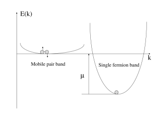
Figure 22: The Pauli exclusion principle prevents a decay of mobile bipolarons into single polarons in overdoped cuprates because all states below the Fermi level $\mu$ are occupied.

Such a system represents a mixture of mobile 2e-charged bosons and e-charged degenerate fermions, first considered by us before the discovery ale3 , somewhat similar to neutral He³-He⁴ mixtures. While the normal state kinetic properties are dominated by a lighter polaronic Fermi liquid, the superconducting state is the Bose-Einstein condensate (BEC) of heavier bipolarons in the mixture. As we discuss in the remaining part, it is valid even in the extreme case of intrinsically immobile bipolarons, if they are hybridized with mobile polarons, irrespective to the strength of the hybridization interaction.

VI.1 Mobile fermions hybridized with immobile bosons: Boson-Fermion model

As an alternative to the picture of HTS with mobile bipolarons, Figs.12,22, some authors lee ; ran ; ran0 ; kos ; lar ; dam ; dam2 ; mic proposed a so-called Boson-Fermion model (BFM), where intrinsically immobile pairs are coupled with the Fermi sea of itinerant single fermions by the hybridization interaction. Soon after Anderson and Street and Mott ander introduced localized pairs in amorphous semiconductors, such two component model of negative $U$ centers coupled with the Fermi sea of itinerant fermions was employed to study superconductivity in disordered metal-semiconductor alloys sim ; tin . When the attractive potential $U$ is large, the model is reduced to localized hard-core bosons spontaneously decaying into itinerant electrons and vice versa, different from a non-converting mixture of mobile charged bosons and fermions ale3 ; and .

This boson-fermion model (BFM) was applied more generally to describe pairing electron processes with localization-delocalization ion . The model attracted more attention in connection with high-temperature superconductors lee ; ran ; ran0 ; kos ; lar ; ale ; cris ; dam ; dam2 ; mic . In particular, Refs. dam ; dam2 claimed that 2D BFM with immobile hard-core bosons is capable to reproduce some physical properties and the phase diagram of cuprates. BFM has been also adopted for a description of superfluidity of atomic fermions scattered into bound (molecular) states chio .

Most studies of BFM below its transition into a low-temperature condensed phase applied a mean-field approximation (MFA), replacing zero-momentum boson operators by c-numbers and neglecting the boson self-energy in the density sum rule lee ; ran ; kos ; lar ; dam ; dam2 ; mic ; chio . When the bare boson energy is well above the chemical potential, the BCS ground state was found with bosons being only virtually excited lee ; ran . MFA led to a conclusion that BFM exhibits features compatible with BCS characteristics kos , and describes a crossover from the BCS-like to a local pair behavior mic . The transition was found more mean-field-like than the usual Bose condensation, i.e. characterized by a relatively small value of the fluctuation parameter $Gi$ lar .

At the same time our previous study of BFM ale beyond MFA revealed a crucial effect of the boson self-energy on the normal state boson spectral function and the transition temperature $T_{c}$. Ref.ale proved that the Cooper pairing of fermions via virtual bosonic states is impossible in any-dimensional BFM. It occurs only simultaneously with the Bose-Einstein condensation of real bosons. The origin of this simultaneous condensation lies in a softening of the boson mode at $T=T_{c}$ caused by its hybridization with fermions. The energy of zero-momentum bosons is renormalized down to zero at $T=T_{c}$, no matter how weak the boson-fermion coupling and how large the bare boson energy are ale . One can also expect that the boson self-energy should qualitatively modify the phase transition and the condensed phase of BFM below $T_{c}$.

VI.2 Absence of BCS-BEC crossover in BFM

Let us examine the phase transition and the condensed state of BFM beyond the ordinary mean-field approximation in two (2D) and three (3D)dimensions. It appears that $T_{c}=0$ K in the two-dimensional model, even in the absence of any Coulomb repulsion, and the phase transition is never a BCS-like second-order phase transition even in 3D BFM because of the complete boson softening.

The 2D BFM is defined by the Hamiltonian,

$$H = \sum_{{\bf k},\sigma=\uparrow,\downarrow}\xi_{{\bf k}}c_{{\bf k},\sigma}^{\dagger}c_{{\bf k},\sigma}+E_{0}\sum_{{\bf q}}b_{{\bf q}}^{\dagger}b_{{\bf q}}+$$

$${\rm g}N^{-1/2}\sum_{{\bf q,k}}\left(\phi_{{\bf k}}b_{{\bf q}}^{\dagger}c_{-{\bf k}+{\bf q}/2,\uparrow}c_{{\bf k}+{\bf q}/2,\downarrow}+H.c.\right),$$

where $\xi_{{\bf k}}=-2t(\cos k_{x}+\cos k_{y})-\mu$ is the 2D energy spectrum of fermions, $E_{0}\equiv\Delta_{B}-2\mu$ is the bare boson energy with respect to their chemical potential $2\mu$, ${\rm g}$ is the magnitude of the anisotropic hybridization interaction, $\phi_{{\bf k}}=\phi_{-{\bf k}}$ is the anisotropy factor, and $N$ is the number of cells. Here and further I take $\hbar=c=k_{B}=1$ and the lattice constant $a=1$. Ref. dam argued that ’superconductivity is induced in this model from the anisotropic charge-exchange interaction (${\rm g}\phi_{{\bf k}}$) between the conduction-band fermions and the immobile hard-core bosons’, and ’the on-site Coulomb repulsion competes with this pairing’ reducing the critical temperature $T_{c}$ less than by 25%. Also it has been argued dam2 , that the calculated upper critical field of the model fits well the experimental results in cuprates.

Here I show that $T_{c}=0$ K in the two-dimensional model, Eq.(131), even in the absence of any Coulomb repulsion, and the mean-field approximation is meaningless for any-dimensional BFM because of the complete boson softening. Replacing boson operators by $c$-numbers for ${\bf q}=0$ in Eq.(131) one obtains a linearized BCS-like equation for the fermion order-parameter (the gap function) $\Delta_{{\bf k}}$,

$$\Delta_{{\bf k}}=\frac{{\rm\tilde{g}}^{2}\phi_{{\bf k}}}{E_{0}N}\sum_{{\bf k}^{\prime}}\phi_{{\bf k}^{\prime}}{\frac{\Delta_{{\bf k}^{\prime}}\tanh(\xi_{{\bf k}^{\prime}}/2T)}{{2\xi_{{\bf k}^{\prime}}}},}$$ (136)

with the coupling constant ${\rm\tilde{g}}^{2}={\rm g}^{2}(1-2n^{B})$, renormalized by the hard-core effects. Using a two-particle fermion vertex part in the Cooper channel one can prove that this equation is perfectly correct even beyond the conventional non-crossing approximation ale . The problem with MFA does not stem from this BSC-like equation, but from an incorrect definition of the bare boson energy with respect to the chemical potential, $E_{0}(T)$. This energy is determined by the atomic density of bosons ($n_{b}$) as (Eq.(9) in Ref. dam )

$$\tanh\frac{E_{0}}{2T}=1-2n_{b}.$$ (137)

While Eq.(132) is perfectly correct, Eq.(133) is incorrect because the boson self-energy $\Sigma_{b}({\bf q},\Omega)$ due to the same hybridization interaction is missing. At first sight dam the self-energy is small in comparison to the kinetic energy of fermions, if ${\rm g}$ is small. However $\Sigma_{b}(0,0)$ diverges logarithmical at zero temperature ale , no matter how week the interaction is. Therefore it should be kept in the density sum-rule, Eq.(133). Introducing the boson Green’s function

$$D({\bf q},\Omega)=\frac{1-2n_{b}}{i\Omega-E_{0}-\Sigma_{b}({\bf q},\Omega)}$$ (138)

one must replace incorrect Eq.(133) by

$$-{\frac{T}{{N}}}\sum_{{\bf q},n}e^{i\Omega\tau}D({\bf q},\Omega)=n_{b},$$ (139)

where $\tau=+0$, and $\Omega=2\pi Tn$ ($n=0,\pm 1,\pm 2...$).

The divergent (cooperon) contribution to $\Sigma_{b}({\bf q},\Omega)$ is given by ale ,

$$\Sigma_{b}({\bf q},\Omega)=-\frac{{\rm\tilde{g}}^{2}}{2N}\sum_{{\bf k}}\phi_{{\bf k}}^{2}\times$$ (140)

$$\frac{\tanh[\xi_{{\bf k-q}/2}/(2T)]+\tanh[\xi_{{\bf k+q}/2}/(2T)]}{\xi_{{\bf k-q}/2}+\xi_{{\bf k+q}/2}-i\Omega},$$

so that one obtains

$$\Sigma_{b}({\bf q},0)=\Sigma_{b}(0,0)+\frac{q^{2}}{2M^{\ast}}+{\cal O}(q^{4})$$ (141)

for small ${\bf q}$ and any anisotropy factor compatible with the point-group symmetry of the cuprates. Here $M^{\ast}$ is the boson mass, calculated analytically in Ref.ale for the isotropic exchange interaction and parabolic fermion band dispersion (see also Ref.cris ). The BCS-like equation (132) has a nontrivial solution for $\Delta_{{\bf k}}$ at $T=T_{c}$, if

$$E_{0}=-\Sigma_{b}(0,0).$$ (142)

Substituting Eqs.(137,138) into the sum-rule, Eq.(135), one obtains a logarithmical divergent integral with respect to ${\bf q}$, and

$$T_{c}=\frac{const}{\int_{0}dq/q}=0.$$ (143)

The devastating result, Eq.(139) is a direct consequence of the well-known theorem, which states that BEC is impossible in 2D. One may erroneously believe that MFA results dam ; dam2 are still applied in three-dimensions, where BEC is possible. However, increasing dimensionality does not make MFA a meaningful approximation for the boson-fermion model. This approximation leads to a conclusion that a BCS-like superconducting state occurs below the critical temperature $T_{c}\simeq\mu\exp\left(-{E_{0}/z_{c}}\right)$ via fermion pairs being virtually excited into $unoccupied$ bosonic states lee ; ran . Here $z_{c}=\tilde{g}^{2}N(0)$ and $N(0)$ is the density of states (DOS) in the fermionic band near the Fermi level $\mu$. However, the Cooper pairing of fermions is impossible via virtual unoccupied bosonic states also in 3D BFM. Indeed, Eqs.(132,138) do not depend on the dimensionality, so that the analytical continuation of Eq.(132) to real frequencies $\omega$ yields the partial boson DOS as $\rho(\omega)=(1-2n_{b})\delta(\omega)$ at $T=T_{c}$ and ${\bf q}=0$ in any-dimensional BFM. The Cooper pairing may occur only simultaneously with the Bose-Einstein condensation of real bosons in the exact theory of 3D BFM ale . The origin of the simultaneous condensation of the fermionic and bosonic fields in 3D BFM lies in the softening of the boson mode at $T=T_{c}$ caused by its hybridization with fermions.

Taking into account the boson damping and dispersion shows that the boson spectrum significantly changes for all momenta. Continuing the self-energy, Eq.(136) to real frequencies yields the damping (i.e. the imaginary part of the self-energy) as ale

$$\gamma({\bf q},\omega)={\pi z_{c}\over{4q\xi}}\ln\left[{\cosh(q\xi+\omega/(4T_{c}))\over{\cosh(-q\xi+\omega/(4T_{c}))}}\right],$$ (144)

where $\xi=v_{F}/(4T_{c})$ is a coherence length, and $v_{F}$ is the Fermi velocity. The damping is significant when $q\xi<<1$. In this region $\gamma({\bf q},\omega)=\omega\pi z_{c}/(8T_{c})$ is comparable or even larger than the boson energy $\omega$. Hence bosons look like overdamped diffusive modes, rather than quasiparticles in the long-wave limit ale ; cris , contrary to the erroneous conclusion of Ref.ran0 , that there is ’the onset of coherent free-particle-like motion of the bosons’ in this limit. Only outside the long-wave region, the damping becomes small. Indeed, using Eq.(138) one obtains $\gamma({\bf q},\omega)=\omega\pi z_{c}/(2qv_{F})<<\omega$, so that bosons at $q>>1/\xi$ are well defined quasiparticles with a logarithmic dispersion, $\omega(q)=z_{c}\ln(q\xi)$ ale . Hence the boson energy disperses over the whole energy interval from zero up to $E_{0}$.

The main mathematical problem with MFA in 3D also stems from the density sum rule, Eq.(135) which determines the chemical potential of the system and consequently the bare boson energy $E_{0}(T)$ as a function of temperature. In the framework of MFA one takes the bare boson energy in Eq.(132) as a temperature independent parameter, $E_{0}=\tilde{g}^{2}N(0)\ln(\mu/T_{c})$ lar , or determines it from the conservation of the total number of particles neglecting the boson self-energy, Eq.(133) ran ; dam ; mic ; chio . Then Eq.(132) looks like the conventional linearized Ginzburg-Landau-Gor’kov equation gor2 with a negative coefficient $\alpha\propto T-T_{c}$ at $T<T_{c}$ in the linear term. Then one concludes that the phase transition is almost the conventional BCS-like transition, at least at $E_{0}\gg T_{c}$ lee ; ran ; lar . These findings are mathematically and physically erroneous. Indeed, the term of the sum in Eq.(135) with $\Omega_{n}=0$ is given by the integral

$$T\int{d{\bf q}\over{2\pi^{3}}}{1\over{E_{0}+\Sigma_{b}({\bf q},0)}}.$$ (145)

The integral converges, if and only if $E_{0}\geq-\Sigma_{b}(0,0)$. In fact,

$$E_{0}+\Sigma_{b}(0,0)=0$$ (146)

is strictly zero in the Bose-condensed state, because $\mu_{b}=-[E_{0}+\Sigma_{b}(0,0)]$ corresponds to the boson chemical potential relative to the lower edge of the boson energy spectrum. More generally, $\mu_{b}=0$ corresponds to the appearance of the Bogoliubov-Goldstone mode due to a broken symmetry below $T_{c}$. This exact result makes the BSC equation (132) simply an identity with $\alpha(T)\equiv 0$ at any temperature below $T_{c}$. On the other hand, MFA violates the density sum-rule, predicting the wrong negative $\alpha(T)$ below $T_{c}$. Since $\alpha(T)=0$, one may expect that the conventional upper critical field, $H_{c2}(T)$ is zero in BFM. To determine $H_{c2}(T)$ and explore the condensed phase of 3D BFM, one can apply the Gor’kov formalism gor2 , as described below.

VI.3 Normal and anomalous Green’s functions of 3D BFM: pairing of bosons

Let us now explore a simplified version of 3D BFM in an external magnetic field ${\bf B=\nabla\times A}$ neglecting the hard-core effects alepair ,

$$H = \int d{\bf r}\sum_{s}\psi_{s}^{\dagger}({\bf r})\hat{h}({\bf r})\psi_{s}({\bf r})+g[\phi({\bf r})\psi_{\uparrow}^{\dagger}({\bf r})\psi_{\downarrow}^{\dagger}({\bf r})+H.c.]$$ (147)

$$+ E_{0}\phi^{\dagger}({\bf r})\phi({\bf r}),$$

where $\psi_{s}({\bf r})$ and $\phi({\bf r})$ are fermionic and bosonic fields, $s=\uparrow,\downarrow$ is the spin, $\hat{h}({\bf r)=}-[\nabla+ie{\bf A(r)]}^{2}/(2m)-\mu$ is the fermion kinetic energy operator. Here the volume of the system is taken as $V=1$.

The Matsubara field operators, $Q=\exp(H\tau)Q({\bf r)}\exp(-H\tau),\bar{Q}=\exp(H\tau)Q^{\dagger}({\bf r)}\exp(-H\tau)$ ($Q\equiv\psi_{s},\phi$) evolve with the imaginary time $-1/T\leq\tau\leq 1/T$ as

$$-\frac{\partial\psi_{\uparrow}({\bf r},\tau)}{\partial\tau} = \hat{h}({\bf r)}\psi_{\uparrow}({\bf r},\tau)+g\phi({\bf r},\tau)\bar{\psi}_{\downarrow}({\bf r,}\tau),$$ (148)

$$\frac{\partial\bar{\psi}_{\downarrow}({\bf r,}\tau)}{\partial\tau} = \hat{h}^{\ast}({\bf r)}\bar{\psi}_{\downarrow}({\bf r,}\tau)-g\bar{\phi}({\bf r},\tau)\psi_{\uparrow}({\bf r,}\tau),$$ (149)

$$-\frac{\partial\phi({\bf r,}\tau)}{\partial\tau} = E_{0}\phi({\bf r,}\tau)+g\psi_{\downarrow}({\bf r,}\tau)\psi_{\uparrow}({\bf r,}\tau).$$ (150)

The theory of the condensed state can be formulated with the normal and anomalous fermion GFs gor2 , ${\cal G}({\bf r,r}^{\prime},\tau)=-\langle T_{\tau}\psi_{s}({\bf r},\tau)\bar{\psi}_{s}({\bf r}^{\prime}{\bf,}0)\rangle$, ${\cal F}^{+}({\bf r,r}^{\prime},\tau)=\langle T_{\tau}\bar{\psi}_{\downarrow}({\bf r,}\tau)\bar{\psi}_{\uparrow}({\bf r}^{\prime},0)\rangle$, respectively, where the operation $T_{\tau}$ performs the time ordering. Fermionic and bosonic fields condense simultaneously ale . Following Bogoliubov bog the bosonic condensate is described by separating a large matrix element $\phi_{0}({\bf r})$ in $\phi({\bf r},\tau)$ as a number, while the remaining part $\tilde{\phi}({\bf r},\tau)$ describes a supracondensate field, $\phi({\bf r},\tau)=\phi_{0}({\bf r})+\tilde{\phi}({\bf r},\tau)$. Then using Eq.(146) one obtains

$$g\phi_{0}({\bf r})=\Delta({\bf r})\equiv-{g^{2}\over{E_{0}}}{\cal F}({\bf r,r},0+),$$ (151)

where ${\cal F}({\bf r,r}^{\prime},\tau)=\langle T_{\tau}\psi_{\downarrow}({\bf r,}\tau)\psi_{\uparrow}({\bf r}^{\prime},0)\rangle$. The equations for GFs are obtained by using Eqs. (144-146) and the diagrammatic technique abr in the framework of the non-crossing approximation ref , as shown in Fig.23 and Fig.24.

An important novel feature of BFM is a pairing of supracondensate bosons, caused by their hybridization with the fermionic condensate, as follows from the last diagram in Fig.24. Hence, one has to introduce an anomalous supracondensate boson GF, ${\cal B}^{+}({\bf r,r}^{\prime},\tau)=\langle T_{\tau}\bar{\tilde{\phi}}({\bf r,}\tau)\bar{\tilde{\phi}}({\bf r}^{\prime},0)\rangle$ along with the normal boson GF, ${\cal D}({\bf r,r}^{\prime},\tau)=-\langle T_{\tau}\tilde{\phi}({\bf r},\tau)\bar{\tilde{\phi}}({\bf r}^{\prime}{\bf,}0)\rangle$.

Figure 23: Diagrams for the normal and anomalous fermion GFs. Zig-zag arrows represent the single-particle Bose condensate $\phi_{0}$, dotted lines are the boson GFs, solid lines are the fermion GFs. Vertex (dot) corresponds to the hybridization interaction.

The diagrams, Fig.23 and Fig.24, are transformed into analytical equations for the time Fourier-components of the fermion GFs with the Matsubara frequencies $\omega=\pi T(2n+1)$ ($n=0,\pm 1,\pm 2,...$) as

$$[i\omega-\hat{h}({\bf r)}]{\cal G}_{\omega}({\bf r,r}^{\prime})=\delta({\bf r-r}^{\prime})-\Delta({\bf r)}{\cal F}_{\omega}^{+}({\bf r,r}^{\prime})$$ (152)

$$- g^{2}T\sum_{\omega^{\prime}}\int d{\bf x}{\cal G}_{-\omega^{\prime}}({\bf x,r}){\cal D}_{\omega-\omega^{\prime}}({\bf r,x}){\cal G}_{\omega}({\bf x,r}^{\prime})$$ (153)

$$- g^{2}T\sum_{\omega^{\prime}}\int d{\bf x}{\cal F}^{+}_{\omega^{\prime}}({\bf r,x}){\cal B}_{\omega+\omega^{\prime}}({\bf r,x}){\cal F}^{+}_{\omega}({\bf x,r^{\prime}}),$$ (154)

$$[-i\omega-\hat{h}^{\ast}({\bf r)}]{\cal F}^{+}_{\omega}({\bf r,r}^{\prime})=\Delta^{\ast}({\bf r)}{\cal G}_{\omega}({\bf r,r}^{\prime})$$ (155)

$$- g^{2}T\sum_{\omega^{\prime}}\int d{\bf x}{\cal G}_{\omega^{\prime}}({\bf r,x}){\cal D}_{\omega^{\prime}-\omega}({\bf x,r}){\cal F}^{+}_{\omega}({\bf x,r}^{\prime})$$

$$+ g^{2}T\sum_{\omega^{\prime}}\int d{\bf x}{\cal F}_{-\omega^{\prime}}({\bf r,x}){\cal B}^{+}_{-\omega-\omega^{\prime}}({\bf r,x}){\cal G}_{\omega}({\bf x,r^{\prime}}),$$

and

$$(i\Omega-E_{0}){\cal D}_{\Omega}({\bf r,r}^{\prime})=\delta({\bf r-r}^{\prime})$$ (157)

$$- g^{2}T\sum_{\omega^{\prime}}\int d{\bf x}{\cal G}_{\omega^{\prime}}({\bf r,x}){\cal G}_{\Omega-\omega^{\prime}}({\bf r,x}){\cal D}_{\Omega}({\bf x,r}^{\prime})$$ (158)

$$- g^{2}T\sum_{\omega^{\prime}}\int d{\bf x}{\cal F}_{\omega^{\prime}}({\bf r,x}){\cal F}_{\Omega-\omega^{\prime}}({\bf r,x}){\cal B}^{+}_{\Omega}({\bf x,r}^{\prime}),$$ (159)

$$(-i\Omega-E_{0}){\cal B}^{+}_{\Omega}({\bf r,r}^{\prime})=$$

$$g^{2}T\sum_{\omega^{\prime}}\int d{\bf x}{\cal F}_{-\omega^{\prime}}^{+}({\bf r,x}){\cal F}_{-\Omega+\omega^{\prime}}^{+}({\bf r,x}){\cal D}_{\Omega}({\bf x,r^{\prime}})$$

$$- g^{2}T\sum_{\omega^{\prime}}\int d{\bf x}{\cal G}_{-\omega^{\prime}}({\bf x,r}){\cal G}_{\omega^{\prime}-\Omega}({\bf x,r}){\cal B}^{+}_{\Omega}({\bf x,r}^{\prime}).$$

for the boson GFs with ${\cal B}({\bf r,r}^{\prime},\tau)=\langle T_{\tau}\tilde{\phi}({\bf r,}\tau)\tilde{\phi}({\bf r}^{\prime},0)\rangle$.

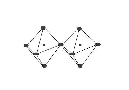
Figure 24: Diagrams for the supracondensate boson GFs. The Cooper-pairing of fermions leads to the Cooper-pair-like boson condensate, described by the boson anomalous GF, ${\cal B}^{+}$.

VI.4 Gor’kov expansion

These equations can be formally solved in the homogeneous case without the external field, ${\bf A}=0$. Transforming into the momentum space yields GFs’ time-space Fourier components as

$${\cal G}({\bf k},\omega) =- {\frac{i\tilde{\omega}^{\ast}+\xi_{\bf k}}{|i\tilde{\omega}-\xi_{\bf k}|^{2}+|\tilde{\Delta}({\bf k},\omega)|^{2}}},$$ (162)

$${\cal F}^{+}({\bf k},\omega) = {\frac{\tilde{\Delta}^{\ast}({\bf k},\omega)}{|i\tilde{\omega}-\xi_{\bf k}|^{2}+|\tilde{\Delta}({\bf k},\omega)|^{2}}},$$ (163)

and

$${\cal D}({\bf q},\omega) = -{\frac{i\tilde{\Omega}^{\ast}+E_{0}}{|i\tilde{\Omega}-E_{0}|^{2}+|\Gamma({\bf q},\Omega)|^{2}}},$$ (164)

$${\cal B}^{+}({\bf q},\omega) = {\frac{\Gamma^{\ast}({\bf q},\Omega)}{|i\tilde{\Omega}-E_{0}|^{2}+|\Gamma({\bf q},\Omega)|^{2}}},$$ (165)

where $\tilde{\omega}\equiv\omega+i\Sigma_{f}({\bf k},\omega)$, $\tilde{\Omega}\equiv\Omega+i\Sigma_{b}({\bf q},\Omega)$, and $\xi_{\bf k}=k^{2}/(2m)-\mu$. The fermionic order parameter, renormalized with respect to the mean-field $\Delta$ due to the formation of the boson-pair condensate, is given by

$$\tilde{\Delta}({\bf k},\omega)=\Delta+g^{2}T\sum_{\omega^{\prime}}\int{d{\bf q}\over{2\pi^{3}}}{\cal F}^{+}({\bf k}-{\bf q},\omega^{\prime}){\cal B}({\bf q},\omega+\omega^{\prime}),$$ (166)

and the boson-pair order parameter, generated by the hybridization with the fermion Cooper pairs, is

$$\Gamma({\bf q},\Omega)=g^{2}T\sum_{\omega^{\prime}}\int{d{\bf k}\over{2\pi^{3}}}{\cal F}({\bf k},\omega^{\prime}){\cal F}({\bf q}-{\bf k},\Omega-\omega^{\prime}).$$ (167)

Hence, there are three coupled condensates in the model described by the off-diagonal fields $g\phi_{0}$, $\tilde{\Delta}$, and $\Gamma$, rather than two, as in MFA. At low temperatures all of them have about the same magnitude, as the fermion and boson self-energies,

$$\Sigma_{f}({\bf k},\omega)=-g^{2}T\sum_{\omega^{\prime}}\int{d{\bf q}\over{2\pi^{3}}}{\cal G}({\bf q}-{\bf k},-\omega^{\prime}){\cal D}({\bf q},\omega-\omega^{\prime}),$$ (168)

$$\Sigma_{b}({\bf q},\Omega)=-g^{2}T\sum_{\omega^{\prime}}\int{d{\bf q}\over{2\pi^{3}}}{\cal G}({\bf k},\omega^{\prime}){\cal G}({\bf q}-{\bf k},\Omega-\omega^{\prime}),$$ (169)

respectively.

On the other hand, when the temperature is close to $T_{c}$ (i.e. $T_{c}-T\ll T_{c}$), the boson pair condensate is weak compared with the single-particle boson and the Cooper pair condensates. In this temperature range $\Gamma$, Eq.(155) is of the second order in $\Delta$, $\Gamma\propto\Delta^{2}$, so that the anomalous boson GF can be neglected, since $\Delta$ is small. The fermion self-energy, Eq.(156) is a regular function of $\omega$ and ${\bf k}$, so it can be absorbed in the renormalized fermion band dispersion. Then the fermion normal and anomalous GFs, Eqs.(150,151) look like the familiar GFs of the BCS theory, and one can apply the Gor’kov expansion gor2 in powers of $\Delta({\bf r)}$ to describe the condensed phase of BFM in the magnetic field near the transition. Using Eq.(147) one obtains to the terms linear in $\Delta$

$$\Delta^{\ast}({\bf r)}={g^{2}\over{E_{0}}}T\sum_{\omega_{n}}\int d{\bf x}{\cal G}_{-\omega_{n}}^{(n)}({\bf x,r})\Delta^{\ast}({\bf x)}{\cal G}_{\omega_{n}}^{(n)}({\bf x,r}).$$ (170)

The spatial variations of the vector potential are small near the transition. If ${\bf A}({\bf r})$ varies slowly, the normal state GF, ${\cal G}_{\omega}^{(n)}({\bf r,r}^{\prime})$ differs from the zero-field normal state GF, ${\cal G}_{\omega}^{(0)}(\bf{r-r^{\prime}})$ only by a phase gor2 ${\cal G}_{\omega}^{(n)}({\bf r,r}^{\prime})=\exp[-ie{\bf A(r)}\cdot(\bf{r-r}^{\prime})]{\cal G}_{\omega}^{(0)}(\bf{r-r}^{\prime})$. Expanding all quantities near the point ${\bf x=r}$ in Eq.(158) up to the second order in ${\bf x-r}$ inclusive, one obtains the linearized equation for the fermionic order parameter as

$$\gamma[\nabla-2ie{\bf A(r)]}^{2}\Delta({\bf r})=\alpha\Delta({\bf r}),$$ (171)

where

$$\alpha=1+{\Sigma_{b}(0,0)\over{E_{0}}}\approx 1-{g^{2}N(0)\over{E_{0}}}\ln{\mu\over{T}},$$ (172)

and $\gamma\approx 7\zeta(3)v_{F}^{2}g^{2}N(0)/(48\pi^{2}T^{2}E_{0})$.

The coefficient $\alpha(T)$ disappears in Eq.(159), since $E_{0}=-\Sigma_{b}(0,0)$ at and below $T_{c}$. It means that the phase transition is never a BCS-like second-order phase transition even at large $E_{0}$ and small $g$. In fact, the transition is driven by the Bose-Einstein condensation of real bosons with ${\bf q}=0$, which occur due to the complete softening of their spectrum at $T_{c}$. Remarkably, the conventional upper critical field, determined as the field, where a non-trivial solution of the linearized Gor’kov equation (159) occurs, is zero in BFM, $H_{c2}(T)=0$. It is not a finite $H_{c2}(T)$ found in Ref. dam using MFA. The qualitative failure of MFA might be rather unexpected, if one believes that bosons in Eq.(131) play the same role as phonons in the BCS superconductor. This is not the case for two reasons. The first one is the density sum-rule, Eq.(135), for bosons which is not applied to phonons. The second being that the boson self-energy is given by the divergent (at $T=0$) Cooperon diagram, while the self-energy of phonons is finite at small coupling.

Even at temperatures well below $T_{c}$ the condensed state is fundamentally different from the MFA ground state, because of the pairing of bosons. The latter is similar to the Cooper-like pairing of supracondensate ${}^{4}He$ atoms pas , proposed as an explanation of the small density of the single-particle Bose condensate in superfluid Helium-4. The pair-boson condensate should significantly modify the thermodynamic properties of the condensed BFM compared with the MFA predictions. Hence the common wisdom that at weak coupling the boson-fermion model is adequately described by the BCS theory is negated by our analysis beyond MFA. There is no BCS-BEC crossover in BFM, and the phase transition is of the BEC-type at any parameters.

VII Conclusion

Here I have argued that attractive electron correlations, prerequisite to HTS, are caused by an almost unretarded electron-phonon interaction sufficient to overcome the direct Coulomb repulsion in cuprates. Low energy physics of high-temperature superconductors is that of lattice polarons and of real-space hole pairs dressed by phonons, i.e. mobile lattice bipolarons. Single polarons are thermal excitations in underdoped cuprates, but they could be degenerate in the boson-fermion mixture in overdoped cuprates. The superconducting state is the Bose-Einstein 3D condensate of bipolarons at any doping including the overdoped domain, irrespective to a possible hybridization of single polarons and bipolarons. Our multi-polaron approach to the HTS problem accounts for many normal state properties of superconducting cuprates including the temperature-dependent spin susceptibility, nonlinear in-plane and thermally activated out-of-plane resistivities, the temperature-dependent Hall effect, the Nernst signal and diamagnetism above $T_{c}$, spin and charge pseudogaps. It provides a parameter-free fit of experimental $T_{c}$ and describes isotope effects, specific heat anomalies, resistive upper critical fields, and the symmetry and space modulations of the order parameter.

I thank A.M. Bratkovsky, C.J. Dent, P.P. Edwards, J.P. Hague, V.V. Kabanov, P.E. Kornilovitch, W.Y. Liang, J.H. Samson, P.E. Spencer, and V.N. Zavaritsky for a long-standing collaboration and valuable discussions. I highly appreciate enlightening discussions with A.F. Andreev, I. Bozovic, L.P. Gor’kov, J.E. Hirsch, A.P. Levanyuk, R. Micnas, D. Mihailovic, and S. Robaszkiewicz. The work was supported by EPSRC (UK) (grant EP/C518365/1), the Leverhulme Trust (UK), the Royal Society, and by NATO.

REFERENCES

REFERENCES

- (1) J. Bardeen, L.N. Cooper, and J.R. Schrieffer, Phys. Rev 108, 1175 (1957).
- (2) G.M. Eliashberg, Zh. Eksp. Teor. Fiz. 38, 966 (1960); 39, 1437 (1960) [Sov. Phys. JETP 11, 696; 12, 1000 (1960)].
- (3) A.S. Alexandrov, Theory of Superconductivity: From Weak to Strong Coupling (IoP Publishing, Bristol and Philadelphia, 2003).
- (4) N.F.Mott, Metal-Insulator Transitions, 2nd ed (Taylor&Francis, London 1990).
- (5) M. Merz, N. Nucker, P. Schweiss, S. Schuppler, C.T. Chen, V. Chakarian, J. Freeland, Y.U. Idzerda, M. Klaser, G. Muller-Vogt, and Th. Wolf, Phys. Rev. Lett. 80, 5192 (1998).
- (6) V.I. Anisimov, F. Aryasetiawamn, and A.I. Lichtenstein, J. Phys.: Condens. Matter 9, 767 (1997).
- (7) S.G. Ovchinnikov, V.A. Gavrichkov, and M.M. Korshunov, Physica B359, 1168 (2005)
- (8) R.B. Laughlin, cond-mat/0209269; B.A. Bernevig, R.B. Laughlin, and D.I. Santiago, Phys. Rev. Lett. 91, 147003 (2003).
- (9) For a comprehensive review of the Hubbard and models see N.M. Plakida, in Lectures on the Physics of Highly Correlated Electron Systems , 121 (ed. F. Mancini, American Institute of Physics, Melville NY, 2001).
- (10) A.S. Alexandrov and A.M. Bratkovsky, Phys. Rev. Lett. 84, 2043 (2000).
- (11) J.H. Kim, B.J. Feenstra, H.S. Somal, D. van der Marel, W.Y. Lee, A.M. Gerrits, and A. Wittlin, Phys. Rev. B49, 13065 (1994).
- (12) G. Zhao and D. E. Morris Phys. Rev. B 51, 16487 (1995); G.-M. Zhao, M. B. Hunt, H. Keller, and K. A. Müller, Nature (London) 385, 236 (1997); R. Khasanov, D. G. Eshchenko, H. Luetkens, E. Morenzoni, T. Prokscha, A. Suter, N. Garifianov, M. Mali, J. Roos, K. Conder, and H. Keller Phys. Rev. Lett. 92, 057602 (2004).
- (13) A. Lanzara, P.V. Bogdanov, X.J. Zhou, S.A. Kellar, D.L. Feng, E.D. Lu, T. Yoshida, H. Eisaki, A. Fujimori,K. Kishio, J.I. Shimoyana, T. Noda, S. Uchida, Z. Hussain and Z.X. Shen, Nature (London) 412, 510 (2001); G-H. Gweon, T. Sasagawa, S.Y. Zhou, J. Craf, H. Takagi, D.-H. Lee, and A. Lanzara, Nature (London) 430, 187 (2004); X. J. Zhou, J. Shi, T. Yoshida, T. Cuk, W. L. Yang, V. Brouet, J. Nakamura, N. Mannella, S. Komiya, Y. Ando, F. Zhou, W. X. Ti, J. W. Xiong, Z. X. Zhao, T. Sasagawa, T. Kakeshita, H. Eisaki, S. Uchida, A. Fujimori, Z.-Y. Zhang, E. W. Plummer, R. B. Laughlin, Z. Hussain, and Z.-X. Shen, cond-mat/0405130.
- (14) D. Mihailovic, C.M. Foster, K. Voss, and A.J. Heeger, Phys. Rev. B42, 7989 (1990).
- (15) P. Calvani, M. Capizzi, S. Lupi, P. Maselli, A. Paolone, P. Roy, S.W. Cheong, W. Sadowski, and E. Walker, Solid State Commun. 91, 113 (1994).
- (16) R. Zamboni, G. Ruani, A.J. Pal, and C. Taliani, Solid St. Commun. 70, 813 (1989).
- (17) T. Timusk, C.C. Homes, and W. Reichardt, in Anharmonic properties of High Tc cuprates (eds. D. Mihailovic, G. Ruani, E. Kaldis, and K.A. Müller, Singapore: World Scientific, p.171 (1995)).
- (18) T.R. Sendyka, W. Dmowski, and T. Egami, Phys. Rev. B51, 6747 (1995); T. Egami, J. Low Temp. Phys. 105, 791 (1996).
- (19) A.S. Alexandrov and J. Ranninger, Phys. Rev. B23 1796 (1981), ibid 24, 1164 (1981); A.S. Alexandrov, Russ. J. Phys. Chem. 57 167 (1983); A. S. Alexandrov, J. Ranninger, and S. Robaszkiewicz, Phys. Rev. B 33, 4526 (1986).
- (20) J.G. Bednorz and K.A. Müller, Z. Phys. B64, 189 (1986).
- (21) M.K. Wu, J.R. Ashburn, C.J. Torng, P.H. Hor, R.L. Meng, L. Gao, Z.J. Huang, Y.Q. Wang, and C.W. Chu, Phys. Rev. Lett. 58 , 908 (1987).
- (22) I. Bozovic, G. Logvenov, M. A. J. Verhoeven, P. Caputo, E. Goldobin, and T. H. Geballe, Nature (London) 422, 873 (2003).
- (23) A.S. Alexandrov, J. Low Temp. Phys. 87, 721 (1992).
- (24) D. Mihailovic, V.V. Kabanov, K. Zagar, and J. Demsar, Phys. Rev. B60, 6995 (1999) and references therein.
- (25) A.S. Alexandrov, V.V. Kabanov, and N.F. Mott, Phys. Rev. Lett. 77, 4796 (1996).
- (26) A.S. Alexandrov, Phys. Rev. B53, 2863 (1996)
- (27) A.S. Alexandrov and P.E. Kornilovitch, J. Phys. Cond. Matt. 14, 5337(2002)
- (28) A.B. Migdal, Zh. Eksp. Teor. Fiz. 34, 1438 (1958)[Sov. Phys. JETP 7, 996 (1958)].
- (29) A.S. Alexandrov, Europhys. Lett. 56, 92 (2001).
- (30) A.S. Alexandrov and P.E. Kornilovitch, Phys. Rev. Lett. , 807 (1999); P.E. Spencer, J.H. Samson, P.E. Kornilovitch, and A.S. Alexandrov, Phys. Rev. B71, 184319 (2005).
- (31) H. Fehske, J. Loos, and G. Wellein, Phys. Rev. B 61, 8016 (2000).
- (32) J. Bonča and S. A. Trugman, Phys. Rev. B 64, 094507 (2001).
- (33) L.D. Landau, J. Phys. (USSR) 3, 664 (1933).
- (34) S.I. Pekar, Zh. Eksp. Teor. Fiz. 16, 335 (1946).
- (35) H. Fröhlich, Adv. Phys. 3, 325 (1954).
- (36) R.P. Feynman, Phys. Rev. 97, 660 (1955).
- (37) E.I. Rashba, Opt. Spectr. 2, 75 (1957); Excitons (eds. E.I. Rashba and D.M. Struge, Nauka, Moscow (1985)).
- (38) J.T. Devreese, in Encyclopedia of Applied Physics, vol. 14, p. 383 (VCH Publishers (1996)).
- (39) S.V. Tjablikov, Zh.Eksp.Teor.Fiz 23, 381 (1952).
- (40) J. Yamashita and T. Kurosawa, J. Phys.Chem. Solids 5, 34 (1958)
- (41) G.L. Sewell, Phil. Mag. 3, 1361 (1958).
- (42) T. Holstein, Ann. Phys. 8, 325; 343 (1959). L. Friedman and T. Holstein, Ann. Phys. 21, 494 (1963); D. Emin and T. Holstein, Ann. Phys. 53, 439 (1969).
- (43) I.G. Lang and Yu. A. Firsov, Sov. Phys. JETP 16, 1301 (1962).
- (44) D.M. Eagles, Phys. Rev. 130, 1381 (1963).
- (45) J. Appel, in Solid State Physics 21(eds. F. Seitz, D. Turnbull, and H. Ehrenreich, Academic Press (1968)); Yu. A. Firsov (ed) Polarons (Nauka, Moscow, (1975)); H. Boettger and V.V. Bryksin, Hopping Conduction in Solids ( Academie-Verlag, Berlin (1985)); A.M. Stoneham, J. Chem. Soc. Farad II 85, 505 (1989); G.D. Mahan, Many Particle Physics (Plenum Press, New York (1990)); A.L. Shluger and A.M. Stoneham, J. Phys. Cond. Matt. 1, 3049 (1993); A.S. Alexandrov and N.F. Mott, Polarons and Bipolarons (World Scientific (1995)); N. Itoh and A.M. Stoneham, Materials Modification by Electronic Excitation (Cambridge University Press, Cambridge (2001)).
- (46) V.L. Vinetskii and M.Sh. Gitterman, Sov. Phys. JETP 13, 1023 (1961).
- (47) S.G. Suprun and B. Ya. Moizhes, Sov. Phys. Solid State 24, 903 (1982).
- (48) J. Adamowskii, Phys. Rev. B39, 3649 (1989).
- (49) D. Emin, Phys. Rev. Lett. 62, 1544 (1989).
- (50) F. Bassani, M. Geddo, G. Iadonisi, and D. Ninno, Phys. Rev. B43, 5296 (1991).
- (51) G. Verbist, F.M. Peeters, and J.T. Devreese, Phys. Rev. B43, 2712 (1991).
- (52) K.A. Müller, Physica Scripta T102, 39 (2002), and references therein.
- (53) P.W. Anderson, Phys. Rev. Lett. 34, 953 (1975); R.A. Street and N.F. Mott, Phys. Rev. Lett. 35, 1293 (1975).
- (54) B.K. Chakraverty, J. Phys. Lett. (Paris)40, L-99 (1979).
- (55) S. Aubry, in Polarons and Bipolarons in High-Tc Superconductors and Related Materials (eds. E.K.H. Salje, A.S. Alexandrov, and W.Y. Liang, Cambridge University Press, Cambridge) p. 271 (1995).
- (56) C.R.A. Catlow, M.S. Islam, and X. Zhang, J. Phys.: Condens. Matter 10, L49 (1998).
- (57) A.S. Alexandrov and N.F. Mott, J. Supercond (US), 7, 599 (1994).
- (58) N. Bogoliubov, J.Phys. USSR 11, 23 (1947).
- (59) A.S. Alexandrov, A.M. Bratkovsky, and N.F. Mott, Phys. Rev. Lett. 72, 1734 (1994).
- (60) A.S. Alexandrov, Physica C363, 231 (2001).
- (61) A.J. Leggett, Physica Fennica 8, 125 (1973); J Stat. Phys. 93, 927 (1998); V.N. Popov Functional Integrals and Collective Excitations (Cambridge University Press, Cambridge (1987))
- (62) L. Pietronero, S. Strässler, and C. Grimaldi, Phys. Rev. B52, 10516 (1995).
- (63) W.M. Chen, J.P. Franck, and J. Jung, Physica C341, 1875 (2000).
- (64) A.S. Alexandrov, V.N. Zavaritsky, and S. Dzhumanov, Phys. Rev. B69, 052505 (2004).
- (65) Here the polaron DOS is energy independent different from Eq.(8) in Ref.alekabmot with a one-dimensional DOS.
- (66) J.W. Loram, K.A. Mirza, and J.R. Cooper, in High Temperature Superconductivity (Research Review 1998, ed. W.Y. Liang, IRC Superconductivity, University of Cambridge, page 77) and references therein.
- (67) A.S. Alexandrov and N.F. Mott, Phys. Rev. Lett, 71, 1075 (1993).
- (68) Y. Zhang, N. P. Ong, Z.A. Xu, K. Krishana, R. Gagnon, and L. Taillefer, Phys. Rev. Lett. 84, 2219 (2000).
- (69) K.K. Lee, A.S. Alexandrov, and W.Y. Liang, Phys. Rev. Lett. 90 , 217001 (2003).
- (70) Z.A. Xu, N.P. Ong, Y. Wang, T. Kakeshita, and S. Uchida, Nature (London) 406, 486 (2000); N.P. Ong and Y. Wang, Physica C408, 11 (2004) and references therein.
- (71) C. Capan, K. Behnia, J. Hinderer, A.G.M. Jansen, W. Lang, C. Marcenat, C. Martin, and J. Flouquet, Phys. Rev. Lett. 88, 056601 (2002).
- (72) C. Capan and K. Behnia, cond-mat/0501288.
- (73) Y. Wang, L. Li, M.J. Naughton, G.D. Gu, S. Uchida, and N.P. Ong, cond-mat/0503190.
- (74) V.J. Emery and S.A. Kivelson, Nature (London), 374, 434 (1995).
- (75) V.N. Zavaritsky and A.S. Alexandrov, Phys. Rev. B71, 012502 (2005).
- (76) V.N. Zavaritsky, J. Vanacken, V.V. Moshchalkov, and A.S. Alexandrov, Eur. Phys. J. B42, 367 (2004).
- (77) B. Bucher, J. Karpinski, E. Kaldis, and P. Wachter, Physica C167 324 (1990).
- (78) A.P. Mackenzie, S.R. Julian, G.G. Lonzarich, A. Carrington, S.D. Hughes, R.S. Liu, and D.C. Sinclair, Phys. Rev. Lett. 71, 1238 (1993)
- (79) M.A. Osofsky, R.J. Soulen, A.A. Wolf, J.M. Broto, H. Rakoto, J.C. Ousset, G. Coffe, S. Askenazy, P. Pari, I. Bozovic, J.N. Eckstein, and G.F. Virshup, Phys. Rev. Lett. 71, 2315 (1993).; ibid 72, 3292 (1994).
- (80) D.D. Lawrie, J.P. Franck, J.R. Beamish, E.B. Molz, W.M. Chen, and M.J. Graf, J. Low Temp. Phys. 107, 491 (1997).
- (81) V.F. Gantmakher, G.E. Tsydynzhapov, L.P. Kozeeva, and A.N. Lavrov, Zh. Eksp. Teor. Fiz. 88 148 (1999).
- (82) A.S. Alexandrov, V.N. Zavaritsky, W.Y. Liang, and P.L. Nevsky, Phys. Rev. Lett. 76 983 (1996).
- (83) J. Hofer, J. Karpinski, M. Willemin, G.I. Meijer, E.M. Kopnin, R. Molinski, H. Schwer, C. Rossel, and H. Keller, Physica C 297, 103 (1998).
- (84) V.N. Zverev and D.V. Shovkun, JETP Lett. 72, 73 (2000).
- (85) A.S. Alexandrov and V.N. Zavaritsky, Phys. Rev. Lett. 93, 217002 (2004).
- (86) A.S. Alexandrov, cond-mat/0507268.
- (87) A. Ettingshausen and W. Nernst, Wied. Ann. 29,343 (1886).
- (88) S.R. Elliot, Physics of amorphous materials, pp. 222-225 (Longman, New York, 1983).
- (89) N.F. Mott, E.A. Davis, and R.A. Street, Phil Mag. 32, 961 (1975).
- (90) E.H. Sondheimer, Proc. Roy. Soc. 193, 484 (1948).
- (91) L. Friedman, J. Non-Cryst.Sol. 6, 329 (1971); T. Holstein, Phil Mag. 27, 225 (1973); D. Emin, Phil Mag. 35, 1189 (1977).
- (92) A.S. Alexandrov and R.T. Giles, J. Phys.: Cond. Matt. 9, 9921 (1997).
- (93) M. Cutler and N.F. Mott, Phys. Rev. 181, 1336 (1969).
- (94) A.S. Alexandrov, Phys. Lett. A236, 132 (1997).
- (95) J. Vanacken, personal communication (2004).
- (96) C.Y. Chen, E.C. Branlund, C.S. Bae, K. Yang, M.A. Kastner, A. Cassanho, and R.J. Birgeneau, Phys. Rev. B51, 3671 (1995).
- (97) C. Erginsoy, Phys. Rev. 79, 1013 (1950).
- (98) C. Bergemann, A.W. Tyler, A.P. Mackenzie, J. R. Cooper, S.R. Julian, and D.E. Farrel, Phys. Rev. B 57, 14387 (1998).
- (99) A. Junod, J-Y. Genouda, G. Trisconea, and T. Schneider, Physica C 294, 115 (1998).
- (100) M. J. Naughton, Phys. Rev. B61, 1605 (2000).
- (101) J. Hofer, T. Schneider, J.M. Singer, M. Willemin, H. Keller, T. Sasagawa, K. Kishio, K. Conder, and J. Karpinski, Phys. Rev. B 62, 631 (2000).
- (102) I. Iguchi, A. Sugimoto, and H. Sato, J. Low Temp. Phys. 131, 451 (2003).
- (103) J.L. Tallon, J.R. Cooper, S.H. Naqib, and J.W. Loram, cond-mat/0410568.
- (104) C.J. Dent, A.S. Alexandrov, and V.V. Kabanov, Physica C341-348, 153 (2000).
- (105) A.S. Alexandrov, Doctoral Thesis MEPHI (Moscow, 1984); Phys. Rev. B48, 10571 (1993).
- (106) V.N. Zavaritsky, V.V. Kabanov and A.S. Alexandrov, Europhys. Lett. 60, 127 (2002)
- (107) M.R. Schafroth, Phys. Rev. 100, 463 (1955).
- (108) T. Machi, I. Tomeno, T. Miyatake, and S. Tanaka, Physica C173, 32 (1991).
- (109) J. Rossat-Mignod, L.P. Regnault, P. Bourges, C. Vettier, P. Burlet, and J.Y. Henry, Physica Scripta 45 74 (1992).
- (110) H.A. Mook, M. Yethiraj, G. Aeppli, T.E. Mason, and T. Armstrong, Phys. Rev. Lett. 70, 3490 (1993).
- (111) X.H. Chen, M. Yu, K.Q. Ruan, S.Y. Li, Z. Gui, G.C. Zhang, and L.Z. Cao, Phys. Rev. B58, 14219 (1998).
- (112) K.A. Müller, Guo-meng Zhao, K. Conder, and H. Keller, J. Phys. Cond. Matt. 10, L291 (1998).
- (113) A.S. Alexandrov, Phys. Rev. Lett. 82, 2620 (1999); A.S. Alexandrov and V.V. Kabanov, Phys. Rev. B59 13628 (1999).
- (114) A.S. Alexandrov(Aleksandrov) and V.V. Kabanov, Fiz. Tverd. Tela 28, 1129 (1986) [ Soviet Phys. Solid St. 28, 631 (1986)].
- (115) Y.J. Uemura, Polarons and Bipolarons in High-Tc Superconductors and Related Materials (eds. E.K.H. Salje, A.S. Alexandrov, and W.Y. Liang, Cambridge University Press, Cambridge) p. 453 (1995).
- (116) B.J. Alder and D. Peters,1989 Europhys. Lett. 10, 1 (1989).
- (117) V.L. Pokrovsky, Pis’ma Zh. Teor. Fiz. 47, 539, (1988).
- (118) T. Schneider and J.M. Singer, Phase Transition Approach To High Temperature Superconductivity ( Imperial College Press, London (2000)).
- (119) D. M. Eagles, Phys. Rev. 186, 456 (1969).
- (120) A.J. Legget, J. Phys. (Paris) 41, C7 (1980).
- (121) P. Nozieres P and S. Schmitt-Rink, J.Low Temp. Phys. 59, 195 (1985).
- (122) R. Micnas and T. Kostyrko, in Recent developments in High Temperature Superconductivity (eds. P.W. Klamut and M. Kazimierski, Springer Verlag, Berlin (1995)), p. 221 and references therein.
- (123) B.L. Gyorffy, J.B. Staunton, and G.M. Stocks, Phys. Rev. B44, 5190 (1991); E.V. Gorbar, V.M. Loktev, and S.G. Sharapov, Physica C257, 355 (1996); F. Pistolesi and G.C. Strinati, Phys. Rev. B53 , 15168 (1996); M. Marini, F. Pistolesi, and G.C. Strinati, Eur. Phys. J. B1, 158 (1998); J Maly, K. Levin, and D.Z. Liu, Phys. Rev. B54, 15657 (1996);
- (124) A.S. Alexandrov and S.G. Rubin, 1993 Phys. Rev. B47, 5141 (1993).
- (125) N. Tiverdi and M. Randeria, Phys. Rev. Lett.75, 312 (1995); J.M. Singer, M.H. Pedersen, and T. Schneider, 1995 Physica B230, 955 (1995).
- (126) S. Schmitt Rink, C.M. Varma, and A.E. Ruckenstein, Phys. Rev. Lett. 63, 445 (1989).
- (127) S.V. Traven, Phys. Rev. B51, 3242 (1994).
- (128) M.K. Crawford, W.E. Farneth, E.M. McCarron III, R.L. Harlow, and A.H. Moudden, Science 250, 1309 (1990).
- (129) H.J. Bornemann, D.E. Morris, H.B. Liu, A.P. Sinha, P. Narwankar, and M. Chandrachood, Physica C185-189, 1359 (1991).
- (130) J.P. Franck, J. Jung, G.J. Salomons, W.A. Miner, M.A.K. Mohamed, J. Chrzanowski, S. Gygax, J.C. Irwin, D.F. Mitchell, and G.I. Sproule, Physica C162, 753 (1989); J.P. Franck, J. Jung, M.A.K. Mohamed, S. Gygax, and G.I. Sproule, Phys. Rev. B44, 5318 (1991).
- (131) A.S. Alexandrov, Phys. Rev. B46, 14932 (1992).
- (132) R.A. Fisher, S. Kim, S.E. Lacy, N.E. Phillips, D.E. Morris, A.G. Markelz, J.Y.T. Wei, and D.S. Ginley, Phys. Rev. B38, 11942 (1988).
- (133) J.W. Loram, J.R. Cooper, J.M. Wheatley, K.A. Mirza,and R.S. Liu, Phil Mag. B65, 1405 (1992).
- (134) S.E. Inderhees, M.B. Salamon, N. Goldenfeld, J.P. Rice, B.G. Pazol, and D.M. Ginzberg, Phys. Rev. Lett. 60 , 1178 (1988).
- (135) A. Junod, D. Eckert, G. Triscone, V.Y. Lee, and J. Muller, Physica C159, 215 (1989).
- (136) W. Schnelle, E. Braun, H. Broicher, R. Dömel, S. Ruppel, W. Braunisch, J. Harnischmacher, and D. Wohlleben, Physica C168, 465 (1990).
- (137) M.B. Salamon, S.E. Inderhees, J.P. Rice, and D.M. Ginsberg, Physica A168, 283 (1990).
- (138) A. Junod, in Studies of High Temperature Superconductors 19 (ed. A. Narlikar, Nova Science, Commack, New York (1996)), p.1; B. Revaz, A. Junod, and A. Erb, Phys. Rev. B58, 11153 (1998); M. Roulin, A. Junod A, and E. Walker, Physica C296, 137 (1998).
- (139) A.S. Alexandrov, W.H. Beere, V.V. Kabanov, and W.Y. Liang, Phys. Rev. Lett. 79, 1551 (1997).
- (140) T. Nakanishi, N. Motoyama, H. Mitamura, N. Takeshita, H. Takahashi, H. Eisaki, S. Uchida, and N. Môri, Int. J. Mod. Phys 14, 3617 (2000).
- (141) I.J. Lee, P.M. Chaikin, and M.J. Naughton, 2000 Phys. Rev. B62, R14669 (2000).
- (142) H.H. Wen, S.L. Li, and Z.X. Zhao Z X, Phys. Rev. B62, 716 (2000).
- (143) A.S. Alexandrov, W.H. Beere, and V.V. Kabanov, Phys. Rev. B54, 15363 (1996).
- (144) J. Annett, N. Goldenfeld, and A.J. Legget, in Physical Properties of High Temperature Superconductors 5 (ed. D.M. Ginsberg, World Scientific, Singapore (1996)), p. 375.
- (145) C.C. Tsuei and J.R. Kirtley, Physica C282, 4 (1997), and references therein.
- (146) D.A. Bonn, S. Kamal, K. Zhang, R.X. Liang, D.J. Baar, E. Klein, and W.N. Hardy, Phys. Rev. B50, 4051 (1994).
- (147) T. Xiang T, C. Panagopoulos, and J.R. Cooper, Int. J. Mod. Phys. B12, 1007 (1998).
- (148) Q. Li, Y.N. Tsay, M. Suenaga, R.A. Klemm, G.D. Gu, and N. Koshizuka, Phys. Rev. Lett. 83, 4160 (1999).
- (149) K.A. Müller, Phil. Mag. Lett. 82, 279 (2002) and references therein.
- (150) H. Walter, W. Prusseit, R. Semerad, H. Kinder, W. Assmann, H. Huber, H. Burkhardt, D. Rainer, and J.A. Sauls, Phys. Rev. Lett. 80, 3598 (1998).
- (151) Z.X. Shen and J.R. Schrieffer, Phys. Rev. Lett. 78, 1771 (1997) and references therein.
- (152) Ch. Renner, B. Revaz, J.Y. Genoud, K. Kadowaki, and O. Fischer, Phys. Rev. Lett. 80, 149 (1998).
- (153) A.S. Alexandrov and P.P. Edwards, Physica C331, 97 (2000).
- (154) G. Deutscher, Nature 397, 410 (1999).
- (155) V. M. Krasnov, A. Yurgens, D. Winkler, P. Delsing, and T. Claeson, Phys. Rev. Lett. 84, 5860 (2000).
- (156) J. E. Hoffman, E. W. Hudson, K. M. Lang, V. Madhavan, H. Eisaki, S. Uchida, and J. C. Davis, Science 295, 466 (2002).
- (157) J. E. Hoffman, K. McElroy, D.-H. Lee, K. M Lang, H. Eisaki, S. Uchida, and J. C. Davis, Science 297, 1148 (2002).
- (158) C. Howald, H. Eisaki, N. Kaneko, M. Greven, and A. Kapitulnik, Phys. Rev. B67, 014533 (2003).
- (159) A.S. Alexandrov and A.F. Andreev, Europhys. Lett. 54, 373 (2001).
- (160) A.S. Alexandrov, Physica C305, 46 (1998).
- (161) J.M. Tranquada, B.J. Sternlieb, J.D. Axe, Y. Nakamura, and S. Uchida, Nature 375, 561 (1996); A. Bianconi, J. Phys. IV France 9, 325 (1999), and references therein.
- (162) A.F. Andreev, Pis’ma Zh. Eksp. Teor. Fiz. 79, 100 (2004).
- (163) for an experimental summary see H.C. Fu, J.C. Davis and D.-H Lee, cond-mat/0403001.
- (164) P. Bourges, Y. Sidis, H. F. Fong, L. P. Regnault, J. Bossy, A. Ivanov, and B. Keimer, Science, 288 1234 (2000); J. Supercond. 13, 735 (2000).
- (165) M. Vershinin, S. Misra, S. Ono, Y. Abe, Y. Ando, and A. Yazdani, Science 303, 1995 (2004).
- (166) T. Hanaguri, C. Lupien, Y. Kohsaka, D. -H. Lee, M. Azuma, M. Takano, H. Takagi, and J. C. Davis, cond-mat/0409102.
- (167) P.E. Kornilovitch, Phys. Rev. B69, 235110 (2004).
- (168) A.S. Aleksandrov (Alexandrov) and A.B. Khmelinin, Fiz. Tverd. Tela (Leningrad) 28, 3403 (1986) (Sov. Phys. Solid State 28, 1915 (1986)).
- (169) R. Friedberg and T.D. Lee, Phys. Rev. B40, 6745 (1989); R. Friedberg, T.D. Lee, and H.C. Ren, Phys.Rev. B42, 4122 (1990).
- (170) R. Micnas, J. Ranninger, and S. Robaszkiewicz, Rev. Mod. Phys. 62, 113 (1990); J. Ranninger and J.M. Robin, Physica C235, 279 (1995).
- (171) J. Ranninger, J.M. Robin, and M. Eschrig, Phys. Rev. Lett. 74, 4027 (1995).
- (172) T. Kostyrko and J. Ranninger, Phys. Rev. B 54, 13105 (1996).
- (173) V.B. Geshkenbein, L.B. Ioffe, and A.I Larkin, Phys. Rev.B 55, 3173 (1997).
- (174) T. Domański, Phys. Rev. B66, 134512 (2002), and references therein.
- (175) T. Domański, M. M. Maśka and M. Mierzejewski, Phys. Rev. B 67, 134507 (2003).
- (176) R. Micnas, S. Robaszkiewicz, and A. Bussmann-Holder, in Highlights in condensed matter physics (eds. A. Avella et al., AIP Conference Proceedings, Melville, New York) 695, 230 (2003) and references therein.
- (177) E. Simanek, Solid State Commun. 32, 731 (1979).
- (178) C.S. Ting, D.N. Talwar and K.L. Ngai, Phys. Rev. Lett. 45, 1213 (1980).
- (179) S.P. Ionov, Izv. AN SSSR Fiz 49, 310 (1985).
- (180) A. S. Alexandrov, J. Phys.: Condens. Matter 8, 6923 (1996); Physica C274, 237 (1997); ibid 316, 239 (1999).
- (181) I. Grosu, C. Blaga, and M. Crisan, J. Supercond. 13, 459 (2000).
- (182) M.L. Chiofalo, S.J.J.M.F. Kokkelmans, J.N. Milstein, and M.J. Holland, Phys. Rev. Lett. 88, 090402 (2002).
- (183) L.P. Gor’kov, Zh. Eksp. Teor. Fiz. 34, 735 (1958) (Sov. Phys.-JETP 7, 505 (1958)); ibid 36, 1918 (1959) (Sov. Phys.-JETP 9, 1364 (1958))
- (184) A.S. Alexandrov, Eur. Phys. J. B39, 55 (2004).
- (185) A.A. Abrikosov, L.P. Gor’kov, and I.E. Dzyaloshiskii, Methods of Quantum Field Theory in Statistical Physics (Prentice-Hall, Englewood Cliffs, N.J., (1963)).
- (186) The crossing diagrams are small as ale .
- (187) E.A. Pashitskii, S.V. Mashkevich, and S.I. Vilchynskyy, Phys. Rev. Lett. 89, 075301 (2002).