Multiple Particle Scattering in Quantum Point Contacts

Abstract

Recent experiments performed on weakly pinched quantum point contacts, have shown a resistance that tend to decrease at low source drain voltage. We show that enhanced Coulomb interactions, prompt by the presence of the point contact, may lead to anomalously large multiple-particle scattering at finite bias voltage. These processes tend to decrease at low voltage, and thus may account for the observed reduction of the resistance. We concentrate on the case of a normal point contact, and model it by a spinfull interacting Tomonaga-Luttinger liquid, with a single impurity, connected to non interacting leads. We find that sufficiently strong Coulomb interactions enhance two-electron scattering, so as these dominate the conductance. Our calculation shows that the effective charge, probed by the shot noise of such a system, approaches a value proportional to $e^{*}=2e$ at sufficiently large backscattering current. This distinctive hallmark may be tested experimentally. We discuss possible applications of this model to experiments conducted on Hall bars.

Introduction.-In the past decades, one dimensional (1D) systems have drawn extensive experimental and theoretical work. These studies have demonstrated the profound effects of interactions in low-dimensional systems. The theoretical model commonly used to describe 1D systems is the Tomonaga-Luttinger liquid (TLL)GiamarchiOxford2004 . One way to experimentally examine the behavior of the 1D system, is to introduce backscattering, e.g., due to confinement by a quantum point contact (QPC). Within the framework of the TLL model, a single impurity scatterer reduces the conductance, as the energy scale $\Theta=\max(T,eV)$, decreases MattisPRL1974 . Here $T$ denotes the temperature, and $V$ is the bias voltage. The reduced conductance displays the fact that reflected particles at the QPC modulate the local electron density MatveevGlazmanPRB1993 , and enhance the reflection of other electrons. In the case of a finite size wire, the reduction of the conductance is cutoff by the interacting length CommentWireLength , and does not go to zero as $\Theta\rightarrow 0$. Instead, at low $\Theta$ corresponding to large distances, the interactions induced by the QPC are fairly screened, and the dependence of the conductance on $\Theta$ reflects the state of the bulk system, away from the QPC.

While some experiments support the TLL model AuslaenderScience2002 ; ChangRMP2003 , recent transport measurements appear to be inconsistent with its predictionsPepperPRB1991MarcusPRL2002 ; RoddaroCondMat2005 ; HeiblumCondMat2003 . Within the interacting TLL, with non interacting leads, the conductance of a system in which the basic excitations are electrons, e.g., a normal QPC or a Hall bar at filling $\nu=1$, is expected to be independent of $\Theta$ as $\Theta\rightarrow 0$. Similarly, for a system in the fractional Hall regime, $\nu=\frac{1}{3}$, the conductance is expected to decrease as $\Theta\rightarrow 0$. These theoretical predictions are at odds with measurements performed on long QPC PepperPRB1991MarcusPRL2002 , and Hall bars at integer RoddaroCondMat2005 and fractional HeiblumCondMat2003 fillings, where the conductance is shown to increase as $\Theta\rightarrow 0$.

At low $\Theta$, the state of the system away from the point contact, where equilibration occurs, affects the conductance and determines the allowed scattering processes. For example, if at the place where equilibration occurs, the system is described as a spinfull non interacting TLL, the basic excitations are electrons. Consequently, at low energies, only electrons can be reflected or transmitted across the constriction. In the same way, at $\nu=1/3$, only quasi-particles can hop from one edge to the other, at low energies. This symmetry argument does not forbid, however, multiple particle scattering processes, in which an integer number of particles are simultaneously scattered back.

We focus our study on a normal QPC, and model it by an interacting spinfull TLL, with non interacting leads. We will show that the presence of strong or long ranged Coulomb interactions generate two-electron scattering, which are relevant (in the RG sense), and may dominate the conductance at high bias $eV>T_{L}$. Here $T_{L}$ is the energy associated with the interacting length CommentWireLength ; CommentGateVoltageDependence . The physical origin of the enhanced two-electron scattering in long QPC’s, may be deduced from extremely low densities, when the electrons at the QPC form a periodic structure called a Wigner crystal (WC) MatveevPRL2004 ; CommentMatveev . The reciprocal lattice spacing of the WC appears to be $K=4k_{F}=2\pi n$, where $n$ is the density, and thus it induces the backscattering of two electrons, simultaneously. At intermediate densities a similar density modulation appears SchulzPRL1993 , which increases the scattering of two electrons relative to the scattering of one. At low bias $eV<T_{L}$, as interactions are screened, these processes decrease as the bias is lowered, while the single electron process remain unchanged. As a result, the conductance is increased as the bias is reduced (Fig. 1), in agreement with the experimental results PepperPRB1991MarcusPRL2002 .

We will show below that the two-electron scattering has a distinctive signature on the shot-noise of the system. As two-electron scattering processes dominate the conductance, the shot-noise reveals current fluctuations with a charge that approaches $2e$, see Fig. 2. This model can be applied to other 1D systems, e.g., a Hall bar at integer and fractional filling, and may account for the observed conductance behavior RoddaroCondMat2005 ; HeiblumCondMat2003 .

The model.- To describe a long QPC we confine our study to the range of gate voltage for which a single (spin degenerate) mode crosses the constriction, yet sufficiently far from complete depletion, such that the TLL model is applicable CommentMatveev . We divide the constriction created by the QPC, into two distinct regions. The section near the QPC is populated by a single 1D mode, and is thus characterized by relatively low electronic density. Hence, it is modeled by an interacting TLL. The two segments at the broadening of the constriction are populated by a finite number of 1D modes, such that screening is efficient. These sections are modeled by non interacting TLL leads OregPRL1995MaslovPRB1995 . The varying transversal width of the constriction generates a potential modulation in the middle section, which may give rise to single electron scattering. Since we are interested in the low energy properties of the system, the precise form of the potential is not essential. Therefore, we model this scattering potential as a local impurity scatterer.

The bosonic action of the TLL with single electron scattering is given by $S_{0}+S_{1}$,GiamarchiOxford2004 where

$$S_{0} = \frac{1}{\pi}\int\frac{d\omega}{2\pi}\left[\frac{\left\lvert\omega\right\rvert}{K_{\rho}(\omega)}\left\lvert\phi_{\rho}(\omega)\right\rvert^{2}+\left\lvert\omega\right\rvert\left\lvert\phi_{\sigma}(\omega)\right\rvert^{2}\right],$$

$$S_{1} = -\lambda_{1}\int d\tau\epsilon_{F}\cos{\sqrt{2}\phi_{\rho}(0,\tau)}\cos{\sqrt{2}\phi_{\sigma}(0,\tau)},$$ (1)

here $\phi_{\rho}$ and $\phi_{\sigma}$ are related to the charge and spin densities via $\rho(x)=-(\sqrt{2}/\pi)\partial_{x}\phi_{\rho}$, $\sigma_{z}(x)=-(\sqrt{2}/\pi)\partial_{x}\phi_{\sigma}$, $\lambda_{1}$ is the dimensionless strength of the single-electron scattering potential, and $\epsilon_{F}$ is the Fermi energy (which serves as the cutoff energy), defined as the energy difference between the chemical potential and the bottom of the band, in the 1D section. It is therefore set by the local gate voltage. The interaction parameter $K_{\rho}(\omega)$ is

$$K_{\rho}(\omega) = 2\left\lvert\omega\right\rvert\int\frac{dq}{2\pi}\frac{K_{\rho}(q)u_{\rho}(q)}{\omega^{2}+u_{\rho}(q)^{2}q^{2}},$$ (2)

with $u_{\rho}(q)=\sqrt{\left(v_{F}+g_{4}(q)/\pi\right)^{2}-\left(g_{2}(q)/\pi\right)^{2}}$ and $K_{\rho}(q)=\sqrt{\left[\pi v_{F}+g_{4}(q)-g_{2}(q)\right]/\left[\pi v_{F}+g_{4}(q)+g_{2}(q)\right]}$. Here $g_{4}(q)$ and $g_{2}(q)$ are the Fourier transforms of the Coulomb interaction between charge density of the same and opposite chirality, respectively (screening due to external metallic gates should be taken into account). The Coulomb interaction is taken to be $V(x)=e^{2}/(\epsilon_{r}{\sqrt{x^{2}+d^{2}}})e^{-\sqrt{x^{2}+d^{2}}/\alpha}$, where $\alpha$ is the screening length, $\epsilon_{r}$ is the dielectric constant, and the short distance singularity is cut off by the finite width of the wire $d$. This has a Fourier transform $V(q)\xrightarrow{qd\ll 1,d\ll\alpha}-2e^{2}/\epsilon_{r}\log{[d\sqrt{q^{2}+\left(1/\alpha\right)^{2}}]}$. Using Eq. (2), with $g_{2}(q)=g_{4}(q)=V(q)$ one obtains

$$K_{\rho}(\omega) \approx 1/\sqrt{\tilde{r}_{s}^{2}\log\left[\left(v_{F}\tilde{r}_{s}\right)/\left(d\sqrt{\omega^{2}+\omega_{\texttt{SC}}^{2}}\right)\right]},$$ (3)

where $\tilde{r}_{s}=\sqrt{4e^{2}/(\epsilon_{r}\pi\hbar v_{F})}$, and $\omega_{\texttt{SC}}=v_{F}\tilde{r}_{s}/\alpha$.

In the presence of Coulomb repulsion, a reflected electron at the QPC may cause additional electrons to be simultaneously reflected. An RG analysis shows that the two-electron scattering is the principal process of such multiple-electron scattering FurusakiPRB1993 . Long range interaction further enhance these processes, due to the formation of a periodic density modulation SchulzPRL1993 . We thus introduce the two-electron scattering

$$S_{2} = -\lambda_{2}\sum_{s}\int d\tau({\pi}/{k_{F}})^{2}\epsilon_{F}$$ (4)

$$\times \left\{R^{\dagger}_{s}(0,\tau)R^{\dagger}_{\bar{s}}(0,\tau)L_{\bar{s}}(0,\tau)L_{s}(0,\tau)+\textrm{h.c.}\right\}$$

$$= -\lambda_{2}\epsilon_{F}\int d\tau\cos{2\sqrt{2}\phi_{\rho}(0,\tau)}.$$

Using perturbation theory in the Coulomb interaction, one obtains a lower bound assessment for the bare two-electron scattering CommentDiagrams

$$\lambda_{2}^{0}=\gamma\left(\lambda_{1}^{0}\right)^{2}\left[{e^{2}}/(\epsilon_{r}{\hbar v_{F}})\right]\log\left({\lambda_{F}}/{d}\right),$$ (5)

where $\gamma$ is of order $1$. The factor $\log\left(\lambda_{F}/d\right)$ is due to the long range nature of the Coulomb interaction, and may be modified where short range interactions are considered CommentBareScattering . Eq. (4) shows that the two-electron scattering process involves a pair of spin up and spin down electrons. Therefore as the degeneracy is lifted, in the presence of a magnetic field, these scattering events will become scarce, and the conductance resumes its spin polarized non interacting value, $G=(1/2)G_{0},\;G_{0}=2e^{2}/h$, in agreement with the experimental observations PepperPRB1991MarcusPRL2002 .

The scaling equations for the single-electron $\lambda_{1}$, and the two-electron $\lambda_{2}$ scattering processes are

$${d\lambda_{1}}/{d(-\log\Lambda)} = \lambda_{1}\left[1-\left(1+K_{\rho}(\Lambda)\right)/2\right]$$

$${d\lambda_{2}}/{d(-\log{\Lambda})} = \lambda_{2}\left[1-2K_{\rho}(\Lambda)\right],$$ (6)

where $\Lambda$ is the running scale. When short range Coulomb interactions are considered, i.e., $\omega<\omega_{\texttt{SC}}$, the interaction parameter $K_{\rho}$ is $\Lambda$ independent. Eq. (Multiple Particle Scattering in Quantum Point Contacts) demonstrates that in the presence of strong short range interactions, namely for $K_{\rho}<\frac{1}{3}$, the two-electron scattering renormalizes faster than the single electron process. This tendency is enhanced in the presence of long range Coulomb interactions, i.e. $\omega>\omega_{\texttt{SC}}$, as can be seen by solving Eq. (Multiple Particle Scattering in Quantum Point Contacts) in the proper limit.

Conductance.-To find corrections to the conductance due to one- and two-electron scattering, we calculate the backscattering current at different energy scales. Those are the cutoff energy $\epsilon_{F}=v_{F}/\lambda_{F}$, the energy associated with the interacting length CommentWireLength ; CommentGateVoltageDependence , $T_{L}=u_{\rho}/L$, and the energy scale governed by the experiment $\Theta$. We solve the flow equations for two distinct regions. At high energies $T_{L}<\Lambda<\epsilon_{F}$, the relevant distances are shorter than the interacting length $L$,CommentWireLength and the two scattering processes, $\lambda_{1}$, and $\lambda_{2}$ scale as Eq. (Multiple Particle Scattering in Quantum Point Contacts), with $K_{\rho}(\Lambda)$ given by Eq. (3). For $T_{L}<\Theta$, this behavior is carried down to $\Lambda\sim\Theta$. However, if $\Theta<T_{L}$ there are energy scales for which the relevant distances are longer than $L$, $\Theta<\Lambda<T_{L}$. At these energies the interactions are absent, $K_{\rho}=1$, and the single-electron scattering becomes marginal, while the two-electron scattering is irrelevant [see Eq. (Multiple Particle Scattering in Quantum Point Contacts)].

At $\Theta<T_{L}$, the backscattering current for both short and long range interactions is

$$\langle I_{\textrm{B}}(t)\rangle = G_{1}V+G_{2}V\left[\left({\pi T}/{T_{L}}\right)^{2}+\left({eV}/{T_{L}}\right)^{2}\right],$$ (7)

where $G_{1}\propto G_{0}\lambda_{1}^{2}$ and $G_{2}\propto G_{0}\lambda_{2}^{2}$, and $\lambda_{1}$ and $\lambda_{2}$ are the renormalized parameters for one- and two-electron scattering, respectively. For short range interaction $\lambda_{1}$ and $\lambda_{2}$ are found using Eqs. (Multiple Particle Scattering in Quantum Point Contacts) and (3), with $\omega<\omega_{\texttt{SC}}\approx~{}\epsilon_{F}$

$$\lambda_{1}=\lambda_{1}^{0}{\left({T_{L}}/{\epsilon_{F}}\right)}^{\frac{K_{\rho}-1}{2}};\lambda_{2}=\lambda_{2}^{0}{\left({T_{L}}/{\epsilon_{F}}\right)}^{2K_{\rho}-1}.$$ (8)

For long range interactions $\lambda_{1}$ and $\lambda_{2}$ are found using Eqs. (Multiple Particle Scattering in Quantum Point Contacts) and (3), with $\omega>\omega_{\texttt{SC}}\approx T_{L}$.

$$\lambda_{1} = \lambda_{1}^{0}\left({T_{L}}/{\epsilon_{F}}\right)^{-\frac{1}{2}}e^{-\frac{1}{\tilde{r}_{s}^{2}}\left[{K_{\rho}(T_{L})^{-1}}-{K_{\rho}(\epsilon_{F})^{-1}}\right]}$$

$$\lambda_{2} = \lambda_{2}^{0}\left({T_{L}}/{\epsilon_{F}}\right)^{-1}e^{-\frac{4}{\tilde{r}_{s}^{2}}\left[{K_{\rho}(T_{L})^{-1}}-{K_{\rho}(\epsilon_{F})^{-1}}\right]}.$$ (9)

Notice that Eqs. (8) and (Multiple Particle Scattering in Quantum Point Contacts) correspond to the two extreme limits $\omega_{\texttt{SC}}\approx\epsilon_{F}$ and $\omega_{\texttt{SC}}\approx T_{L}$, respectively. The intermediate case $T_{L}<\omega_{\texttt{SC}}<\epsilon_{F}$ (not considered here CommentWireLength ), interpolates between the two.

When short range interactions are considered, one can obtain an analytic expression for both $\Theta>T_{L}$ and $\Theta~{}<~{}T_{L}$. Following Ref. MahanNewYork2000MartinCondMat2005, , the backscattering current can be shown to have two independent contributions $\langle I_{\textrm{B}}(t)\rangle=\langle I_{\textrm{B}_{1}}(t)\rangle+\langle I_{\textrm{B}_{2}}(t)\rangle$, where (with $\beta=1/k_{B}T$)CommentCrossTerms

$$\langle I_{\textrm{B}_{1}}(t)\rangle = G_{0}V\frac{1}{4}(\lambda_{1}^{0})^{2}f_{K_{\rho}+1}\left(\hbar/(\beta\epsilon_{F}),\beta eV/2\hbar\right)$$

$$\langle I_{\textrm{B}_{2}}(t)\rangle = G_{0}V(\lambda_{2}^{0})^{2}f_{4K_{\rho}}\left(\hbar/(\beta\epsilon_{F}),\beta eV/\hbar\right),$$

$$f_{\nu}(x,y) = \frac{2^{\nu-1}\pi^{\nu}x^{\nu-1}}{y\Gamma(\nu)}\sinh(y)\left\lvert\Gamma\left(\frac{\nu}{2}+\frac{iy}{\pi}\right)\right\rvert^{2}.$$ (10)

In Fig. 1 we present the conductance $G=I/V$ in the presence of both one- and two-electron scattering, and short range Coulomb interactions as a function of bias voltage, for different cutoff energies. The conductance is shown to increase as the bias voltage decreases.

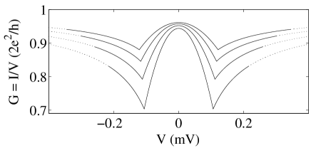
Figure 1: Conductance $G={I}/{V}$ as a function source-drain bias voltage, $V$, in the presence of single-electron and two-electron scattering. Solid lines mark the validity of the TLL model. Different traces are plotted at a fixed Fermi energy ($\epsilon_{F}\sim n^{2}\propto V_{g}^{2}$, where $V_{g}$ is the voltage on the QPC) ranging form $5K$ (lower curve) to $8K$ in steps of $1K$. We used GaAs parameters with $L=1\mu m$, $T=80mK$, and $\gamma\log\left({\lambda_{F}}/{d}\right)\approx 4.3$ (see text for definitions).

The kinks in Fig. 1 are due to the abrupt change in the parameter $K_{\rho}$, taken to be $K_{\rho}<1$ in the vicinity of the QPC, and $K_{\rho}=1$ at the broadening of the constriction. In an experimental realization, the transition between the two is smooth, and the kinks will be softened. A study of Eq. (Multiple Particle Scattering in Quantum Point Contacts) shows that for $T\ll eV$ and $K_{\rho}<1/4$, the contribution of the two electron scattering to the differential conductance may change sign. As a result the differential conductance at $eV>T_{L}$ may exceed the universal value $2e^{2}/h$, and the curvature at the high bias regime changes sign (not shown). From Eq. (7) it follows that at $\Theta\ll T_{L}$, the backscattering current is dominated by single-electron scattering, $\langle I_{\textrm{B}}(t)\rangle\approx\langle I_{\textrm{B}_{1}}(t)\rangle$. Conversely at $\Theta\lesssim T_{L}$, for an interacting system that exhibits an enhanced two-electron scattering, the current is given by $\langle I_{\textrm{B}}(t)\rangle\approx\langle I_{\textrm{B}_{2}}(t)\rangle$. At $T<eV$, the crossover voltage $V^{*}$ can be found by equating the two contributions to the backscattering current in Eq. (7), and is given by $eV^{*}=\sqrt{T_{L}^{2}G_{1}/G_{2}-\pi^{2}T^{2}}$.

Noise.-The occurrence of multi-particle scattering is accompanied by a distinctive signature on the shot noise of the system. Shot noise measures the size of charge-transfer events. As multi-particle scattering become frequent, the events that determine the shot noise consist of a charge which is larger than the single particle charge.

The expression for the symmetrized backscattering current correlator is found to be CommentNoise ; PonomarenkoPRB1999

$$\langle\delta I_{B}^{2}\rangle_{\omega=0} = \frac{2e\left\lvert\langle I_{\textrm{B}_{1}}\rangle\right\rvert}{\tanh\left({\beta eV}/{2\hbar}\right)}+\frac{4e\left\lvert\langle I_{\textrm{B}_{2}}\rangle\right\rvert}{\tanh\left(\beta eV/\hbar\right)}.$$ (11)

The noise behavior, depicted in Fig. 2, is affected by the competition between the single and two electron scattering events. At small $V\ll V^{*}$ corresponding to small backscattering current, two-electron scattering are scarce. Thus, the charge defined as the ratio $S/(2\left\lvert\langle I_{B}\rangle\right\rvert)$ is $e^{*}=e$. At $V>V^{*}$, corresponding to large backscattering current, two-electron scattering dominant the conductance, and the charge approaches $e^{*}\approx 2e$.

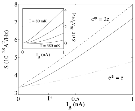
Figure 2: $S(\omega=0)=\langle\delta I_{T}^{2}\rangle_{\omega=0}$, as a function of $I_{B}$ (solid line), calculated using Ref. CommentNoise, , with $\langle\delta I_{B}^{2}\rangle_{\omega=0}$ given by Eq. (11), PonomarenkoPRB1999 at $eV<T_{L}$. Auxiliary plots represent the noise calculated with $\langle\delta I_{B}^{2}\rangle_{\omega=0}=\frac{2e^{*}\left\lvert I_{B}\right\rvert}{\tanh\left(\beta e^{*}V/2\hbar\right)}$, where $e^{*}=e$ (dotted line), and $e^{*}=2e$ (dashed line). $I^{*}$ is given by E. (7), with $V=V^{*}$. We have used the parameters of Fig. 1 with $\epsilon_{F}=7K$. Inset: Temperature dependence of the total noise, at $T$ from $80mK$ to $380mk$ in $100mK$ steps (thermal noise was subtracted).

While other existing models, e.g., the Kondo model, can account for increasing conductance at small SD bias MeirPRL2002 , the doubling of the charge is a unique feature of the model presented here. Moreover, the two models have different ranges of validity. The use of the Kondo model is justified at very low densities, where a single electron is believed to be localized at the point contact. Conversely the model presented here is valid at densities high enough to consider the TLL model. Thus, noise measurements performed at different ranges of parameters, can be used to distinguish the two behaviors.

Conclusion.- We have studied the spinfull TLL model with one- and two-electron scattering. Under proper conditions, the two electron scattering processes dominate the conductance of the system. We predict that at this limit, the shot noise will approach $e^{*}=2e$, and suggest noise measurements as a way to substantiate the validity of our model.

The interacting TLL with a single impurity scatterer, describes a large class of systems at the low energy limit. An example of which is the Hall bar contracted by means of a QPC. Within the TLL model, the backscattering of electrons at $\nu=1$, and of quasi particles at $\nu=\frac{1}{3}$ cannot account for the measured enhancement in the conductance at low bias voltage HeiblumCondMat2003 ; RoddaroCondMat2005 . Conversely, multiple particle backscattering prompt by the reduced density near the QPC, become scarce as the bias is lowered, leading to an enhanced conductance, concurring with the transport measurements. In a system dominated by $n$-particle scattering at high energies, we expect that the shot noise, at large backscattering current, will approach $e^{*}=n\nu e$. For example, at $\nu=1/3$, an enhanced three quasi-particle scattering, will result in an effective charge, that approaches $e^{*}=3\nu e=e$, at large backscattering current. The challenging task remains to find a microscopic model that predicts such an enhanced multiple particle scattering in the quantum Hall system.

Acknowledgements: We would like to thank A. M. Finkel’stein, Y. Gefen, L. Goren, B. I. Halperin, M. Heiblum, Y. Meir, N. Ofek, R. de Picciotto and A. Stern. The study was supported by Minerva and by an ISF grant 845/04.

References

- (1) T. Giamarchi, Quantum Physics in One Dimension, (Clarendon Press,Oxford, 2004).
- (2) D. C. Mattis, Phys. Rev. Lett. 32, 714 (1974).
- (3) K. A. Matveev, Dongxiao Yue, and L. I. Glazman, Phys. Rev. Lett. 71, 3351 (1993).
- (4) When short range interactions are considered, i.e., when the screening length is much smaller than the length of the QPC, the interacting length, , is determined by the latter. In the opposite limit, interactions are long-ranged, and is governed by the screening length. For simplicity we do not consider the crossover between the two. determines the range of energies over which the two scattering processes grow. Thus, When is longer, the scattering is enhanced, and the conductance is reduced.
- (5) O. M. Auslaender, A. Yacoby, R. de Picciotto, K. W. Baldwin, L. N. Pfeiffer, K. W. West, Science 295, 825 (2002).
- (6) A. M. Chang, Rev. Mod. Phys. 75, 1449 (2003).
- (7) N. K. Patel, J. T. Nicholls, L. Martin-Moreno, M. Pepper, J. E. F. Frost, D. A. Ritchie, and G. A. C. Jones, Phys. Rev. B 44, 13549 (1991); S. M. Cronenwett, H. J. Lynch, D. Goldhaber-Gordon, L. P. Kouwenhoven, C. M. Marcus, K. Hirose, N. S. Wingreen, and V. Umansky, Phys. Rev. Lett. 88, 226805 (2002).
- (8) S Roddaro, V Pellegrini, F Beltram, L. N. Pfeiffer, K. W. West, cond-mat/0501392, (2005).
- (9) Y. C. Chung, M. Heiblum, V. Umansky, Phys. Rev. Lett. 91, 216804 (2003).
- (10) Within our model , where , is the density in the 1D section, and is the gate voltage on the QPC. When the QPC is opened, increases and hence increases. In reality, the dependence on is much more complex. However it is clear that as increases, decreases due to efficient screening. These corrections will further increase as the QPC is opened.
- (11) K. A. Matveev Phys. Rev. Lett. 92, 106801 (2004).
- (12) In his paper MatveevPRL2004 , Matveev considers low densities where a WC is formed in the QPC, whereas the model described here is valid at higher densities, where the TLL model is applicable. Here , is the effective spin band width. We find that at these , two-electron scattering results in a power law resistance , as opposed to the WC model that predicts . Moreover we study the combined effect of an impurity scatterer and interactions. Conversely, the WC model assumes a smooth potential modulation with no impurities.
- (13) H. J. Schulz, Phys. Rev. Lett. 71, 1864 (1993).
- (14) Y. Oreg and A. M. Finkel’stein, Phys. Rev. Lett. 74, 3668 (1995); D. L. Maslov and M. Stone Phys. Rev. B 52, R5539 (1995).
- (15) A. Furusaki and N. Nagaosa Phys. Rev. B 47, 4631 (1993).
- (16) Interactions generate two-electron backscattering that can not be considered as two independent single electron processes. In diagramatic formulation, this amounts to all connected diagrams with four external legs (two incoming right movers and two outgoing left movers, and their hermitian conjugates). A first order calculation of these diagrams yields Eq. (5).
- (17) It should be noted that in the densities considered here, is not a small parameter. However, higher order terms are expected to further increase the scattering coefficient, as seen from the RG analysis.
- (18) G. D. Mahan, Many-Particle Physics 3rd. ed. (Plenum, New York, 2000); T. Martin cond-mat/0501208.
- (19) Dimensional counting shows that cross terms are of order of . These contradict the Fermi liquid theory (as they imply that the leading correction to the self energy is ). An explicit calculation shows that they vanish.
- (20) The relation between the zero frequency spectral density of the noise of the transmitted current, , and of the backscattering one, , is given by PonomarenkoPRB1999 .
- (21) V. V. Ponomarenko and N. Nagaosa, Phys. Rev. B 60, 16865 (1999).
- (22) Y. Meir, and A. Golub, Phys. Rev. Lett. 88, 116802 (2002); Y. Meir, K. Hirose, and N. S. Wingreen Phys. Rev. Lett. 89, 196802 (2002).