Current induced transverse spin-wave instability in thin ferromagnets: beyond linear stability analysis

Abstract

A sufficiently large unpolarized current can cause a spin-wave instability in thin nanomagnets with asymmetric contacts. The dynamics beyond the instability is understood in the perturbative regime of small spin-wave amplitudes, as well as by numerically solving a discretized model. In the absence of an applied magnetic field, our numerical simulations reveal a hierarchy of instabilities, leading to chaotic magnetization dynamics for the largest current densities we consider.

I Introduction

Almost a decade ago SlonczewskiSlonczewski (1996) and Berger Berger (1996) predicted that when a spin-polarized current is passed through a ferromagnet it transfers the transverse component of its spin angular momentum to the ferromagnet. The experimental verification of the theoretical predictions followed within a few years.Tsoi et al. (1998); Sun (1999); Wegrowe et al. (1999); Myers et al. (1999); Katine et al. (2000) Since then, the so-called ‘spin-transfer effect’ has been observed in a large number of different experiments.

In most experiments, the spin-transfer torque is studied in a ferromagnet–normal-metal–ferromagnet tri-layer structure where a thick ferromagnet first polarizes the current which then exerts a spin-transfer torque on a second thinner ferromagnet. At sufficiently large applied current densities, the spin-transfer torque then may alter the magnetization direction of the thin magnet. The observation of hysteretic magnetic switching for one current direction only was seen as a hallmark of the spin-torque effect,Myers et al. (1999) and excluded an explanation of the experiments in terms of the Faraday field associated with the applied current. (Note that for small system sizes, the spin-transfer torque, which scales proportional to the current density, dominates over the torque exerted by the magnetic field caused by the current flow,which is proportional to the total current.) Dynamical aspects of the magnetic switching process were addressed in recent experiments.Kiselev et al. (2003, 2004); Rippard et al. (2004); Krivorotov et al. (2004)

Over the past few years there has been much theoretical interest in understanding the spin-transfer torque and its consequences for hybrid ferromagnet–normal-metal devices. The connection between spin currents or spin accumulation in the normal metal spacer layer and the spin torque can be considered understoodWaintal et al. (2000); Stiles and Zangwill (2002); Xia et al. (2002) (see Ref. Tserkovnyak et al., 2004 for a recent review). Most calculations of the response of the magnetization to the spin-transfer torque have been done in the so-called ‘macrospin approximation’, assuming that the ferromagnets remain single domains during spin-transfer induced switching events.Sun (2000); Bazaliy et al. (2004); Li and Zhang (2004); Apalkov and Visscher (2004); Kovalev et al. (2005); Xiao et al. (2005) They have addressed the precise nature of the magnetic switching process, the possibility of limit cycles, and the temperature dependence of the spin-transfer torque. In addition, full micromagnetic simulations have been done by several groups,Li and Zhang (2003); Berkov and Gorn (2005a, b); Torres et al. (2005) e.g., to examine the effect of the Ampere field on the hysteretic switching or the breakdown of the macrospin model into quasi-chaotic dynamics at very high current densities. While the micromagnetic simulations are a significant improvement on the macrospin approximation when it comes accounting for spatial non-uniformities in the switching process, the existing simulations derive the spin-transfer torque from an externally fixed spin current, which is a poor description of the experimental geometries in which the spin currents are determined as an intricate combination of spin polarizations caused by all ferromagnetic elements in the device.Brataas et al. (2000); Waintal et al. (2000); Tserkovnyak et al. (2002, 2004)

In a recent work, two of the authors showed that a sufficiently large but unpolarized electrical current flowing perpendicular to a single thin ferromagnetic layer can excite spin waves in the ferromagnet.Polianski and Brouwer (2004) These spin waves have wavevector perpendicular to the direction of current flow. The key mechanism behind the transverse spin wave instability is electron diffusion in the normal-metal contacts perpendicular to the direction of current flow, see Fig. 1. Electrons backscattered from the ferromagnet are spin polarized, the polarization direction being antiparallel to the direction of the magnetization at the location where they were reflected from the ferromagnet. When these electrons reach the ferromagnetic layer a second time, they typically do so at a different point at the normal-metal–ferromagnet interface. In the presence of a spin wave, the magnetization direction of the ferromagnet will be different at that point, and these electrons will transfer the perpendicular component of their spin to the ferromagnet, thus exerting a spin-transfer torque. The sign of this torque is to enhance the spin-wave amplitude. A similar argument can be made for electrons transmitted through the ferromagnet, but their torques tend to suppress the spin-wave amplitude. Typically, source and drain contacts are asymmetric, and a net spin-transfer torque is exerted on the ferromagnet. This torque leads to a spin wave instability for the current direction in which the effect of backscattered electrons dominates, and not for the other current direction. Experiments on nanopillars a with single ferromagnetic layer have verified the theoretical predictions finding spin-wave instabilities for one direction of the current and for asymmetric junctions only.B. Özyilmaz, A. D. Kent, J. Z. Sun, M. J. Rooks, R. H. Koch (2004)

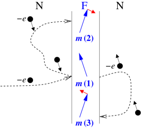
Figure 1: Through the spin-transfer torque, an unpolarized electrical current flowing perpendicular to a thin ferromagnetic layer can enhance or suppress spin waves. Electrons backscattered from the ferromagnet at point $1$ have their spin predominantly polarized antiparallel to magnetization direction $\mathbf{m}(1)$. These electrons exert a torque on the ferromagnet’s magnetization $\mathbf{m}(2)$ if they reach the ferromagnet a second time at point $2$, the direction of the torque being to enhance an existing spinwave [i.e., to increase any pre-existing difference between $\mathbf{m}(1)$ and $\mathbf{m}(2)$]. When electrons transmitted through the ferromagnet reach the ferromagnet a second time at point $3$, they exert a torque that suppresses an existing spinwave. If source and drain contacts are not symmetric, there is a net torque on the ferromagnet, which enhances or suppresses the spin wave, depending on current direction.

For a quantitative theory of this transverse spin-wave instability, an approach that combines a full self-consistent determination of the spin-transfer torque and, at the same time, goes beyond the macrospin approximation is essential.Polianski and Brouwer (2004) Indeed, the macrospin approximation does not allow for non-uniform spin waves in the ferromagnet, and, whereas an externally imposed spin transfer torque would predict a similar instability, a non-self-consistent theory would be quantitatively incorrect (e.g. predict the wrong wavelength for the spin wave) because it neglects the coupling between the spin current and the spin waves in the ferromagnet.

The possibility of current-induced non-uniform modes in heterostructures has become of recent interest in the field, both for single-layer and multilayer structures.Ji et al. (2003); Stiles et al. (2004); Urazhdin (2004); Brataas et al. (2005); Slavin and Kabos (2005); Özyilmaz et al. (2005) In particular, Ji, Chien, and StilesJi et al. (2003) reported experimental and theoretical evidence that for large ferromagnet thickness, ferromagnet–normal-metal junctions are unstable to the generation of non-uniform magnetization modes, but in this case, these are longitudinal modes (see also Refs. Myers et al., 1999 and Chen et al., 2004). Further, Stiles, Xiao, and Zangwill pointed out that transverse spinwaves can be excited even in symmetric junctions if the spinwave mode is at not uniform in the direction of current flow. However, excitation of these modes requires a higher currents than the transverse spin-waves considered here.Stiles et al. (2004)

Our previous work,Polianski and Brouwer (2004) as well as the other theoretical works on this and related spin-wave instabilities,Stiles et al. (2004); Brataas et al. (2005) was a linear stability analysis, sufficient to predict the onset of the instability, but not to describe the spin wave amplitude for current densities larger than the critical current density. Knowledge of the spin wave amplitude is necessary if one wants to study, e.g., how the spin wave instability affects the resistance of the normal-metal–ferromagnet junction. It is the goal of this present work to examine in detail the dynamics of the spin-wave beyond the instability. While we focus on the case of single-layers, we expect that, in light of the work of Refs. Brataas et al., 2005; Özyilmaz et al., 2005, our qualitative findings will carry over to the case of tri-layers and heterojunctions.

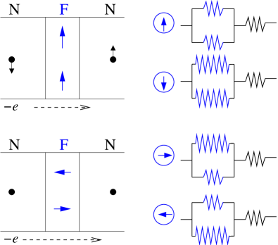
Figure 2: Spin will accumulate in normal metals on both sides of a ferromagnetic layer with uniform magnetization if an unpolarized current is passed through the ferromagnet (top left). A large-amplitude spinwave in the ferromagnet reduces the amount of spin polarization in the normal-metal regions adjacent to the ferromagnet and lowers the total resistance of the device (bottom left). This is shown schematically in the circuit diagrams (right). The top two circuit diagrams show the resistances seen by majority and minority electrons when the magnetization is spatially uniform, the short and long resistor symbols referring to minority and majority resistances, respectively. The ferromagnet with a large-amplitude spin wave can be seen as a parallel configuration of ferromagnets with opposite magnetization directions. The bottom two circuit diagrams show the resistances seen by two spin directions in this case. The net resistance is lower in the presence of a large-amplitude spin wave.

Although a quantitative description of how the spinwave instability affects the resistance of the normal-metal–ferromagnet junction will be postponed to the next two two sections, the sign of the effect can be determined using simple considerations. Once the current density has exceeded the critical current density for the spin wave excitation and a spin wave has been established, the fact that the magnetization is no longer uniform reduces the amount of spin accumulation in the normal metal contacts adjacent to the ferromagnet. A reduction of the spin accumulation in the normal metal contacts causes a reduction of the sample’s resistance, see Fig. 2 for a schematic drawing. Indeed, the experiments of Ref. B. Özyilmaz, A. D. Kent, J. Z. Sun, M. J. Rooks, R. H. Koch, 2004 observed a small decrease of the resistance of the nanopillar upon onset of the spin-wave instability. The effect of a purely transverse spinwave instability is opposite to that of a longitudinal spinwave, which increases the resistance of the device.Chen et al. (2004) The reduction of the spin accumulation in the normal-metal spacer also lowers the spin-transfer torque, thus providing a mechanism to saturate the growth of the spin wave amplitude for current densities larger than the critical current density. Moreover, note that a theory of this effect needs to combine features of both the micromagnetic approach and the self-consistent treatment of the spin-transfer torque.

In Sec. II we consider current densities slightly above the critical current density. In this regime, a perturbative treatment in the spin wave amplitude is possible. In Sec. III we then perform a detailed numerical simulation of a simplified system that allows us to probe current densities much larger than the critical current density. Whereas the observed magnetization dynamics in the presence of a large magnetic field is rather unsurprising — there is one stable energy minimum, and the magnetization precesses around the direction for which energy is minimal —, in the absence of an external magnetic field we find a hierarchy of instabilities. For very high currents the system shows chaotic behavior with measurable Lyapunov exponents.

II Perturbative calculation

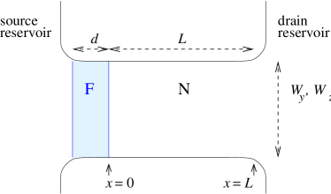
Figure 3: Schematic picture of the normal-metal–ferromagnet–normal-metal junction considered in our calculations. The ferromagnetic layer (F) is connected to source and drain reservoirs though normal metal spacers (N). We consider the maximally asymmetric case with only one spacer of length $L\gg l_{\rm sf}$.

We consider a single ferromagnetic layer, connected to source and drain reservoirs, see Fig. 3. Between the ferromagnet and the drain reservoir is a normal-metal spacer, as is common in nanopillar geometries. There is, however, no normal-metal spacer between the ferromagnet and the source reservoir. We use coordinates $x$, $y$, $z$, where $x$ is the coordinate perpendicular to the layer structure and $y$ and $z$ are coordinates in the plane of the layers.

Both the ferromagnet and the spacer layer have a rectangular cross section of dimensions $W_{y}\times W_{z}$. The ferromagnet has thickness $d$, which is taken small enough that the chemical potential for the conduction electrons and the the direction $\mathbf{m}$ of the magnetization of the ferromagnet do not depend on the longitudinal coordinate $x$. The normal metal spacer has thickness $L$. Transport through the normal metal spacer is diffusive, with conductivity $\sigma$.

In the normal metal spacer, the charge and spin degrees of the conduction electrons are described by the equations

$$\nabla^{2}\mu_{\rm c} = 0,\ \ \ j_{x}=(\sigma/e)\partial_{x}\mu_{\rm c},$$

$$l_{\rm sf}^{2}\nabla^{2}{\mbox{\boldmath$\mu$}}_{\rm s} = {\mbox{\boldmath$\mu$}}_{\rm s},\ \ \mathbf{j}_{\rm s}=-(\hbar\sigma/2e^{2})\partial_{x}{\mbox{\boldmath$\mu$}}_{\rm s},$$ (1)

where $\mu_{\rm c}$ and ${\mbox{\boldmath$\mu$}}_{\rm s}$ are chemical potentials for the electron density and electron spin respectively, $-e$ is the electron charge, and $l_{\rm sf}$ is the spin diffusion length in the normal metal spacer. Further, $j_{x}$ is the charge current density and $\sigma$ is the conductivity of the normal metal leads. The boundary conditions for $x=L$ at the drain reservoir is

$$\mu_{\rm c}(L)=-eV,\ \ \mbox{\boldmath$\mu$}_{\rm s}(L)=\mbox{{\boldmath$0$}}.$$ (2)

Here the argument $L$ refers to the $x$ coordinate. The $y$ and $z$ coordinates are not written explicitly. The second boundary is the interface between the normal-metal and ferromagnet at $x=0$. Since the electron dynamics happens on a time scale that is much faster than the rate of change of the magnetization direction $\mathbf{m}$, this boundary condition can be taken treating $\mathbf{m}$ in the adiabatic approximation,Brataas et al. (2000); Tserkovnyak et al. (2002)

$$j_{x}(0) = \frac{1}{e}\left[g_{+}\mu_{\rm c}(0)+g_{-}{\mathbf{m}}\cdot\mbox{\boldmath$\mu$}_{\rm s}(0)\right],$$

$$\mathbf{j}_{\rm s}(0) = -\frac{\hbar}{2e^{2}}\left(g_{-}\mu_{\rm c}(0)+g_{+}\mathbf{m}\cdot\mbox{\boldmath$\mu$}_{\rm s}(0)\right)\mathbf{m}$$ (3)

$$\mbox{}+\frac{\hbar}{2e^{2}}g_{1}\left(2\mbox{\boldmath$\mu$}_{\rm s}(0)\times\mathbf{m}+\hbar\dot{\mathbf{m}}\right)\times\mathbf{m}$$

$$\mbox{}+\frac{\hbar}{2e^{2}}g_{2}\left(2\mbox{\boldmath$\mu$}_{\rm s}(0)\times\mathbf{m}+\hbar\dot{\mathbf{m}}\right).$$

Here $g_{\pm}=(g_{\uparrow}\pm g_{\downarrow})/2$, where $g_{\uparrow}$ and $g_{\downarrow}$ are interface conductivities for spins aligned parallel and anti-parallel to ${\mathbf{m}}$, and $g_{1}+ig_{2}$ is the complex valued ‘mixing interface conductivity’. The argument “0” refers to a coordinate in the normal metal spacer, just outside the ferromagnetic layer. The charge current and the spin current parallel to $\mathbf{m}$ are continuous at the interface. In writing down Eq. (II) we assumed that the two ferromagnet–normal-metal interfaces are identical, so that the potentials $\mu_{\rm c}$ and $\mathbf{m}\cdot\mbox{\boldmath$\mu$}_{\rm s}$ drop equally over both interfaces of the ferromagnet; the component of $\mbox{\boldmath$\mu$}_{\rm s}$ perpendicular to $\mathbf{m}$ is zero in the ferromagnet. (It is the non-conservation of spin current perpendicular to $\mathbf{m}$ that gives rise to the spin transfer torque.) For Co/Cu and Fe/Cr interfaces, these conductivities are tabulated, see Refs. Stiles, 1996; Xia et al., 2002. Typical values are in the range $g_{2}\ll g_{1}\sim g_{\pm}\sim 10^{14}~{}\Omega^{-1}m^{-2}$. For any interface, one has the constraint $g_{1}>g_{+}>g_{-}$.Brataas et al. (2000)

We are interested in the situation in which the magnetization is allowed to vary in the direction perpendicular to the current flow. In this case a large enough current may cause spin-wave excitations perpendicular to the direction of current flow.Polianski and Brouwer (2004) To simplify the notation, we take the limit $L\gg l_{\rm sf}$. The spin and charge chemical potentials in the normal-metal spacer then have the general solution

$$\mu_{\rm c}(\mathbf{r}) = \sum_{\mathbf{q}}e^{iq_{y}y+iq_{z}z}a_{\rm c}(\mathbf{q})e^{-(q_{y}^{2}+q_{z}^{2})^{1/2}x}+\frac{eIx}{W_{y}W_{z}\sigma},$$

$$\mbox{\boldmath$\mu$}_{\rm s}(\mathbf{r}) = \sum_{\mathbf{q}}e^{iq_{y}y+iq_{z}z}e^{-(q_{y}^{2}+q_{z}^{2}+l_{\rm sf}^{-2})^{1/2}x}\mathbf{a}_{\rm s}(\mathbf{q}),$$ (4)

where $\mathbf{q}=(0,q_{y},q_{z})^{\rm T}$ is a wavevector in the $y$-$z$ plane. The components $q_{y}$ and $q_{z}$ take values $q_{y}=\pi n_{y}/W_{y}$, $q_{z}=\pi n_{z}/W_{z}$ with integers $n_{y}$ and $n_{z}$. The Fourier expansion coefficients $a_{\rm c}(\mathbf{q})$ and $\mathbf{a}_{\rm s}(\mathbf{q})$ are real and satisfy

$$a_{\rm c}(\mathbf{q})=a_{\rm c}(-\mathbf{q}),\ \ \mathbf{a}_{\rm s}(\mathbf{q})=\mathbf{a}_{\rm s}(-\mathbf{q}).$$ (5)

We further define the quantities

$$G_{\rm c}(\mathbf{q}) = (\sigma/2)(q_{y}^{2}+q_{z}^{2})^{1/2},$$ (6)

$$G_{\rm s}(\mathbf{q}) = (\sigma/2)(q_{y}^{2}+q_{z}^{2}+l_{\rm sf}^{-2})^{1/2},$$ (7)

which have the same dimension as the interface conductivities $g_{\pm}$, $g_{1}$, and $g_{2}$. With these definitions, the boundary condition (II) at the normal-metal–ferromagnet interface becomes

$$0 = -\frac{eI}{W_{y}W_{z}}+2\sum_{\mathbf{q}}e^{iq_{y}y+iq_{z}z}\left[G_{\rm c}(\mathbf{q})a_{\rm c}(\mathbf{q})+g_{\rm+}a_{\rm c}(\mathbf{q})+g_{\rm-}\mathbf{a}_{\rm s}(\mathbf{q})\cdot\mathbf{m}\right],$$

$$0 = \sum_{\mathbf{q}}e^{iq_{y}y+iq_{z}z}\left[2G_{\rm s}(\mathbf{q})\mathbf{a}_{\rm s}(\mathbf{q})+(g_{\rm-}a_{\rm c}(\mathbf{q})\mathbf{m}\right.\left.+g_{\rm+}\mathbf{a}_{\rm s}(\mathbf{q})\cdot\mathbf{m})\mathbf{m}-2g_{1}(\mathbf{a}_{\rm s}(\mathbf{q})\times\mathbf{m})\times\mathbf{m}-2g_{2}\mathbf{a}_{\rm s}(\mathbf{q})\times\mathbf{m})\right]$$ (8)

$$\mbox{}-\hbar g_{1}\dot{\mathbf{m}}\times\mathbf{m}-\hbar g_{2}\dot{\mathbf{m}}.$$

Although Eq. (II) gives a set of linear equations for the expansion coefficients $a_{\rm c}(\mathbf{q})$ and $\mathbf{a}_{\rm s}(\mathbf{q})$, a solution in closed form is not possible for arbitrary magnetization $\mathbf{m}(y,z)$. Instead, we expand around the uniform equilibrium direction. Hereto we introduce a second coordinate system with axes labeled $1$, $2$, and $3$, such that $\mathbf{m}$ points along the unit vector $\mathbf{e}_{3}$ in the absence of an applied current, and write

$$\mathbf{m}=m_{1}\mathbf{e}_{1}+m_{2}\mathbf{e}_{2}+(1-m_{1}^{2}-m_{2}^{2})^{1/2}\mathbf{e}_{3}.$$ (9)

We then perform a Fourier transform, similar to Eq. (II)

$$m_{j}(y,z)=\sum_{\mathbf{q}}m_{j}(\mathbf{q})e^{iq_{y}y+iq_{z}z},\ \ j=1,2,$$ (10)

where $m_{j}(\mathbf{q})=m_{j}(-\mathbf{q})$. Finally, expanding in powers of $m_{1}$ and $m_{2}$, we have solved the spin and charge chemical potentials to third order in $m_{1}$ and $m_{2}$, which parameterize the deviations from equilibrium.

In order to complete the calculation, we need to calculate the rate of change of the magnetization direction $\mathbf{m}$ in the presence of the current $I$. Hereto we use the Landau-Lifshitz-Gilbert equation,Lifschitz and Pitaevskii (1980); Gilbert (2004)

$$\dot{\mathbf{m}}=\alpha{\mathbf{m}}\times\dot{\mathbf{m}}+\mbox{\boldmath$\tau$}_{\rm ex}+\mbox{\boldmath$\tau$}_{\rm an}+\mbox{\boldmath$\tau$}_{\rm ne},$$ (11)

where $\alpha$ is the Gilbert damping coefficient, $\mbox{\boldmath$\tau$}_{\rm ex}$ is the torque arising from exchange, $\mbox{\boldmath$\tau$}_{\rm an}$ is the torque from the combined effect of magnetic anisotropy and an applied magnetic field, and $\mbox{\boldmath$\tau$}_{\rm ne}$ represents the current-induced spin-transfer torque. The latter readsYa. B. Bazaliy et al. (1998)

$$\mbox{\boldmath$\tau$}_{\rm ne} = \frac{\gamma}{Md}(\mathbf{j}_{\rm s}(0)-\mathbf{j}_{\rm s}(-d))\times\mathbf{m})\times\mathbf{m}$$ (12)

$$= -\frac{\hbar\gamma}{Mde^{2}}\left[g_{1}({\mbox{\boldmath$\mu$}}_{\rm s}\times{\bf m}+\hbar\dot{\mathbf{m}})\times{\bf m}\right.$$

$$\left.\mbox{}+g_{2}({\mbox{\boldmath$\mu$}}_{\rm s}\times{\bf m}+\hbar\dot{\mathbf{m}})\right].$$

Here the spin current $\mathbf{j}_{\rm s}(-d)$ is taken in the source reservoir, $M$ is the magnetization per unit volume and $\gamma$ is the gyromagnetic ratio. Note that the terms proportional to the time derivative $\dot{\mathbf{m}}$ have contributions from two interfaces while the contribution to the torque from the spin chemical potential has a contribution from the $x=0$ interface only. (All potentials are zero in the source reservoir.) The exchange torque $\mbox{\boldmath$\tau$}_{\rm ex}$ is

$$\mbox{\boldmath$\tau$}_{\rm ex}=J\gamma M\nabla^{2}\mathbf{m}\times\mathbf{m},$$ (13)

where $J$ is the exchange constant. To linear order in $m_{1}$ and $m_{2}$, the anisotropy torque $\mbox{\boldmath$\tau$}_{\rm an}$ can be written

$$\mbox{\boldmath$\tau$}_{\rm an} = -\frac{\gamma}{M}(k_{1}m_{1}\mathbf{e}_{1}+k_{2}m_{2}\mathbf{e}_{2})\times\mathbf{m},$$ (14)

where $k_{1}$ and $k_{2}$ describe the combined effect of magnetic anisotropy and an applied magnetic field. If anisotropy dominates over the effect of a magnetic field, higher-order terms in an expansion in powers of $m_{1}$ and $m_{2}$ will be highly sample specific. Although this case can be dealt with using the methods presented below, the result of the calculation has little predictive value if those coefficients are not known independently. Therefore, we focus on the opposite limit that the anisotropy term in Eq. (14) is dominated by magnetic field. Then higher-order terms in an expansion in powers of $m_{1}$ and $m_{2}$ are related to the first-order terms, and one has

$$\mbox{\boldmath$\tau$}_{\rm an}=(k\gamma/M)\mathbf{e}_{3}\times\mathbf{m}.$$ (15)

where we wrote $k_{1}=k_{2}=k$. For future reference, we combine the material constants $J$ and $2k=k_{1}+k_{2}$ into the combinations

$$q_{\rm f}^{2}=\frac{k}{JM^{2}},\mbox{\ \ }j_{\rm f}^{2}=\left(\frac{2e}{\hbar}\right)^{2}JM^{2}k,$$ (16)

which have the dimension of inverse length and current density, respectively.

We now proceed to report the result of our calculation. The lowest order result, indicated by a superscript “$(0)$”, is

$$a_{\rm c}^{(0)}(\mathbf{q}) = \frac{ej(g_{+}+2G_{\rm s}(0))}{g_{\rm m}(0)g_{-}}\delta_{\mathbf{q},0},$$

$$\mathbf{a}_{\rm s}^{(0)}(\mathbf{q}) = \frac{-ej}{g_{\rm m}(0)}\mathbf{e}_{3}\delta_{\mathbf{q},0}.$$ (17)

Here $j=I/W_{y}W_{z}$ is the current density andPolianski and Brouwer (2004)

$$g_{\rm m}(\mathbf{q})=\frac{(g_{+}+2G_{\rm s}(\mathbf{q}))(g_{+}+2G_{\rm c}(\mathbf{q}))}{g_{-}}-g_{-}.$$ (18)

Writing $\mu_{\rm c}(L)=-eV=-e(L/\sigma W_{y}W_{z}+R)I$, we conclude that the resistance $R$ of the ferromagnetic layer is

$$R=\frac{2}{W_{y}W_{z}}\frac{\sigma/l_{\rm sf}+g_{+}}{2g_{+}\sigma/l_{\rm sf}+g_{+}^{2}-g_{-}^{2}}.$$ (19)

For the zeroth-order solution, the spin potential $\mu_{\rm s}$ is collinear with $\mathbf{m}$ throughout the sample. Hence, to that order there is no current-induced torque. This is different when small deviations from the situation $\mathbf{m}=\mathbf{e}_{3}$ are taken into account to first order. One finds that the first-order corrections $a_{\rm c}^{(1)}(\mathbf{q})$ and $a_{\rm s3}^{(1)}(\mathbf{q})$ are zero. In order to represent the first-order contributions to the transverse spin potentials $a_{\rm s1}$ and $a_{\rm s2}$, we use spinor notation, $a_{\rm s}=(a_{\rm s1},a_{\rm s2})^{\rm T}$ and $m=(m_{1},m_{2})^{\rm T}$. Then, defining

$$D(\mathbf{q})=(g_{1}+G_{\rm s}(\mathbf{q}))^{2}+g_{2}^{2},$$ (20)

we find

$$a_{\rm s}^{(1)}(\mathbf{q}) = -\frac{ej}{g_{\rm m}(0)}m(\mathbf{q})+\frac{ej(G_{\rm s}(\mathbf{q})-G_{\rm s}(0))}{g_{\rm m}(0)D(\mathbf{q})}\left[(g_{1}+G_{\rm s}(\mathbf{q}))m(\mathbf{q})+ig_{2}\sigma_{2}m(\mathbf{q})\right]$$

$$\mbox{}+\frac{\hbar}{2D(\mathbf{q})}\left[g_{2}G_{\rm s}(\mathbf{q})\dot{m}(\mathbf{q})+(g_{1}^{2}+g_{1}G_{\rm s}(\mathbf{q})+g_{2}^{2})i\sigma_{2}\dot{m}(\mathbf{q})\right].$$

where $\sigma_{2}$ is the second Pauli matrix. Note that the first term on the right hand side is the response to a uniform rotation of the magnetization, while the second and third terms give the response to a non-uniform and time-dependent magnetization.

The potentials are substituted into Eq. (12) to find the current-induced torque, and then into the Landau-Lifshitz-Gilbert equation (11) to find the rate of change of the magnetization. The current-induced torque has contributions proportional to the time derivative $\dot{\mathbf{m}}$, which lead to a renormalization of the Gilbert damping parameter $\alpha$ and the the gyromagnetic ratio $\gamma$. The renormalized Gilbert damping parameter $\tilde{\alpha}$ and gyromagnetic ratio $\tilde{\gamma}=\gamma/\tilde{\beta}$ depend on the transverse wavevector $\mathbf{q}$ and read

$$\tilde{\alpha} = \alpha+\frac{\hbar^{2}\gamma(g_{1}+G_{\rm s}(\mathbf{q}))}{2Mde^{2}}\left[1-\frac{G_{\rm s}(\mathbf{q})^{2}}{D(\mathbf{q})}\right],$$

$$\tilde{\beta} = 1+\frac{\hbar^{2}\gamma g_{2}}{2Mde^{2}}\left[1+\frac{G_{\rm s}(\mathbf{q})^{2}}{D(\mathbf{q})}\right].$$ (22)

In the macrospin limit $q\rightarrow 0$, these modifications coincide with the renormalized values originally reported in Ref. Tserkovnyak et al., 2002.

Again using two-component spinor notation, the complete Landau-Lifshitz-Gilbert equation then becomes

$$(\tilde{\beta}\openone_{2}+i\sigma_{2}\tilde{\alpha})\dot{m}(\mathbf{q})=A(\mathbf{q})m(\mathbf{q}),$$ (23)

with

$$A(\mathbf{q}) = \tau_{\parallel}^{(1)}\openone_{2}-i\sigma_{2}\left[\tau_{\perp}^{(1)}+\frac{\hbar\gamma j_{\rm f}(q^{2}+q_{\rm f}^{2})}{2eq_{\rm f}M}\right]$$ (24)

$$\mbox{}+\sigma_{3}\frac{\gamma(k_{1}-k_{2})}{2M}$$

and

$$\tau_{\parallel}^{(1)}(\mathbf{q}) = \frac{\hbar\gamma ej}{Mde^{2}}\frac{g_{1}^{2}+g_{2}^{2}+g_{1}G_{\rm s}(\mathbf{q})}{g_{\rm m}(0)D(\mathbf{q})}[G_{\rm s}(\mathbf{q})-G_{\rm s}(0)],$$

$$\tau_{\perp}^{(1)}(\mathbf{q}) = \frac{\hbar\gamma ej}{Mde^{2}}\frac{g_{2}G_{\rm s}(\mathbf{q})}{g_{\rm m}(0)D(\mathbf{q})}[G_{\rm s}(\mathbf{q})-G_{\rm s}(0)].$$ (25)

In the absence of a current, any spatial modulation of the magnetization is damped. However, a sufficiently large positive current $I$ can overcome the damping, and cause a spatial modulation of $\mathbf{m}$ to grow in time, rather than decay. (A positive current $I$ corresponds to electron flow in the negative $x$ direction.) The instability condition is easily obtained from Eq. (23)

$$\tau_{\parallel}^{(1)}(\mathbf{q})\frac{\tilde{\beta}(\mathbf{q})}{\tilde{\alpha}(\mathbf{q})}>\frac{\hbar\gamma j_{\rm f}(q^{2}+q_{\rm f}^{2})}{2eq_{\rm f}M}+\tau_{\perp}^{(1)}(\mathbf{q}).$$ (26)

We can analyze this result in different limits. For a ferromagnetic layer with sufficiently small transverse dimensions, $W_{y},W_{z}\lesssim(l_{\rm sf}/q_{\rm f}^{2})^{1/3}$ if $l_{\rm sf}q_{\rm f}\gg 1$, the instability happens at wavevector $\mathbf{q}=(\pi/W_{y})\hat{y}$ or $\mathbf{q}=(\pi/W_{z})\hat{z}$, whichever is smallest, and the critical current follows directly from Eq. (26). For wider layers, the critical current density $j_{\rm c}$ and critical wavevector $\mathbf{q}_{\rm c}$ are found as the current-density wavevector pair for which the onset of the instability condition happens at the lowest current density.

This condition can be simplified in the limit of a very thin ferromagnetic layer, $d\to 0$, neglecting terms proportional to $g_{2}$ (which is numerically smaller than $g_{1}$), and for wavenumbers $q\ll q_{\rm f}$. We then find that the critical current follows from minimizing the relation

$$j_{\rm c}(\mathbf{q}) = \frac{\hbar^{2}\gamma g_{\rm m}(0)j_{\rm f}}{2Mq_{\rm f}e^{2}}\frac{q^{2}+q_{\rm f}^{2}}{1-(1+q^{2}l_{\rm sf}^{2})^{-1/2}}.$$ (27)

In the limit $l_{\rm sf}\gg 1/q_{\rm f}$, this givesPolianski and Brouwer (2004)

$$q_{\rm c}=(q_{\rm f}^{2}/2l_{\rm sf})^{1/3},\ \ j_{\rm c}=\frac{\hbar^{2}\gamma g_{\rm m}(0)q_{\rm f}j_{\rm f}}{2Me^{2}}.$$ (28)

(The result for $j_{\rm c}$ was reported incorrectly in Ref. Polianski and Brouwer, 2004. Note that the condition $q_{\rm c}\ll q_{\rm f}$, which was used to derive Eq. (27) is consistent with Eq. (28) if $l_{\rm sf}\gg 1/q_{\rm f}$.) Note that $q_{\rm f}$ increases with an applied magnetic field, so that this limit becomes relevant even for the case of a normal metal with strong spin relaxation if the magnetic field is large enough. In the limit $l_{\rm sf}\ll 1/q_{\rm f}$ of strong spin relaxation and weak anisotropy, one has

$$q_{\rm c}=(4/3)^{1/4}(q_{\rm f}/l_{\rm sf})^{1/2},\ \ j_{\rm c}=\frac{\hbar^{2}\gamma g_{\rm m}(0)j_{\rm f}}{Mq_{\rm f}l_{\rm sf}^{2}e^{2}}.$$ (29)

At the critical current density, the trajectory of the magnetization is a simple ellipse (circle in the case of large magnetic fields). The ellipse is described by the coordinate transformation $m_{1}=r(\cos\theta\cos\phi+\eta\sin\theta\sin\phi),$ and $m_{2}=r(\sin\theta\cos\phi-\eta\cos\theta\sin\phi).$ The solution of the magnetization dynamics at the critical current then gives $\phi=\omega_{0}t$ and $r$ constant, where $\omega_{0}^{2}=\omega_{+}^{2}-\omega_{-}^{2}$, $\eta=(\omega_{+}-\omega_{-})/\omega_{0}$ and

$$\omega_{+}^{-1} = \frac{2Mce^{2}q_{\rm f}\cos(2\theta)}{\gamma(q_{\rm f}^{2}+q_{\rm c}^{2})j_{\rm f}}$$ (30)

$$\mbox{}-\frac{2Mce^{2}q_{\rm f}g_{2}G_{\rm s}(\mathbf{q})\sin(2\theta)}{\gamma j_{\rm f}(q_{\rm f}^{2}+q_{\rm c}^{2})(g_{1}^{2}+g_{2}^{2}+g_{1}G_{\rm s}(\mathbf{q})))},$$

$$\omega_{-}^{-1} = \frac{2Mc\hbar}{\gamma(k_{1}-k_{2})}.$$ (31)

and $c,\theta$ are obtained from $\tilde{\alpha}=c\sin 2\theta,\tilde{\beta}=c\cos 2\theta$. For the case of a large applied magnetic field, $k_{1}=k_{2}=k$, and neglecting $g_{2}$, we have $\eta=1$ and

$$\omega_{0}=\hbar\gamma j_{\rm f}(q_{\rm c}^{2}+q_{\rm f}^{2})/(2eq_{\rm f}M).$$ (32)

Note that, although the applied current has a large effect on the stability of the ellipsoidal motion (precession is damped for $j<j_{\rm c}$ and unstable for $j>j_{\rm c}$), its effect on the precession frequency is small. To a good approximation, the precession frequency equals the ferromagnetic resonance frequency in the absence of a current.

Whereas the first-order calculation allows one to find the current density at which the spin-wave instability sets in and the angular form of the low-amplitude excitations, it does not provide information about the magnitude of the spinwave oscillation for $j>j_{\rm c}$, or about the effect of the spinwave oscillation on the resistance of the ferromagnetic layer. This information can only be obtained from the analysis of the magnetization dynamics beyond first-order in the amplitude. Such a program proceeds along the same lines as the first-order calculation shown above: Calculation of the potentials for charge and spin in the presence of a non-uniform and time-dependent magnetization, followed by a calculation of the current-induced torque and the rate of change of the magnetization. We have carried out this program to third order in $m_{1}$ and $m_{2}$, and list some of our general results in the appendix. However, as this calculation involves higher-order contributions to the anisotropy torque $\mbox{\boldmath$\tau$}_{\rm an}$, for which the expansion constants are unknown, we find that this calculation has little predictive value. Instead, we focus on the limit in which all magnetic anisotropy arises from an applied magnetic field. In this limit, $\mbox{\boldmath$\tau$}_{\rm an}$ is known, cf. Eq. (15), and a theoretical analysis is useful.

An important simplification is that the higher-order analysis is necessary for the Fourier components $m_{1}(\mathbf{q}_{\rm c})$ and $m_{2}(\mathbf{q}_{\rm c})$ at the critical wavevector only. Hence, we need to consider only a single Fourier component in our considerations below. Solving for the leading (second order) correction to the charge potential, we find an expression that depends on the magnetization amplitude, to second order in $m_{1}$ and $m_{2}$, and on the time derivatives. Only first-order time-derivatives appear, which can be eliminated using the Landau-Lifshitz-Gilbert equation (23). For the case of a large applied magnetic field, the magnetization precession is circular, and one has

$$m_{1}(\mathbf{q}_{\rm c})\dot{m}_{2}(\mathbf{q}_{\rm c})-m_{2}(\mathbf{q}_{\rm c})\dot{m}_{1}(\mathbf{q}_{\rm c})=\omega_{0}r(\mathbf{q}_{\rm c})^{2},$$ (33)

where we abbreviated

$$r(\mathbf{q}_{\rm c})^{2}=m_{1}(\mathbf{q}_{\rm c})^{2}+m_{2}(\mathbf{q}_{\rm c})^{2}.$$ (34)

The precession frequency $\omega_{0}$ given by Eq. (30) above. We then find

$$a_{\rm c}^{(2)}(0)=\frac{2(G_{\rm s}(0)-G_{\rm s}(\mathbf{q}_{\rm c}))r(\mathbf{q}_{\rm c})^{2}}{D(\mathbf{q}_{\rm c})g_{\rm m}(0)^{2}}$$

$$\mbox{}\times\left[\omega_{0}g_{\rm m}(0)\left(D(\mathbf{q}_{\rm c})-G_{\rm s}(\mathbf{q}_{\rm c})(g_{1}+G_{\rm s}(\mathbf{q}_{\rm c}))\right)\right.$$

$$\left.\mbox{}-2ej_{\rm c}\left(D(\mathbf{q}_{\rm c})+(G_{\rm s}(0)-G_{\rm s}(\mathbf{q}_{\rm c}))(g_{1}+G_{\rm s}(\mathbf{q}_{\rm c}))\right)\right]$$

Solving for the leading (third) order torque, we note that the third order torque depends not only on the magnetization amplitudes $m_{1}(\mathbf{q}_{\rm c})$ and $m_{2}(\mathbf{q}_{\rm c})$, but also on their time derivative $\dot{m}_{1}$ and $\dot{m}_{2}$. The time derivatives appear to first, second, and third order in the expansion. The dependence on $\dot{m}^{(3)}$ leads to the same modifications to the Gilbert damping and gyromagnetic ratio as for the first-order current-induced torque calculated above. The dependence on $\dot{m}^{(2)}$ is through the $3$-component only, which can be written as

$$\dot{m}_{3}^{(2)}=-m_{1}\dot{m}_{1}^{(1)}-m_{2}\dot{m}_{2}^{(1)}.$$ (36)

The first-order time derivatives $\dot{m}^{(1)}$ can be expressed in terms of $m_{1}$ and $m_{2}$ using Eq. (33) [or, in the general case, using Eq. (23)]. For the anisotropy torque $\tau_{\rm an}$ we take the contribution from the magnetic field only. Hence,

$$\tau_{\rm ex}(\mathbf{q}_{\rm c})+\tau_{\rm an}(\mathbf{q}_{\rm c}) = \frac{\hbar\gamma j_{\rm f}}{2eq_{\rm f}M}\left[q_{\rm c}^{2}+q_{\rm f}^{2}+\frac{q_{\rm c}^{2}}{2}r(\mathbf{q}_{\rm c})^{2}\right]$$ (37)

$$\mbox{}\times(-i\sigma_{2})m(\mathbf{q}_{\rm c}).$$

Thus proceeding, we find that the third-order equation for the rate of change of the magnetization direction reads

$$(\tilde{\beta}\openone_{2}+i\sigma_{2}\tilde{\alpha})\dot{m}(\mathbf{q})^{(3)}=A(\mathbf{q})^{(3)}m(\mathbf{q})^{(3)},$$ (38)

with

$$A(\mathbf{q}_{\rm c})^{(3)} = -\frac{1}{2}r(\mathbf{q}_{\rm c})^{2}\left[2\tau_{\parallel}^{(3)}(0)\openone_{2}-2i\sigma_{2}\tau_{\perp}^{(3)}(0)+\tau_{\parallel}^{(3)}(2\mathbf{q}_{\rm c})\openone_{2}-i\sigma_{2}\tau_{\perp}^{(3)}(2\mathbf{q}_{\rm c})+3\tilde{\alpha}\omega_{0}\openone_{2}+\frac{\hbar\gamma j_{\rm f}q_{\rm c}^{2}}{2eq_{\rm f}M}i\sigma_{2}\right],$$ (39)

and

$$\tau^{(3)}_{\parallel}(\mathbf{k}) = \frac{\hbar\gamma g_{1}}{Mde^{2}(g_{1}+G_{\mathbf{q}})}\left\{\frac{[g_{+}+2G_{\rm c}(\mathbf{k})][g_{+}+2G_{\rm s}(\mathbf{q})]-g_{-}^{2}}{[g_{+}+2G_{\rm c}(\mathbf{k})][g_{+}+2G_{\rm s}(\mathbf{k})]-g_{-}^{2}}\right\}$$ (40a)

$$\mbox{}\times\left\{\frac{ej}{g_{\rm m}(0)}[G_{\rm s}(\mathbf{k})-G_{\rm s}(0)]+\left[g_{1}\hbar\omega_{0}-\frac{2ej(g_{1}+G_{\rm s}(0))}{g_{\rm m}(0)}\right]\frac{G_{\rm s}(\mathbf{k})-G_{\rm s}(\mathbf{q})}{g_{1}+G_{\rm s}(\mathbf{q})}\right\},$$

$$\tau^{(3)}_{\perp}(\mathbf{k}) = \frac{\hbar\gamma g_{2}\,G_{\rm s}(\mathbf{q})[G_{\rm s}(\mathbf{k})-G_{\rm s}(\mathbf{q})]}{Mde^{2}[g_{1}+G_{\rm s}(\mathbf{q})]^{3}}\left\{\frac{[g_{+}+2G_{\rm c}(\mathbf{k})][g_{+}+2G_{\rm s}(\mathbf{q})]-g_{-}^{2}}{[g_{+}+2G_{\rm c}(\mathbf{k})][g_{+}+2G_{\rm s}(\mathbf{k})]-g_{-}^{2}}\left[g_{1}\hbar\omega_{0}-\frac{ej(g_{1}+G_{\rm s}(0))}{g_{\rm m}(0)}\right]\right.$$ (40b)

$$\left.\mbox{\hskip 108.405pt}+\frac{[(g_{+}-2g_{1})(2G_{\rm c}(\mathbf{k})+g_{+})-g_{-}^{2}][G_{\rm s}(\mathbf{q})-G_{\rm s}(0)]ej}{g_{\rm m}(0)[(g_{+}+2G_{\rm c}(\mathbf{k}))(g_{+}+2G_{\rm s}(\mathbf{k}))-g_{-}^{2}]}\right\}.$$

Solving the differential equation for $m$, one finds that the precession amplitude for current density $j$ slightly above the critical current density $j_{\rm c}$ reads

$$r(\mathbf{q}_{\rm c})^{2} = \frac{\hbar\gamma j_{\rm f}(j-j_{\rm c})}{eq_{\rm f}Mj_{\rm c}}\frac{\tilde{\alpha}(q_{\rm c}^{2}+q_{\rm f}^{2})}{\tilde{\beta}\left[2\tau^{(3)}_{\parallel}(0)+\tau^{(3)}_{\parallel}(2\mathbf{q}_{\rm c})-3\tau^{(1)}_{\parallel}(\mathbf{q}_{\rm c})\right]-\tilde{\alpha}\left[2\tau^{(3)}_{\perp}(0)+\tau^{(3)}_{\perp}(2\mathbf{q}_{\rm c})-\hbar\gamma j_{\rm f}q_{\rm c}^{2}/(2eq_{\rm f}M)\right]}.$$ (41)

The result takes a simpler form in the limit $g_{2}\to 0$ (since $g_{2}$ is numerically smaller than $g_{1}$), $d\to 0$, and $1/l_{\rm sf}\ll q_{\rm c}\ll q_{\rm f}$,

$$r(\mathbf{q}_{\rm c})^{2} = \frac{(j-j_{\rm c})(g_{+}^{2}-g_{-}^{2}+g_{+}\sigma/l_{\rm sf})}{j_{\rm c}(2g_{1}g_{+}+g_{+}\sigma/l_{\rm sf}-g_{+}^{2}+g_{-}^{2})}.$$ (42)

Since $g_{1}>g_{+}>g_{-}$ we conclude that the $r(\mathbf{q}_{\rm c})^{2}>0$ is positive if $j>j_{\rm c}$, which excludes hysteretic behavior.

In the same limit we can also calculate the change in frequency of the spinwave given by

$$\frac{\omega}{\omega_{0}}=1+\frac{q_{\rm c}^{2}r(\mathbf{q}_{\rm c})^{2}}{3(q_{\rm c}^{2}+q_{\rm f}^{2})}.$$ (43)

Since the prefactor of the second term is much smaller than unity, $q_{\rm c}\ll q_{\rm f}$ for the parameter regime of interest, we conclude that in the regime of perturbation theory, there is hardly any change from the ferromagnetic resonance frequency.

Finally, at the onset of the spin-wave instability, the resistance of the ferromagnetic layer acquires a small negative correction

$$\frac{R}{R_{0}} = 1+\frac{a_{\rm c}^{(2)}(0)}{a_{\rm c}^{(0)}(0)},$$ (44)

$$\approx 1-\frac{2(\sigma/l_{\rm sf}+3g_{1})g_{-}^{2}r(\mathbf{q}_{\rm c})^{2}}{(\sigma/l_{\rm sf}+g_{+})(g_{+}^{2}-g_{-}^{2}+g_{+}\sigma/l_{\rm sf})}.$$

(In the second line we took the limits $g_{2}\to 0$, $d\to 0$, and used $1/l_{\rm sf}\ll q_{\rm c}\ll q_{\rm f}$.) This resistance decrease is anticipated on physical grounds since the non-uniform mode allows for an increased transmission of minority elections that diffuse along the transverse direction — see Fig. 2 and the corresponding discussion in Sec. I.

III Numerical Calculation

The calculations in the preceding section are valid for currents close to the onset of the instability. For currents much larger than the critical current, we need to go beyond perturbation theory to obtain the dynamics. Hereto we numerically solve for the magnetization dynamics and its effect on the resistance of the ferromagnetic layer.

In our numerical analysis, we assume $W_{z}\ll W_{y}$ and impose that the magnetization direction $\mathbf{m}(y,z)$ does not depend on $z$. The remaining two-dimensional problem is replaced by a finite number of one-dimensional problems by substituting the normal-metal spacer and the ferromagnetic layer by $N$ normal metal channels, each attached to a magnet with magnetization direction $\mathbf{m}(n)$, $n=1,\ldots,N$. In order to model a higher-dimensional structure, electrons are allowed to diffuse between the channels, whereas the $N$ magnets interact via an exchange energy. A schematic drawing of this model is shown in Fig. 4.

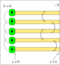
Figure 4: Schematic drawing of the model solved numerically. The continuous magnet is replaced by $N$ magnets (left), each coupled to a normal-metal wire (right). The wires are coupled via transverse diffusion (shown schematically as solid lines); the magnets are coupled via the exchange interaction (shown schematically as dashed lines).

In this discretized model, the potentials for charge and spin obey the equations

$$\partial^{2}_{x}\mu_{\rm c}(n,x) + \left(\frac{N}{W_{y}}\right)^{2}[\mu_{\rm c}(n+1,x)+\mu_{\rm c}(n-1,x)$$

$$\mbox{}-2\mu_{\rm c}(n,x)]=0,$$

$$\partial^{2}_{x}\mbox{\boldmath$\mu$}_{\rm s}(n,x) + \left(\frac{N}{W_{y}}\right)^{2}[\mbox{\boldmath$\mu$}_{\rm s}(n+1,x)+\mbox{\boldmath$\mu$}_{\rm s}(n-1,x)$$ (45)

$$\mbox{}-2\mbox{\boldmath$\mu$}_{\rm s}(n,x)]=\frac{\mbox{\boldmath$\mu$}_{\rm s}(n,x)}{l_{\rm sf}^{2}}.$$

Equations for the boundary channels, $n=1$ and $n=N$, are obtained by setting $\mu_{\rm c,s}(0,x)=\mu_{\rm c,s}(1,x)$ and $\mu_{\rm c,s}(N+1,x)=\mu_{\rm c,x}(N,x)$. The general solution of Eq. (45) is of the form

$$\mu_{\rm c}(n,x) = 2\sum_{l=0}^{N-1}a_{\rm c}(l)\cos\left[l\pi(n+1/2)/N\right]e^{-q_{\rm c}(l)x}$$

$$\mbox{}+\frac{eIx}{\sigma W_{y}W_{z}}.$$

$$\mbox{\boldmath$\mu$}_{\rm s}(n,x) = 2\sum_{l=0}^{N-1}\mathbf{a}_{\rm s}(l)\cos\left[l\pi(n+1/2)/N\right]e^{-q_{\rm s}(l)x},$$

with

$$q_{\rm c}(l)^{2} = 4(N/W_{y})^{2}\sin^{2}\left(l\pi/2N)\right),$$

$$q_{\rm s}(l)^{2} = l_{\rm sf}^{-2}+4(N/W_{y})^{2}\sin^{2}\left(l\pi/2N)\right).$$ (47)

The boundary conditions at $x=0$ (normal-metal–ferromagnet interface) are given by Eq. (II).

The magnetization dynamics is given by the Landau-Lifshitz-Gilbert equation (11), with a discretized exchange torque $\mbox{\boldmath$\tau$}_{\rm ex}$,

$$\mbox{\boldmath$\tau$}_{\rm ex}(n) = \frac{J\gamma MN^{2}}{W_{y}^{2}}\left[\mathbf{m}(n+1)+\mathbf{m}(n-1)\right]\times\mathbf{m}(n),$$

For the anisotropy torque we consider two different cases: The limit of a large applied magnetic field,

$$\mbox{\boldmath$\tau$}_{\rm an}=\frac{k\gamma}{M}\mathbf{e}_{3}\times\mathbf{m}(n),$$ (49)

as well as the case of no applied field, where we take a simple model for the torque arising from magnetocrystalline and shape anisotropy,

$$\mbox{\boldmath$\tau$}_{\rm an}(n) = -\frac{\gamma}{M}[k_{1}m_{1}(n)\mathbf{e}_{1}+k_{2}m_{2}(n)\mathbf{e}_{2}]\times\mathbf{m}(n).$$

The Landau-Lifshitz-Gilbert equation, together with the boundary conditions at $x=0$, are sufficient to determine the $4N$ expansion coefficients $a_{\rm c}(l)$ and $\mathbf{a}_{\rm s}(l)$, $l=0,\ldots,N-1$, and the time derivative of the magnetization directions $\mathbf{m}(n)$, $n=1,\ldots,N$. Our numerical procedure consists of first expressing $\dot{\mathbf{m}}(n)$ in terms of the potential expansion coefficients $a_{\rm c}(l)$ and $\mathbf{a}_{\rm s}(l)$ using the Landau-Lifshitz-Gilbert equation, and then solving for the potential expansion coefficients using the boundary condition at $x=0$.

For the practical implementation of this scheme, it is useful to define $3\times 3$ matrices ${\cal M}$ and ${\cal R}=\mathbf{m}\mathbf{m}^{T}$ such that for any vector ${\bf v}$, ${\bf v}\times\mathbf{m}={\cal M}{\bf v}$ and ${\cal R}-\openone_{3}={\cal M}^{2}$. In $3\times 3$ matrix notation, the time derivative of the magnetization vector can be expressed in terms of the potential coefficients as

$$\dot{\mathbf{m}}(n) = \frac{\beta^{\prime}\openone_{3}+\alpha^{\prime 2}{\cal R}/\beta^{\prime}-\alpha^{\prime}{\cal M}}{\alpha^{\prime 2}+\beta^{\prime 2}}$$ (51)

$$\mbox{}\times\left\{{\cal M}[\mbox{\boldmath$\tau$}_{\rm ex}+\mbox{\boldmath$\tau$}_{\rm an}]+\frac{2\hbar\gamma}{Mde^{2}}\sum_{l=0}^{N-1}[{\cal M}g_{1}+g_{2}\openone_{3}]{\cal M}\mathbf{a}_{\rm s}(l)\cos\left[l\pi(n+1/2)/N\right]\right\},$$

where $\alpha^{\prime}=\alpha+\hbar^{2}\gamma g_{1}/(Mde^{2})$ and $\beta^{\prime}=1+\hbar^{2}\gamma g_{2}/(Mde^{2})$. In turn, the potential coefficients $\mathbf{a}_{\rm s}(l)$ are obtained from inverting a $4N$ dimensional matrix equation,

$$\sum_{l=0}^{N-1}2\cos\left(l\pi(n+1/2)/N\right)\left[\begin{array}[]{cc}2\sigma q_{\rm c}(l)+2g_{+}&2\mathbf{m}^{\rm T}g_{-}\\ 2\mathbf{m}g_{-}&\sigma q_{\rm s}(l)\openone_{3}+4\chi_{1}\end{array}\right]\left(\begin{array}[]{c}a_{\rm c}(l)\\ {\mathbf{a}}_{\rm s}(l)\end{array}\right)=\frac{2eI}{W_{y}W_{z}}\left(\begin{array}[]{c}g_{+}\\ g_{-}\mathbf{m}\end{array}\right)+\left(\begin{array}[]{c}0\\ \mbox{\boldmath$\chi$}_{2}\end{array}\right),$$ (60)

where we abbreviated

$$\chi_{1}(n) = g_{-}{\cal R}-{\cal M}(g_{1}{\cal M}+g_{2}\openone_{3})$$ (61)

$$\mbox{}+\frac{\hbar^{2}\gamma}{2Mde^{2}(\alpha^{\prime 2}+\beta^{\prime 2})}(g_{1}{\cal M}+g_{2}\openone_{3})[\beta^{\prime}\openone_{3}+\alpha^{\prime 2}{\cal R}/\beta^{\prime}-\alpha^{\prime}{\cal M}]{\cal M}(g_{1}{\cal M}+g_{2}\openone_{3}),$$

$$\mbox{\boldmath$\chi$}_{2}(n) = \frac{2(g_{1}{\cal M}+g_{2}\openone_{3})\hbar^{2}\gamma}{Mde^{2}(\alpha^{\prime 2}+\beta^{\prime 2})}[\beta^{\prime}\openone_{3}+\alpha^{\prime 2}{\cal R}/\beta^{\prime}-\alpha^{\prime}{\cal M}]{\cal M}[\mbox{\boldmath$\tau$}_{\rm ex}(n)+\mbox{\boldmath$\tau$}_{\rm an}(n)].$$ (62)

We have performed numerical simulations for $N$ ranging between $10$ and $20$, although all data shown are for $N=10$ and $N=11$. We verified that there is no qualitative dependence on the parity of $N$ in our simulations. A small random torque was added at each time step to mimic the effect of a small but finite temperature. (The corresponding temperature obtained from the fluctuation-dissipation theorem was less then a mK.Apalkov and Visscher (2004))

Below we present our results. We first consider the case in which the anisotropy torque is dominated by an applied magnetic field, taking Eq. (49) for the anisotropy torque $\mbox{\boldmath$\tau$}_{\rm an}$. We then consider the case in which there is no applied magnetic field, taking Eq. (LABEL:eq:taueqnum2) for $\mbox{\boldmath$\tau$}_{\rm an}$. The latter case is qualitatively different from the former, as it has two stable equilibria for $\mathbf{m}$ ($\mathbf{m}=\mathbf{e}_{3}$ and $\mathbf{m}=-\mathbf{e}_{3}$), whereas in the presence of a large applied field the equilibrium position is at $\mathbf{m}=\mathbf{e}_{3}$.

III.1 Large applied magnetic field

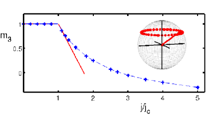
Figure 5: Main panel shows the magnetization component $m_{3}(1)$ of the first magnet, as a function of applied current. The solid line is obtained from the perturbation theory result (41), while the dashed line is a guide to the eye. In a large magnetic field, the motion is circular. an example is shown in the inset where $j=1.5j_{\rm c}$.

For the numerical simulations with a magnetic field, we took values for the various parameters as follows: thickness $d=0.2~{}\mathrm{nm}$, Width $W_{y}=55~{}\mathrm{nm}$, as is appropriate for typical nanopillar experiments,Katine et al. (2000) spin-diffusion length $l_{\rm sf}=100~{}\mathrm{nm}$, $\sigma/l_{\rm sf}=10^{15}\Omega^{-1}\mathrm{m}^{-2}$, $g_{1}=5.5\times 10^{14}~{}\Omega^{-1}\mathrm{m}^{-2}$, $g_{2}=0.3\times 10^{14}~{}\Omega^{-1}\mathrm{m}^{-2}$, $g_{\uparrow}=g_{+}+g_{-}=4.2\times 10^{14}~{}\Omega^{-1}\mathrm{m}^{-2}$, $g_{\downarrow}=g_{+}-g_{-}=3.3\times 10^{14}~{}\Omega^{-1}\mathrm{m}^{-2}$. The interface conductivities are taken from numerical calculations for a disordered Cu/Co interface;Xia et al. (2002) the conductivity $\sigma$ and the spin relaxation length $l_{\rm sf}$ are consistent with those in Cu. We further took $\alpha=0.01$, $\hbar\gamma g_{1}/Mde^{2}=0.0138$, $j_{\rm f}=10^{12}\mathrm{A}/\mathrm{m}^{2}$, $q_{\rm f}=10^{-1}\mathrm{nm}^{-1}$ (as is appropriate for Co, see Ref. Wohlfahrt, 1980; the magnetic field corresponding to the values of $j_{\rm f}$ and $q_{\rm f}$ listed above is of a strength comparable to the intrinsic anisotropy energy). For these parameters, the width of the sample is so small that the spinwave wavenumber $q$ is set by the finite sample width, $q=\pi/W_{y}$.

For current densities below $j_{\rm c}$, no spinwaves are excited. Simulation runs in which the magnetization is tilted away from the easy axis $\mathbf{e}_{3}$ show damped precession towards the equilibrium magnetization direction $\mathbf{m}=\mathbf{e}_{3}$. For current densities above $j_{\rm c}$, a spin-wave with wavenumber $q=\pi/W_{y}$ is excited. Each magnet $n$ in our simulation $n=1,\ldots,N$ shows circular precession around the direction of the applied magnetic field, see Fig. 5, inset. The amplitude of the oscillation increases with current as predicted by the perturbation theory of the preceding section. The $3$-component of the magnetization is a constant of the motion and can be monitored to measure the amplitude. Numerical results for $m_{3}$ for the magnet $n=1$ are shown in Fig. 5 as a function of current density, together with a comparison of our numerical results with the perturbative result (41). With a large applied field, the magnetization dynamics remains regular even for current densities much larger than $j_{\rm c}$. The effect of the spin-wave instability on the resistance of the ferromagnetic layer is shown in Fig. 6.

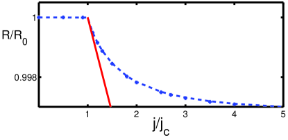
Figure 6: Resistance of the ferromagnetic layer, as a function of applied current (crosses). The solid line is obtained from the perturbation theory result (44), while the dashed line is a guide to the eye.

III.2 No applied magnetic field

We have also performed numerical simulations in the absence of an applied magnetic field. Hereto, we choose Eq. (LABEL:eq:taueqnum2) for the anisotropy torque, and choose $k_{1}$ and $k_{2}$ such that $(k_{1}-k_{2})/(k_{1}+k_{2})=0.99$. This form of the anisotropy is appropriate for thin magnetic layers, in which the magnetic anisotropy is predominantly of easy-plane type. The magnitude of the anisotropy energy is set by the parameters $q_{\rm f}$ and $j_{\rm f}$, for which we take the same values as in the previous subsection. All other parameters are also taken the same as in the previous subsection.

The magnetization dynamics without applied magnetic field is much richer than the magnetization dynamics at a large magnetic field. The reason is the existence of two stable equilibrium directions if no external magnetic field is applied ($\mathbf{m}=\mathbf{e}_{3}$ and $-\mathbf{e}_{3}$). At sufficiently large current densities, the current-induced torque drives the magnetization direction between these two stable directions, leading to a variety of dynamical phases.

For the numerical parameters chosen in our simulation, we observe the following characteristic dynamical modes: For current densities $j_{\rm c}<j\lesssim 2j_{\rm c}$ the instability develops with the wavenumber $q=\pi/W_{y}$. Because the magnetic anisotropy energy used for the simulation has no rotation symmetry around the $3$ axis, the magnetization direction $\mathbf{m}(n)$ of each magnet $n=1,\ldots,N$ traces out an ellipse, rather than a circle. We describe the magnetization motion is described using Poincaré sections for the polar angles $\theta$ and $\phi$ for the magnetization. The top right panel in Fig. 7 shows traces that are symmetric about $\phi=\pi$, which have the functional form for $\mathbf{m}$ as predicted by the perturbation theory in the preceding section.

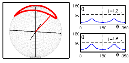
Figure 7: Typical elliptical trajectory for one of the discrete nanomagnets $\mathbf{m}(n)$ for weak easy axis and strong easy plane anisotropy with $j_{\rm c}<j<2j_{\rm c}$ (left panel). The upper and lower right panels show the corresponding Poincaré sections for $j=1.2j_{\rm c}$ and $1.5j_{\rm c}$ respectively. This regime agrees with the perturbative calculation of Sec. II, where the lowest energy spin-wave mode is excited and increasing the current only changes the amplitude of elliptical oscillation.

For higher currents with $2j_{\rm c}\lesssim j\lesssim 2.5j_{\rm c}$, the reflection symmetry about the easy axis is spontaneously broken, resulting in asymmetric ellipses (upper inset in Fig. 8), which for even higher current densities turn into orbits around the direction perpendicular to the easy axis (lower inset in Fig. 8). A three-dimensional rendering of this regime is shown in Figure 8.

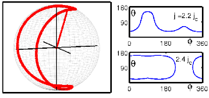
Figure 8: First manifestations of further dynamical instabilities in the range $2j_{\rm c}<j<2.5j_{\rm c}$. The upper right panel shows a Poincaré section for $j=2.2j_{\rm c}$ where the motion is no longer symmetric about the easy axis. The lower right panel shows the motion for $j=2.4j_{\rm c}$ where the motion is trapped between the $\pm\hat{e}_{3}$ easy axes direction. The left panel shows what this motion looks like on the unit sphere.

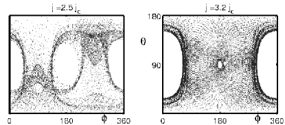
Figure 9: Poincaré sections for the magnetization direction of one of the magnets at $j=2.5j_{\rm c}$ (left) and $j=3.2j_{\rm c}$ (right).

For even larger currents there is a transition into non-periodic modes that cover a significant part of phase space, as shown in Figure 9. Whereas these modes are non-ergodic for lower current densities, they eventually become ergodic and chaotic at high current densities, with Lyapunov exponents increasing with the current density $j$ (data not shown).

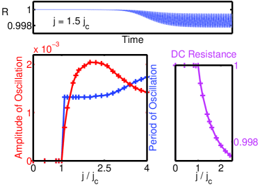
Figure 10: The upper panel shows the time trace of resistance where the spin-wave instability causes a decrease in the observed resistance. The lower left plot shows how the amplitude and period of the resistance oscillation change with the driving current, while the lower right panel shows the decrease of dc resistance.

In this general case, when the magnetization motion is not just simple circular precession, the spin-wave instability not only leads to a decrease of the dc resistance of the ferromagnetic layer, it also causes a fast oscillation of the resistance as shown in the time trace in Figure 10. The right panel in Fig. 10 shows the decrease of the dc resistance up to $j=2.5j_{\rm c}$. (No sufficiently accurate numerical results were obtained for larger current density.) Results for the variation of the resistance amplitude and frequency with the applied current density are shown in the left panel for current densities up to $4j_{\rm c}$. At the parameter values considered in our simulation, the onset of the non-periodic magnetization variations is accompanied by a sharp rise in precession frequency and a decrease of the amplitude of the resistance fluctuations.

IV Conclusion

We have presented a detailed study of the transverse spin-wave instability for a single ferromagnetic layer subject to a large current perpendicular to the layer. Our calculations have been in the small-amplitude regime, where perturbation theory can be used, and in the large-amplitude regime, where the magnetization dynamics can be solved numerically.

The two main signatures of the spin-wave instability are (1) existence of the instability for one current direction only, and (2) a small reduction in the dc resistance of the ferromagnetic layer. The resistance decrease arises because the existence of a spin wave with large amplitude lowers the spin accumulation in the normal metal adjacent to the ferromagnet. A lower spin accumulation corresponds to a lower resistance (just as a high spin accumulation state of the antiparallel configuration in the standard current-perpendicular-to-plane giant magnetoresistance geometry gives a high resistance state). Both features have been seen in a recent experiment.B. Özyilmaz, A. D. Kent, J. Z. Sun, M. J. Rooks, R. H. Koch (2004)

An important question for a dynamical instability is whether or not it is hysteretic. Our calculation has shown that the instability studied here is not, if a large magnetic field is applied. Without applied magnetic field, the nature of the spin wave instability depends on the precise form of the magnetic anisotropy, and both hysteretic and non-hysteretic behavior can be expected, in principle.

A noteworthy aspect of our calculation is that the spin-transfer torque is calculated self-consistently: the magnitude and direction of the spin-transfer torque depends on the spin accumulation in the normal metal, which, in turn, depends on the precise magnetization profile of the ferromagnet. In doing this, our work connects the the circuit theory for hybrid ferromagnet–normal-metal systems, which has been used extensively to describe the magnet’s effect on spin accumulations in macrospin approximation,Tserkovnyak et al. (2004) and micromagnetic simulations, which, to date, have been restricted to simplified models for the spin-transfer torque. However, our simulations should be considered a proof-of-principle. They lack the spatial resolution and sophistication that full-scale micromagnetic simulations have.

Appendix

The perturbative calculation of Sec. II focused on the case of a large applied magnetic field because, in that case, theoretical results for the spin wave amplitude do not depend on sample-dependent anisotropy energies. In this appendix we outline the theory for the general case.

For the most general case, one needs a better ansatz for the intrinsic torque $\mbox{\boldmath$\tau$}_{\rm an}$ than Eqs. (14) or (15), as well as an expression for the current-induced torque that does not rely on rotation symmetry around the easy axis. The general expression for the torque $\mbox{\boldmath$\tau$}_{\rm an}$ is most conveniently derived from the Free energy, $\mbox{\boldmath$\tau$}_{\rm an}=-(\gamma/M)(\partial F/\partial\mathbf{m})\times\mathbf{m}$. Since we are interested in the mode $\mathbf{m}(\mathbf{q}_{\rm c})$ only, we can expand $F$ in powers of $m_{1}(\mathbf{q}_{\rm c})$ and $m_{2}(\mathbf{q}_{\rm c})$, up to fourth oder as

$$F(\mathbf{m}) = \frac{1}{2}\left[k_{1}m_{1}(\mathbf{q}_{\rm c})^{2}+k_{2}m_{2}(\mathbf{q}_{\rm c})^{2}\right]$$ (63)

$$\mbox{}+\sum_{j=0}^{3}k_{j}^{\prime}m_{1}(\mathbf{q}_{\rm c})^{j}m_{2}(\mathbf{q}_{\rm c})^{3-j}$$

$$\mbox{}+\sum_{j=0}^{4}k_{j}^{\prime\prime}m_{1}(\mathbf{q}_{\rm c})^{j}m_{2}(\mathbf{q}_{\rm c})^{4-j}.$$

The higher-order expansion constants $k_{j}^{\prime}$, $j=0,1,2,3$, and $k_{j}^{\prime\prime}$, $j=0,1,\ldots,4$, are not governed by any special symmetry and therefore likely to be sample specific. (The cubic terms in the expansion of $F(\mathbf{m})$ may be forbidden if there is a reflection symmetry around the easy axis. However, there is no such symmetry in the presence of an applied magnetic field that is not aligned with the one of the sample’s easy or hard axes, so that cubic terms need to be included in a general treatment.) Note that the higher-order torque terms are as important in determining the spin wave amplitude as the higher-order current-induced spin-transfer torque. Unless these coefficients are known independently, a calculation of the spin wave amplitude has no predictive value — that was the reason why the main text addressed the case of a large applied magnetic field.

We now list our general results for the second and third order potentials and third-order spin-transfer torque. The symbols used are defined in Sec. II of the main text. The second-order charge potential expansion coefficients for the normal-metal spacer are

$$a_{\rm c}^{(2)}(\mathbf{q}) = ej\sum_{\mathbf{q}^{\scriptstyle{\prime}}}\left\{\frac{[G_{\rm s}(0)+G_{\rm s}(\mathbf{q})-2G_{\rm s}({\mathbf{q}{\scriptscriptstyle{{}^{\prime}}}})]D({\mathbf{q}^{\scriptstyle{\prime}}})+2[G_{\rm s}(0)-G_{\rm s}({\mathbf{q}{\scriptscriptstyle{{}^{\prime}}}})][G_{\rm s}(\mathbf{q})-G_{\rm s}({\mathbf{q}{\scriptscriptstyle{{}^{\prime}}}})][g_{1}+G_{\rm s}({\mathbf{q}{\scriptscriptstyle{{}^{\prime}}}})]}{D({\mathbf{q}^{\scriptstyle{\prime}}})g_{\rm m}(0)g_{\rm m}(\mathbf{q})}\right.$$ (64)

$$\ \ \ \ \mbox{}\times[m_{1}({\mathbf{q}^{\scriptstyle{\prime}}})m_{1}(\mathbf{q}-{\mathbf{q}^{\scriptstyle{\prime}}})+m_{2}({\mathbf{q}^{\scriptstyle{\prime}}})m_{2}(\mathbf{q}-{\mathbf{q}^{\scriptstyle{\prime}}})]$$

$$\ \left.\mbox{}-\frac{2g_{2}[G_{\rm s}(0)-G_{\rm s}(\mathbf{q})][G_{\rm s}(\mathbf{q})-G_{\rm s}({\mathbf{q}{\scriptscriptstyle{{}^{\prime}}}})]}{D(\mathbf{q}^{\prime})g_{\rm m}(0)g_{\rm m}(\mathbf{q})}[m_{1}({\mathbf{q}^{\scriptstyle{\prime}}})m_{2}(\mathbf{q}-{\mathbf{q}^{\scriptstyle{\prime}}})-m_{2}({\mathbf{q}^{\scriptstyle{\prime}}})m_{1}(\mathbf{q}-{\mathbf{q}^{\scriptstyle{\prime}}})]\right\}$$

$$-\hbar\sum_{{\mathbf{q}^{\scriptstyle{\prime}}}}\left\{\frac{g_{2}[G_{\rm s}(\mathbf{q})-G_{\rm s}({\mathbf{q}{\scriptscriptstyle{{}^{\prime}}}})]G_{\rm s}(\mathbf{q})}{D({\mathbf{q}^{\scriptstyle{\prime}}})g_{\rm m}(\mathbf{q})}[m_{1}(\mathbf{q}-{\mathbf{q}^{\scriptstyle{\prime}}})\dot{m}_{1}({\mathbf{q}^{\scriptstyle{\prime}}})+m_{2}(\mathbf{q}-{\mathbf{q}^{\scriptstyle{\prime}}})\dot{m}_{2}({\mathbf{q}^{\scriptstyle{\prime}}})]\right.$$

$$\ \left.\mbox{}+\frac{[G_{\rm s}(\mathbf{q})-G_{\rm s}({\mathbf{q}{\scriptscriptstyle{{}^{\prime}}}})][D({\mathbf{q}^{\scriptstyle{\prime}}})-G_{\rm s}({\mathbf{q}{\scriptscriptstyle{{}^{\prime}}}})(g_{1}+G_{\rm s}({\mathbf{q}{\scriptscriptstyle{{}^{\prime}}}}))]}{D({\mathbf{q}^{\scriptstyle{\prime}}})g_{\rm m}(\mathbf{q})}[m_{1}(\mathbf{q}-{\mathbf{q}^{\scriptstyle{\prime}}})\dot{m}_{2}({\mathbf{q}^{\scriptstyle{\prime}}})-m_{2}(\mathbf{q}-{\mathbf{q}^{\scriptstyle{\prime}}})\dot{m}_{1}({\mathbf{q}^{\scriptstyle{\prime}}})]\right\}.$$

The coefficient $a_{\rm c}^{(2)}(0)$ determines how the spin wave instability affects the resistance of the ferromagnetic layer, cf. Eq. (44) in the main text. The second order correction to the $3$-component of the spin potential is given by the expansion coefficients

$$\mathbf{a}_{\rm s3}^{(2)}(\mathbf{q}) = ej\sum_{\mathbf{q}^{\scriptstyle{\prime}}}\left\{\frac{1}{2g_{\rm m}(0)}[m_{1}({\mathbf{q}^{\scriptstyle{\prime}}})m_{1}(\mathbf{q}-{\mathbf{q}^{\scriptstyle{\prime}}})+m_{2}({\mathbf{q}^{\scriptstyle{\prime}}})m_{2}(\mathbf{q}-{\mathbf{q}^{\scriptstyle{\prime}}})]\right.$$ (65)

$$\ \left.\mbox{}-\frac{1}{D({\mathbf{q}^{\scriptstyle{\prime}}})g_{\rm m}(0)g_{\rm m}(\mathbf{q})}\left[D({\mathbf{q}^{\scriptstyle{\prime}}})(g_{+}+2G_{\rm c}(\mathbf{q}))(G_{\rm s}(0)+G_{\rm s}(\mathbf{q})-2G_{\rm s}({\mathbf{q}{\scriptscriptstyle{{}^{\prime}}}}))\right.\right.$$

$$\ \ \ \ \ \ \left.\left.\mbox{}-(G_{\rm s}(0)-G_{\rm s}({\mathbf{q}{\scriptscriptstyle{{}^{\prime}}}}))(g_{1}+G_{\rm s}(\mathbf{q}))(g_{\rm m}(\mathbf{q})-2(g_{+}+2G_{\rm c}(\mathbf{q})))(G_{\rm s}(\mathbf{q})-G_{\rm s}({\mathbf{q}{\scriptscriptstyle{{}^{\prime}}}}))\right]\right.$$

$$\ \ \ \ \mbox{}\times[m_{1}({\mathbf{q}^{\scriptstyle{\prime}}})m_{1}(\mathbf{q}-{\mathbf{q}^{\scriptstyle{\prime}}})+m_{2}({\mathbf{q}^{\scriptstyle{\prime}}})m_{2}(\mathbf{q}-{\mathbf{q}^{\scriptstyle{\prime}}})]$$

$$\ \left.\mbox{}-\frac{g_{2}[G_{\rm s}(0)-G_{\rm s}(\mathbf{q})][2(g_{+}+2G_{\rm c}(\mathbf{q}))(G_{\rm s}(\mathbf{q})-G_{\rm s}({\mathbf{q}{\scriptscriptstyle{{}^{\prime}}}}))-g_{\rm m}(\mathbf{q})]}{D({\mathbf{q}^{\scriptstyle{\prime}}})g_{\rm m}(0)g_{\rm m}(\mathbf{q})}[m_{1}(\mathbf{q})m_{2}(\mathbf{q}-{\mathbf{q}^{\scriptstyle{\prime}}})-m_{2}(\mathbf{q})m_{1}(\mathbf{q}-{\mathbf{q}^{\scriptstyle{\prime}}})]\right\}$$

$$\mbox{}-\hbar\sum_{{\mathbf{q}^{\scriptstyle{\prime}}}}\left\{\frac{g_{2}G_{\rm s}({\mathbf{q}{\scriptscriptstyle{{}^{\prime}}}})[g_{\rm m}(\mathbf{q})-2(g_{+}+2G_{\rm c}(\mathbf{q}))(G_{\rm s}(\mathbf{q})-G_{\rm s}({\mathbf{q}{\scriptscriptstyle{{}^{\prime}}}}))]}{2D({\mathbf{q}^{\scriptstyle{\prime}}})g_{\rm m}(\mathbf{q})}[m_{1}(\mathbf{q}-{\mathbf{q}^{\scriptstyle{\prime}}})\dot{m}_{1}({\mathbf{q}^{\scriptstyle{\prime}}})+m_{2}(\mathbf{q}-{\mathbf{q}^{\scriptstyle{\prime}}})\dot{m}_{2}({\mathbf{q}^{\scriptstyle{\prime}}})]\right.$$

$$\ \mbox{}-\frac{[D({\mathbf{q}^{\scriptstyle{\prime}}})-G_{\rm s}({\mathbf{q}{\scriptscriptstyle{{}^{\prime}}}})(g_{1}+G_{\rm s}({\mathbf{q}{\scriptscriptstyle{{}^{\prime}}}}))][g_{\rm m}(\mathbf{q})-2(g_{+}+2G_{\rm c}(\mathbf{q}))(G_{\rm s}(\mathbf{q})-G_{\rm s}({\mathbf{q}{\scriptscriptstyle{{}^{\prime}}}}))]}{2D({\mathbf{q}^{\scriptstyle{\prime}}})g_{\rm m}(\mathbf{q})}$$

$$\left.\ \ \ \ \mbox{}[m_{1}(\mathbf{q}-{\mathbf{q}^{\scriptstyle{\prime}}})\dot{m}_{2}({\mathbf{q}^{\scriptstyle{\prime}}})-m_{2}(\mathbf{q}-{\mathbf{q}^{\scriptstyle{\prime}}})\dot{m}_{1}({\mathbf{q}^{\scriptstyle{\prime}}})]\vphantom{\frac{M}{M}}\right\},$$

The very first term describes the effect of a uniform magnetization rotation; the remaining terms are the result of a non-uniform magnetization. There are second-order corrections to the spin potential expansion coefficients $a_{1}$ and $a_{2}$ that arise from the presence of cubic terms in the anisotropy Free energy. Such cubic terms cause second-order contributions to the time derivatives $\dot{m}_{1}$ and $\dot{m}_{2}$, which give a contribution to the second order spin potentials $a^{(2)}$ in the same way as the first-order time contribution to the time derivative affects the first-order spin potentials $a^{(1)}$, see Eq. (LABEL:eq:afirst).

Instead of listing the third-order potentials $a^{(3)}$, we describe the corresponding current-induced torque. We specialize to the contributions that are cubic in the magnetization amplitude at wavevector $\mathbf{q}_{\rm c}$. The resulting torque has terms proportional to the third-order contributions to the time derivatives of the magnetization. These terms give rise to a renormalized Gilbert damping coefficient and a renormalized gyromagnetic ratio, see Eq. (22). The remaining terms can be written as $2\tilde{}\mbox{\boldmath$\tau$}(0)+\tilde{}\mbox{\boldmath$\tau$}(2\mathbf{q}_{\rm c})$, where (again using two-component spinor notation)

$$\tilde{\tau}^{(3)}(\mathbf{k}) = \frac{-\hbar\gamma}{2Mde^{2}D(\mathbf{q}_{\rm c})^{2}g_{\rm m}(0)g_{\rm m}(\mathbf{k})}$$

$$\mbox{}\times\left\{2ejg_{2}D(\mathbf{q}_{\rm c})G_{\rm s}(\mathbf{q}_{\rm c})[G_{\rm s}(\mathbf{q}_{\rm c})-G_{\rm s}(\mathbf{k})][g_{+}+2G_{\rm c}(\mathbf{k})][G_{\rm s}(0)-G_{\rm s}(\mathbf{q}_{\rm c})]i\sigma_{2}m(\mathbf{q}_{\rm c})m^{\rm T}(\mathbf{q}_{\rm c})m(\mathbf{q}_{\rm c})\right.$$

$$\ \mbox{}-[g_{\rm m}(\mathbf{k})+2(g_{+}+2G_{\rm c}(\mathbf{k}))(G_{\rm s}(\mathbf{q}_{\rm c})-G_{\rm s}(\mathbf{k}))]$$

$$\mbox{}\times\big{[}-ej[(2G_{\rm s}(\mathbf{q}_{\rm c})-G_{\rm s}(0)-G_{\rm s}(\mathbf{k}))D(\mathbf{q}_{\rm c})+2(G_{\rm s}(0)-G_{\rm s}(\mathbf{q}_{\rm c}))(g_{1}+G_{\rm s}(\mathbf{q}_{\rm c}))(G_{\rm s}(\mathbf{q}_{\rm c})-G_{\rm s}(\mathbf{k}))]$$

$$\ \ \ \ \mbox{}\times[D(\mathbf{q}_{\rm c})-G_{\rm s}(\mathbf{q}_{\rm c})(g_{1}+G_{\rm s}(\mathbf{q}_{\rm c}))]m(\mathbf{q}_{\rm c})m^{\rm T}(\mathbf{q}_{\rm c})m(\mathbf{q}_{\rm c})$$

$$\ \mbox{}+ejg_{2}G_{\rm s}(\mathbf{q}_{\rm c})[G_{\rm s}(\mathbf{q}_{\rm c})-G_{\rm s}(\mathbf{k})][D(\mathbf{q}_{\rm c})+2(G_{\rm s}(0)-G_{\rm s}(\mathbf{q}_{\rm c}))(g_{1}+G_{\rm s}(\mathbf{q}_{\rm c}))]i\sigma_{2}m(\mathbf{q}_{\rm c})m^{\rm T}(\mathbf{q}_{\rm c})m(\mathbf{q}_{\rm c})$$

$$\ \mbox{}+\hbar g_{2}G_{\rm s}(\mathbf{q}_{\rm c})g_{\rm m}(0)[G_{\rm s}(\mathbf{q}_{\rm c})-G_{\rm s}(\mathbf{k})][D(\mathbf{q}_{\rm c})-G_{\rm s}(\mathbf{q}_{\rm c})(g_{1}+G_{\rm s}(\mathbf{q}_{\rm c}))]\dot{m}(\mathbf{q}_{\rm c})m^{\rm T}(\mathbf{q}_{\rm c})m(\mathbf{q}_{\rm c})$$

$$\ \mbox{}+(\hbar/2)[G_{\rm s}(\mathbf{q}_{\rm c})-G_{\rm s}(\mathbf{k})]D(\mathbf{q}_{\rm c})g_{\rm m}(0)[D(\mathbf{q}_{\rm c})-G_{\rm s}(\mathbf{q}_{\rm c})(2g_{1}+G_{\rm s}(\mathbf{q}_{\rm c}))]$$

$$\ \ \ \ \mbox{}\times[m(\mathbf{q}_{\rm c})m^{\rm T}(\mathbf{q}_{\rm c})i\sigma_{2}\dot{m}(\mathbf{q}_{\rm c})-i\sigma_{2}m(\mathbf{q}_{\rm c})m^{\rm T}(\mathbf{q}_{\rm c})\dot{m}(\mathbf{q}_{\rm c})]$$

$$\ \mbox{}+(\hbar/2)[G_{\rm s}(\mathbf{q}_{\rm c})-G_{\rm s}(\mathbf{k})]g_{\rm m}(0)[(D(\mathbf{q}_{\rm c})-G_{\rm s}(\mathbf{q}_{\rm c})(g_{1}+G_{\rm s}(\mathbf{q}_{\rm c})))^{2}-(g_{2}G_{\rm s}(\mathbf{q}_{\rm c}))^{2}]i\sigma_{2}\dot{m}(\mathbf{q}_{\rm c})m^{\rm T}(\mathbf{q}_{\rm c})m(\mathbf{q}_{\rm c})\left.\big{]}\right\}.$$

Once the perturbative expansions for the anisotropy torque and the current-induced spin-transfer torque are known, the Landau-Lifshitz-Gilbert equation can be solved for the magnetization dynamics.

References

- Slonczewski (1996) J. C. Slonczewski, J. Magn. Magn. Mater. 159, 1 (1996).
- Berger (1996) L. Berger, Phys. Rev. B 54, 9353 (1996).
- Tsoi et al. (1998) M. Tsoi, A. G. M. Jansen, J. Bass, W.-C. Chiang, M. Seck, V. Tsoi, and P. Wyder, Phys. Rev. Lett. 80, 4281 (1998).
- Sun (1999) J. Z. Sun, J. Magn. Magn. Mater. 202, 157 (1999).
- Wegrowe et al. (1999) J.-E. Wegrowe, D. Kelly, Y. Jaccard, P. Guittienne, and J.-P. Ansermet, Europhys. Lett. 45, 626 (1999).
- Myers et al. (1999) E. Myers, D. Ralph, J. Katine, R. Louie, and R. Buhrman, Science 285, 867 (1999).
- Katine et al. (2000) J. A. Katine, F. J. Albert, R. A. Buhrman, E. B. Myers, and D. C. Ralph, Phys. Rev. Lett. 84, 3149 (2000).
- Kiselev et al. (2003) S. I. Kiselev, J. C. Sankey, I. N. Krivorotov, N. C. Emley, R. J. Schoelkopf, and R. A. Buhrman, Nature 425, 380 (2003).
- Kiselev et al. (2004) S. I. Kiselev, J. C. Sankey, I. N. Krivorotov, N. C. Emley, M. Rinkoski, C. Perez, R. A. Buhrman, and D. C. Ralph, Phys. Rev. Lett. 93, 036601 (2004).
- Rippard et al. (2004) W. H. Rippard, M. R. Pufall, S. Kaka, S. E. Russek, and T. J. Silva, Phys. Rev. Lett. 92, 027201 (2004).
- Krivorotov et al. (2004) I. N. Krivorotov, N. C. Emley, A. G. F. Garcia, J. C. Sankey, S. I. Kiselev, D. C. Ralph, and R. A. Buhrman, Phys. Rev. Lett. 93, 166603 (2004).
- Waintal et al. (2000) X. Waintal, E. Myers, P. Brouwer, and D. Ralph, Phys. Rev. B 62, 12317 (2000).
- Stiles and Zangwill (2002) M. D. Stiles and A. Zangwill, Phys. Rev. B 66, 014407 (2002).
- Xia et al. (2002) K. Xia, P. J. Kelly, G. E. W. Bauer, A. Brataas, and I. Turek, Phys. Rev. B 65, 220401 (2002).
- Tserkovnyak et al. (2004) Y. Tserkovnyak, A. Brataas, G. E. W. Bauer, and B. I. Halperin, cond-mat/0409242 (2004).
- Sun (2000) J. Z. Sun, Phys. Rev. B 62, 570 (2000).
- Bazaliy et al. (2004) Y. B. Bazaliy, B. A. Jones, and S.-C. Zhang, Phys. Rev. B 69, 094421 (2004).
- Li and Zhang (2004) Z. Li and S. Zhang, Phys. Rev. B 69, 134416 (2004).
- Xiao et al. (2005) J. Xiao, A. Zangwill, and M. D. Stiles, cond-mat/0504142 (2005).
- Apalkov and Visscher (2004) D. Apalkov and P. Visscher, cond-mat/0405305 (2004).
- Kovalev et al. (2005) A. Kovalev, G. Bauer, and A. Brataas, cond-mat/0504705 (2005).
- Li and Zhang (2003) Z. Li and S. Zhang, Phys. Rev. B 68, 024404 (2003).
- Berkov and Gorn (2005a) D. Berkov and N. Gorn, Phys. Rev. B 71, 052403 (2005a).
- Torres et al. (2005) L. Torres, L. Lopez-Diaz, E. Martinez, M. Carpentieri, and G. Finocchio, J. Magn. Mag. Mater. 286, 381 (2005).
- Berkov and Gorn (2005b) D. Berkov and N. Gorn, cond-mat/0503754 (2005b).
- Brataas et al. (2000) A. Brataas, Y. V. Nazarov, and G. E. W. Bauer, Phys. Rev. Lett. 84, 2481 (2000).
- Tserkovnyak et al. (2002) Y. Tserkovnyak, A. Brataas, and G. E. W. Bauer, Phys. Rev. Lett. 88, 117601 (2002).
- Polianski and Brouwer (2004) M. L. Polianski and P. W. Brouwer, Phys. Rev. Lett. 92, 026602 (2004).
- B. Özyilmaz, A. D. Kent, J. Z. Sun, M. J. Rooks, R. H. Koch (2004) B. Özyilmaz, A. D. Kent, J. Z. Sun, M. J. Rooks, R. H. Koch, Phys. Rev Lett. 93, 176604 (2004).
- Ji et al. (2003) Y. Ji, C. L. Chien, and M. D. Stiles, Phys. Rev. Lett. 90, 106601 (2003).
- Stiles et al. (2004) M. D. Stiles, J. Xiao, and A. Zangwill, Phys. Rev. B. 69, 054408 (2004).
- Özyilmaz et al. (2005) B. Özyilmaz, A. D. Kent, M. J. Rooks, and J. Z. Sun, Phys. Rev. B 71, 140403 (2005).
- Urazhdin (2004) S. Urazhdin, Phys. Rev. B. 69, 134430 (2004).
- Brataas et al. (2005) A. Brataas, Y. Tserkovnyak, and G. Bauer, cond-mat/0501672 (2005).
- Slavin and Kabos (2005) A. Slavin and P. Kabos, IEEE Trans. Mag. 41, 1264 (2005).
- Chen et al. (2004) T. Y. Chen, Y. Ji, C. L. Chien, and M. D. Stiles, Phys. Rev. Lett. 93, 026601 (2004).
- Stiles (1996) M. D. Stiles, J. Appl. Phys. 79, 5805 (1996).
- Lifschitz and Pitaevskii (1980) E. M. Lifschitz and L. P. Pitaevskii, Statistical Physics, part 2 (Pergamon, 1980).
- Gilbert (2004) T. L. Gilbert, IEEE Trans. Mag. 40, 3443 (2004).
- Ya. B. Bazaliy et al. (1998) Ya. B. Bazaliy, B. A. Jones, and S.-C. Zhang, Phys. Rev. B 57, 3213 (1998).
- Wohlfahrt (1980) E. P. Wohlfahrt, in Ferromagnetic Materials, edited by E. P. Wohlfahrt (North-Holland, 1980), vol. 1.