Ferroelectricity Induced by Incommensurate Magnetism

Abstract

Ferroelectricity has been found to occur in several insulating systems, such as TbMnO₃ (TMO) and Ni₃V₂O₈ (NVO) which have more than one phase with incommensurately modulated long-range magnetic order. Here we give a phenomenological model which relates the symmetries of the magnetic structure as obtained from neutron diffraction to the development and orientation of a spontaneous ferroelectric moment induced by the magnetic ordering. This model leads directly to the formulation of a microscopic spin-phonon interaction which gives explains the observed phenomena. The results are given in terms of gradients of the exchange tensor with respect to generalized displacements for the specific example of NVO. It is assumed that these gradients will now be the target of first-principles calculations using the LDA or related schemes.

I Introduction

Recently studies have focussed on a a family of multiferroics which display a phase transition in which there simultaneously develops long-range incommensurate magnetic and uniform ferroelectric order. The most detailed studies have been carried out on the system Ni₃V₂O₈ (NVO).Rogado ; LawesKenzelmann ; FERRO ; EXPT A similar analysis of TbMnO₃ (TMO) has also appeared.TMO1 ; TMO2 (For a review of both systems see, see Ref. REV, .) To illustrate the phenomenon we show in Fig. 1 data for the spontaneous polarization as a function of applied magnetic field.

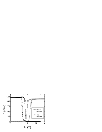
Figure 1: Adapted from Ref. FERRO, . Spontaneous polarization of NVO versus magnetic field applied along the $a$ and $c$ axes.

This data indicates a strong coupling between the magnetic order parameters and the polarization order parameters. To interpret the effect of this coupling, we reproduce in Fig.

Figure 2: Adapted from Ref. LawesKenzelmann, . Phase diagram of NVO for magnetic fields up to 8 T applied along the a direction (top) and along the c direction (bottom). P (AF) denotes the paramagnetic (antiferromagnetic) phase. For $H||{\bf c}$ there is no phase boundary between the P and AF phases. The arrowed vertical lines indicate the paths followed in Fig. 1.

2 the phase diagram as function of temperature $T$ and magnetic field $H$ applied along the crystal a and c-axes. Here we show the three magnetic phases that occur for $T\geq 2$K. The HTI and LTI phases are two distinct incommensurate phases. A spontaneous polarization appears throughout the LTI phase, but does not appear in the other phases. Thus, applying a strong enough $H$ to cross the LTI-AF phase boundary will kill the spontaneous polarization for ${\bf H}||{\bf c}$ or allow it for ${\bf H}||{\bf a}$. Since this transition is discontinuous, the hysteresis shown in Fig. 1 is to be expected.

This phenomenon has been explainedFERRO on the basis of a phenomenological model which invokes a Landau expansion in terms of the order parameters describing the incommensurate magnetic order and the order parameter describing the uniform spontaneous polarization. Already from this treatment it was clear that a microscopic model would have to involve a trilinear interaction Hamiltonian proportional to the product of two spin variables and one displacement variable. Furthermore, the symmetry requirements of the phenomenological model would naturally be realized by a proper microscopic model. In this paper we summarize the symmetry analysis and briefly describe the microscopic formulation which underlies the symmetry analysis.

II Symmetry of the Magnetic Phases

We first discuss the crystal structure of NVO. The space group of NVO is Cmca (#62 in

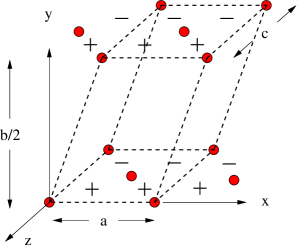
Figure 3: Positions in NVO of Ni cross-tie sites (filled circles) and Ni spine sites (indicated by $+$ and $-$ signs according to whether their $y$ coordinate is larger than or less than that of the layer). The dashed lines outline the primitive unit cell.

Ref. HAHN, ). Apart from the primitive translations ${\bf a}_{1}=(a/2)\hat{i}+(b/2)\hat{j}$, ${\bf a}_{2}=(a/2)\hat{i}-(b/2)\hat{j}$, and ${\bf a}_{3}=c\hat{k}$), the generators of the space group may be taken to be $2_{x}$ a two-fold rotation about the $x$-axis, $m_{x}$, a reflection taking $x$ into $-x$, and $m_{z}$ a glide plane which takes $z$ into $-z$, followed by a translation of $(b/2)\hat{j}+(c/2)\hat{k}$. The primitive unit cell contains two formula units of NVO and the magnetism is due to the Ni ions (see Fig. 3). There are two crystallographically inequivalent Ni sites which we will refer to as ”spine” and ”cross-tie” sites. The positions of the spine sites within the unit cell are ${\bf r}_{1}=(a/4,d,c/4)$, ${\bf r}_{2}=(a/4,-d,3c/4)$, ${\bf r}_{3}=(3a/4,-d,3c/4)$, and ${\bf r}_{4}=(3a/4,d,c/4)$. The parameter $d\approx 0.13b$ indicates that the a-c planes are buckled kagomé-like planes. The cross-tie sites within the unit cell are at ${\bf r}_{5}=(0,0,0)$ and ${\bf r}_{6}=(a/2,0,c/2)$.

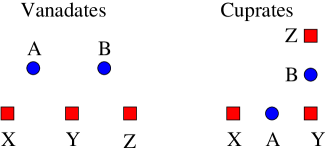
Figure 4: First and second neighbor exchanges paths (respectively X-A-Y or Y-B-Z and X-A-B-Z) in the vanadatesRogado (left) and cuprates (right), where A and B are oxygen ions and X, Y, and Z are magnetic ions. In the vandates the first neighbor exchange path is nearly a 90^o path, so that the nn exchange is weak, whereas in the cuprates the path is a $180$ path, so that here $J_{2}/J_{1}\sim 0.1$ (see Ref. 2342, ), whereas for the vanadates $J_{2}/J_{1}$ is much larger.EXPT

The Ni spins form weakly coupled chains (or spines) parallel to the ${\bf a}$-axis. The nearest neighbor (nn) and next-nearest neighbor (nnn) antiferromagnetic interactions ($J_{1}$ and $J_{2}$, respectively) along the spine compete with one another because, as shown in Fig. 4, in contrast to the situation in the cuprates, in the vanadates the nn interaction is anomalously weak. A result of this competition is that the spins order in an incommensurate state whose wavevector, $q$, along the ${\bf a}$ axis is given byNagamiya

$$\cos(aq/2)=-J_{1}/(4J_{2})\ .$$ (1)

As the temperature is lowered (at zero magnetic field), the system first orders in the HTI phase. Here the spins develop order mainly along the easy (a) axis so that their magnitude varies sinusoidally. At a lower temperature the LTI phase is entered in which there is additional ordering of the transverse spin components to more nearly satisfy the constraint of fixed spin length.

Figure 5: Two adjacent $x-z$ planes in NVO (buckling not shown). Complex spin amplitudes for wavevector $q$ (whose real part gives the spin moment). Here $2_{x}$ is the axis of two-fold rotation about $x$ and $m_{z}$ represents the glide plane which consists of the mirror plane shown at $z=c/4$ together with the displacement $b/2$ along $y$ (from one plane to the next).

The above description of the incommensurate phases is too simplistic. Accordingly we now turn to a more detailed discussion which takes proper account of the structure within each unit cell. The $\alpha$-component of the spin order at position ${\bf R}$ (which is the $\tau$th site in the unit cell) is expressed in terms of Fourier components at wavevector $q$ as

$$S_{\alpha\tau}({\bf R}) = [S_{\alpha\tau}({\bf q})e^{i{\bf q}\cdot{\bf R}}+S_{\alpha\tau}({\bf q})^{*}e^{-i{\bf q}\cdot{\bf R}}]/2\ ,$$ (2)

where $S_{\alpha\tau}({\bf q})$ is a complex-valued Fourier coefficient and $S_{\alpha\tau}(-{\bf q})=S_{\alpha\tau}({\bf q})^{*}$. In Fig. 5 we show the complex quantity $S_{\alpha\tau}({\bf q})e^{i{\bf q}\cdot{\bf R}}$ whose real part gives the spin order at position ${\bf R}$. Assuming only a single Fourier wavevector condenses (see below), we see that the spin structure is characterized by the six vector Fourier components of the unit cell. Since these quantities are three component vectors and each components is complex-valued, this structure is characterized by 36 real-valued parameters. As we shall see, the use of symmetry drastically reduces the number of parameters needed to characeterize the magnetic structure.

Translational invariance indicates that the Landau expansion of the free energy at quadratic order in terms of these Fourier components must assume the form

$$F_{2} = \sum_{\bf q}F_{2}({\bf q})\ ,$$ (3)

where

$$F_{2}({\bf q}) = \sum_{\alpha\alpha^{\prime};\tau\tau^{\prime}}c_{\alpha\tau;\alpha^{\prime}\tau^{\prime};{\bf q}}S_{\alpha\tau}(-{\bf q})S_{\alpha^{\prime}\tau^{\prime}}({\bf q})\ .$$ (4)

The eigenvalues of the quadratic form $F_{2}({\bf q})$ are the various inverse susceptibilities. We are interested in the stability of the quadratic form (since we assume the ordering transition is a continuous one). We may plot the least positive (least stable) eigenvalue as a function of wavevector $q$.

Figure 6: Inverse susceptibility as a function of wavevector for a sequence of temperatures for the $J_{1}$, $J_{2}$ model with $J_{1}/J_{2}=2.56$ (as for NVO). Temperature is in units of $J_{1}$.

Such plots for a sequence of temperatures are shown in Fig. 6, where one sees that some value of wavevector is selected at which the paramagnetic phase first becomes unstable relative to the formation of long-range order. Of course, this value of $q$ is determined by the interactions between spins, which are not well known. Here we are interested in what can be said on the basis of symmetry. A cardinal principle is that we always reject the possibility of accidental degeneracy. That is, there is only a single value of $q$ which becomes unstable as the temperature is lowered from the paramagnetic phase. (This phenomenon is called wavevector selection.) For a ferromagnet, the selected wavevector is $q=0$ and for a simple cubic antiferromagnetic $q=(\pi/a)(1,1,1)$, where $a$ is the lattice constant. For NVO the situation is more complicated because along each spine one has competing nn and nnn antiferromagnetic interactions which cause the inverse susceptibility to have its minimum at some nonspecial value of wavevector. This value isLawesKenzelmann ${\bf q}\approx 0.28(2\pi/a)\hat{i}$. The unit cell contain several spins, so that the actual incommensurate spin configuration can realize different symmetries within the unit cell. In the HTI phase one has incommensurate spin ordering mainly on the spines in which the spins are oriented along the easy (${\bf a}$) axis with sinusoidally varying amplitude. In the LTI phase, in addition to the order preexisting in the HTI phase, significant spin order transverse to the ${\bf a}$ axis appears, mainly on the cross-tie sites. Superficially, this type of structure may seem difficult to characterize. However, by focussing on the symmetry of the structure we are able to obtain a convincing phenomenological analysis of the symmetry of the magnetoelectric interaction.

We therefore now turn to the an analysis of the magnetic symmetry. Since the wavevector lies along the $x$-axis, the free energy, $F_{2}({\bf q})$ must be invariant under the operations of the crystal which leave the $x$-axis invariant. The group of these symmetry operations includes the identity operation ${\cal E}$, a two fold rotation about the $x$-axis, $2_{x}$, the glide reflection through a $z$-plane, $m_{z}$ and $2_{x}m_{z}$. (Some of these are illustrated in Fig. 5.) Without going through the details of group theory, one can say (in this case) that the eigenvector of the quadratic form $F_{2}({\bf q})$, must also be an eigenvector of the operation $2_{x}$ (with eigenvalue either $+1$ or $-1$) and also of $m_{z}$ (with eigenvalue either $+1$ and $-1$). Thus the structure determination is much simplified. Instead of having to determine the 6 complex vectors ${\bf S}_{n}$ of Fig. 5, we use the fact that these spin components form a vector which is simultaneously an eigenvector of $F_{2}({\bf q})$, $2_{x}$, and $m_{z}$. Accordingly we may specify (or guess) the four possible sets of eigenvalues of $2_{x}$ and $m_{z}$. This set of eigenvalues is technically known as the irreducible representation $\Gamma$, or irrep, for short. The actual active irrep is selected as the one which best fits the diffraction data. For the HTI phase the active irrep is found to beLawesKenzelmann $\Gamma_{4}$ for which the eigenvalues of $2_{x}$ and $m_{z}$ are $-$ and $+$, respectively. For this irrep we have to specify the 3 complex spin amplitudes of a single spine site and the $y$ and $z$ components of a single cross-tie site. The other amplitudes are then determined by application of the symmetry operators $2_{x}$ and $m_{z}$. Since we reject accidental degeneracy, the ordering of the HTI phase can only involve a single irrep. In Fig.

Figure 7: As Fig. 5. Fourier coefficients $S_{\alpha\tau}(q)$ in terms of symmetry-adapted parameters for the HTI irrep $\Gamma=\Gamma_{4}$, for which the eigenvalues of $2_{x}$ and $m_{z}$ are $-1$ and $+1$, respectively.

7, we show the spin function for the HTI phase of NVO corresponding to the eigenvalues of $2_{x}$ and $m_{z}$ respectively $-1$ and $+1$.LawesKenzelmann Notice that the characterization of the magnetic structure is reduced to the specification of only five complex-valued symmetry adapted coordinates.

When the LTI phase is entered, the situation is much the same. In addition to a spin function with the HTI symmetry, we now introduce additional ordering which has a different symmetry. This additional symmetry is found to correspond to the eigenvalues of $2_{x}$ and $m_{z}$ respectively $+1$ and $+1$ (of irrep $\Gamma_{1}$) and the corresponding spin functions (which require the specification of four additional symmetry adapted coordinates) are shown in Fig. 8.

Figure 8: As Fig. 5. Fourier coefficients $S_{\alpha\tau}(q)$ in terms of symmetry-adapted parameters for the LTI irrep $\Gamma=\Gamma_{1}$, for which the eigenvalues of $2_{x}$ and $m_{z}$ are both $+1$.

The cystal NVO is inversion symmetric and we have not yet discussed how this affects the analysis. Under spatial inversion ${\cal I}$ the components of spin transform into each other. Since spin is a pseudovector, inversion does not change the orientation of the spin, but takes it into the spatially inverted position and therefore takes $q$ into $-q$ (which is the same as complex conjugation). Also inversion takes the site ${\bf r}_{1}$ in the unit cell into site ${\bf r}_{3}$ and site ${\bf r}_{2}$ into site ${\bf r}_{4}$. Referring to Figs. 7 and 8, one see that we have defined the spin components $m_{s\alpha}^{(n)}$ with appropriate phase factors of $i$ so thatFOOT

$${\cal I}m_{s\alpha}^{(n)} = {m_{s\alpha}^{(n)}}^{*}\ .$$ (5)

This same relation also holds for the cross-tie order parameters without the necessity of introducing phase factors. Now consider the expansion of the free energy in terms of these variables, where for notational convenience we set (for each irreducible representation) $\xi_{1}(q)=m_{sx}(q)$, $\xi_{2}(q)=m_{sy}(q)$, $\xi_{3}(q)=m_{sy}(q)$, and $\xi_{4}(q)$, and if need be, $\xi_{5}(q)$ are similar cross-tie order parameters. In terms of these variables the quadratic free energy is

$$F_{2}({\bf q}) = \sum_{n,n^{\prime};\Gamma}c_{n,n^{\prime}}^{\Gamma}\xi_{n}^{\Gamma}(q)^{*}\xi_{n^{\prime}}^{\Gamma}(q)\ ,$$ (6)

where the superscript identifies the irreducible representation. To ensure the reality of $F_{2}({\bf q})$ we must have $c_{n^{\prime},n}^{\Gamma}={c_{n,n^{\prime}}^{\Gamma}}^{*}$. Equation (5) implies that

$${\cal I}\xi_{n}^{\Gamma}(q)=\xi_{n}^{\Gamma}(q)^{*}\ .$$ (7)

Now for $F_{2}({\bf q})$ to be invariant under ${\cal I}$ we must have

$${\cal I}{\cal}F_{2}({\bf q})=\sum_{n,n^{\prime};\Gamma}c_{n,n^{\prime}}^{\Gamma}[{\cal I}\xi_{n}^{\Gamma}(q)^{*}][{\cal I}\xi_{n^{\prime}}^{\Gamma}(q)]=\sum_{n,n^{\prime}}c_{n,n^{\prime}}^{\Gamma}\xi_{n}^{\Gamma}(q)\xi_{n^{\prime}}^{\Gamma}(q)^{*}=F_{2}({\bf q})\ .$$ (8)

This indicates that $c_{n,n^{\prime}}^{\Gamma}=c_{n^{\prime}n}^{\Gamma}$, which together with $c_{n^{\prime},n}^{\Gamma}(q)=c_{n,n^{\prime}}^{\Gamma}(q)^{*}$ means that all the coefficients $c_{n,n^{\prime}}^{\Gamma}$ are real valued. This means that apart from an overall phase factor, all the components of the eigenvector are real. So for each representation, $\Gamma$, we write

$$\xi_{n} = \sigma e^{i\phi}r_{n}\ ,$$ (9)

where the $r_{n}$ are the components of a real valued unit vector.FOOT Instead of giving the representation $\Gamma$ as a superscript on the $\xi$’s, $\phi$’s, and $r$’s, we will write HTI (for $\Gamma_{4}$) or LTI (for $\Gamma_{1}$). By writing the symmetry adapted coordinates in the form of Eq. (9), one sees that this type of incommensurate ordering is characterized by an $x$-$y$ like order parameter ${\mbox{\boldmath{$\sigma$}}}(q)\equiv\sigma\exp(i\phi)$ which has a magnitude $\sigma$ and a phase $\phi$. The magnitude of the order parameters $\sigma$ are fixed by terms (we have not considered) which are fourth order in the spin components. These and higher order terms have no effect on the normalized eigenvector as long as one is close to the ordering transition. From Eq. (7) we see that for each representation

$${\cal I}\sigma=\sigma\ ,\ \ \ {\cal I}\phi=-\phi\ .$$ (10)

Apart from the overall phase, the spin structure of the HTI phase is specified by the wavevector q and the 5 real-valued parameters $r_{n}^{\rm HTI}$ and the additional ordering appearing in the LTI phase requires specifying 4 real-valued parameters $r_{n}^{\rm LTI}$ and the relative phase $\phi_{\rm LTI}-\phi_{\rm HTI}$.

III Magnetoelectric Coupling: Phenomenology

In Ref. FERRO, it was proposed that one could understand the magnetically induced ferroelectricity in terms of the following Landau expansion

$$F = F_{M}+{1\over 2\chi_{E}}{\bf P}^{2}+V_{\rm int}\ ,$$ (11)

where $F_{M}$ is the free energy of the system in the absence of a nonzero polarization (and which is given up to quadratic order by $F_{2}({\bf q})$), ${\bf P}$ is the uniform electric polarization, and $\chi_{E}$ is the electric susceptibility, which we assume to be finite, since we assume that when the magnetism is absent the spontaneous polarization is zero. Here $V_{\rm int}$ is the magnetoelectric interaction which is posited to be of the form

$$V_{\rm int}=\sum_{\alpha\beta\gamma}c_{\alpha\tau;\beta\tau^{\prime}}({\bf q})S_{\alpha\tau}(-{\bf q})S_{\beta\tau^{\prime}}({\bf q})P_{\gamma}\ ,$$ (12)

where $\gamma$ labels the Cartesian components of ${\bf P}$. This interaction may be viewed as that of an effective electric field proportional to a quadratic combination of spin variables and which thereby induces a nonzero polarization only when the magnetic order parameters are nonzero. Because the spin components are expressible in terms of the $x$-$y$-like order parameters introduced in Eq. (9), we may write this as

$$V_{\rm int}=\sum_{AB\gamma}c_{AB\gamma}({\bf q}){\mbox{\boldmath{$\sigma$}}}_{\rm A}(q){\mbox{\boldmath{$\sigma$}}}_{\rm B}(-q)P_{\gamma}\ ,$$ (13)

where A and B are summed over the values HTI and LTI. In the HTI phase the LTI order parameter is zero, so that

$$V_{\rm int}=\sum_{\gamma}c_{HTI,HTI,\gamma}(q)|\sigma_{HTI}(q)|^{2}P_{\gamma}\ .$$ (14)

But since this interaction has to be inversion invariant, the coefficient $c_{HIT,HTI,\gamma}(q)$ must vanish. Thus symmetry does not allow a spontaneous polarization to be induced by magnetic ordering in the HTI phase. A simple (but not rigorous) way to reach this conclusion is to observe that the phase of an incommensurate wave will vanish arbitrarily close to some lattice site. If one then takes this lattice site as the origin, the magnetic structure will have inversion symmetry relative to this new origin and hence a spontaneous polarization is not allowed.

In the LTI phase the situation is different. Although the term involving $|\sigma_{\rm LTI}|^{2}$ vanishes by the above argument, one has

$$V_{\rm int} = \sum_{\gamma}P_{\gamma}[c_{\gamma}(q){\mbox{\boldmath{$\sigma$}}}_{\rm HTI}(q){\mbox{\boldmath{$\sigma$}}}_{\rm LTI}(q)^{*}+c_{\gamma}(q)^{*}{\mbox{\boldmath{$\sigma$}}}_{\rm HTI}(q)^{*}{\mbox{\boldmath{$\sigma$}}}_{\rm LTI}(q)]\ .$$ (15)

Using Eq. (10) one sees that for this to be invariant under spatial inversion the coefficient $c_{\gamma}(q)$ has to be pure imaginary, so that $V_{\rm int}$ has to be of the form

$$V_{\rm int} = \sum_{\gamma}r_{\gamma}\sigma_{\rm HTI}\sigma_{\rm LTI}\sin(\phi_{\rm LTI}-\phi_{\rm HTI})P_{\gamma}\ ,$$ (16)

where $r_{\gamma}$ is real-valued. Thus a requirement that for NVO incommensurate magnetic order induce a spontaneous polarization is that the two order parameters ${\mbox{\boldmath{$\sigma$}}}_{\rm HTI}$ and ${\mbox{\boldmath{$\sigma$}}}_{\rm LTI}$ should not be in phase, i. e. $\phi_{\rm HTI}\not=\phi_{\rm LTI}$. An analysisANAL of the fourth order terms in the Landau expansion of $F_{M}$ indicates that indeed these two order parameters do not have the same phase. We now consider the effect of the symmetries $2_{x}$ and $m_{z}$. From the symmetries of the active irreps, (or from inspection of Figs. 7 and 8) one can see that

$$2_{x}[{\mbox{\boldmath{$\sigma$}}}_{\rm HTI}{\mbox{\boldmath{$\sigma$}}}_{\rm LTI}^{*}] = -[{\mbox{\boldmath{$\sigma$}}}_{\rm HTI}{\mbox{\boldmath{$\sigma$}}}_{\rm LTI}^{*}]$$ (17)

and

$$m_{z}[{\mbox{\boldmath{$\sigma$}}}_{\rm HTI}{\mbox{\boldmath{$\sigma$}}}_{\rm LTI}^{*}] = [{\mbox{\boldmath{$\sigma$}}}_{\rm HTI}{\mbox{\boldmath{$\sigma$}}}_{\rm LTI}^{*}]\ .$$ (18)

But the product $P_{\gamma}{\mbox{\boldmath{$\sigma$}}}_{\rm HTI}{\mbox{\boldmath{$\sigma$}}}_{\rm LTI}^{*}$ must be invariant under these two symmetry operations. Thus $P_{\gamma}$ must change sign under $2_{x}$ but be invariant under $m_{z}$. This implies that ${\bf P}$ can only have a nonzero component along ${\bf b}$, as is observed.FERRO

To summarize: the Landau symmetry analysis for NVO explains why ferroelectricity can only be induced in the LTI phase which is described by two different symmetry order parameters. (This is reminiscent of the ahalysis of the symmetry of second harmonic generation.FEIBIG ) In addition this symmetry analysis correctly predicts that incommensurate magnetic order can only induce a spontaneous polarization along the crystallographic b direction. A completely similar analysis has been developedTMO2 for TbMnO₃ which exhibits a similar magnetically induced ferrolectricity.TMO1

IV Magnetoelectric Coupling: Microscopics

As noted in Ref. FERRO, , the form of the trilinear magnetoelectric coupling of Eq. (12) leads directly to the construction of a microscopic interaction which must underlie the symmetry analysis presented above. Since a polarization can only come from an atomic displacement, the microscopic interaction must involve the coupling of two spin operators and one displacement operator. The generalized exchange tensor interaction between spins at sites $i$ and $j$ is

$${\cal H}(i,j) = \sum_{\alpha\beta}J_{\alpha\beta}(i,j)S_{\alpha}(i)S_{\beta}(j)\ .$$ (19)

Here we allow for both symmetric and antisymmetric Dzialoshinskii-Moriya (DM) interactions.DM1 ; DM2 To get a displacement operator, we simply expand the exchange tensor ${\bf J}$ up to first order in the atomic displacements. Note that a uniform polarization must arise from a zero wavevector optical phonon. Since the energies and wavefunctions of the optical phonons are unknown, we will express the results in terms of the symmetry adapted generalized displacements (GDs) at zero wavevector. We only need to consider GDs which transform like a vector under the symmetry operations of the crystal, because only these GDs can carry a dipole moment. These GDs are denoted $Q_{\alpha n}$, where $\alpha$ labels the component $x$, $y$, or $z$ according to which $Q$ transforms. Some of these GDs are easy to construct: a GD in which all crystallographically equivalent atoms e. g. Ni spines, Ni cross-ties, or V ions, move along the same crystallographic direction $\alpha$ will generate the $Q_{\alpha,n}$’s for $n\leq 6$, because NVO has six crystallographically inequivalent sites. The other relevant GDs are given elsewhere,REV ; MICRO but we show a few of these in Fig. 9. To identify the symmetry of the GDs shown here, it is useful to consider the effect of $2_{x}$, $m_{x}$, and $2_{y}$, which is a two-fold rotation about a $y$-axis passing through a spine site. For instance, consider the

Figure 9: Adapted from Ref. MICRO, . Top: generalized displacements of cross-tie Ni atoms which transform like $y$ (left) and like $z$ (right). Plain circles represent displacements out of the page and a circle with a cross represents a displacement into the page. Bottom: generalized displacements of Ni spine atoms which transform like $z$ (left) and like $x$ (right).

effect of these operations on $Q_{z,8}$. This GD is odd under $2_{x}$ (a two-fold rotation about the center of the cell), even under $m_{x}$, and is odd under $2_{y}$. These evaluations verify that this GD does have the same symmetry as a $z$ coordinate. This means that, perhaps surprisingly, this mode gives rise to a dipole moment in the $z$-direction. One can also see that $Q_{z,8}$ couples to the GD in which all the cross-ties move in parallel along the $z$-axis. Suppose the atom-atom potential is repulsive. Then when the spine atoms move as shown in Fig. 9, they force the cross-tie at the center of the unit cell to move towards negative $y$ and positive $z$ and the cross-tie at the corner of the unit cell to move towards positive $y$ and positive $z$. Thus $Q_{z,8}$ couples to a uniform displacement of the cross-tie along the $z$-axis, as its symmetry label indicates.

In this development the spin-phonon coupling involves the various derivatives

$$J_{\alpha\beta}^{\gamma_{n}} \equiv {\partial J_{\alpha\beta}\over\partial Q_{\gamma_{n}}}\ .$$ (20)

The algebra needed to construct the spin-phonon Hamiltonian ${\cal H}_{\rm s-}$ when the spin operators are replaced by their thermal averages is straightforward but tedious and is given elsewhere when nn spine-spine, and spine-cross-tie, as well as second neighbor spine-spine interactions are taken into account.REV ; MICRO Only terms which involve $Q_{\alpha,n}$ with $\alpha=y$ are nonzero, in agreement with the macroscopic symmetry analysis.FERRO To illustrate the results of these calculations, we give here the result for nn spine-spine interactionsREV ; MICRO

$${\cal H}_{\rm s-p} = 16N_{uc}\sum_{p}Q_{y_{p}}\sum_{\mu,\nu=x,y,z}\Lambda_{\mu\nu}^{(nn)}\ \Im\left[m_{s,\mu}^{(4)}(q)^{*}m_{s,\nu}^{(1)}(q)\right]\ ,$$ (21)

where $N_{uc}$ is the number of unit cells, $\Im$ indicates the imaginary part, and

$${\mbox{\boldmath{$\Lambda$}}}^{(nn)} = \left[\begin{array}[]{c c c}J_{xx}^{y_{p}}c&D_{z}^{y_{p}}s&D_{y}^{y_{p}}c\\ -D_{z}^{y_{p}}s&-J_{yy}^{y_{p}}c&-J_{yz}^{y_{p}}s\\ D_{y}^{y_{p}}c&J_{yz}^{y_{p}}s&-J_{zz}^{y_{p}}c\\ \end{array}\right]\ ,$$ (25)

where $c\equiv\cos(qa/2)$, $s\equiv\sin(qa/2)$, and $J_{\alpha\beta}$ is the symmetric part of the exchange tensor, and ${\bf D}$ is the Dzialoshinskii-Moriya vector. Note that this result explicitly requires two irreps, also in accord with the macroscopic symmetry analysis. It should also be noted that due to the low site symmetry, the spin-phonon coupling involves the derivatives of almost all elements of the generalized exchange tensor. The next step (which is ongoing) is to evaluate the necessary gradients of the exchange tensor from a first principle calculation and to incorporate the mode structure and energy of the optical modes at zero wavevector.

V SUMMARY

In this paper I have reviewed the symmetry analysis of the interaction responsible of ferroelectricity in Ni₃V₂O₈ induced by incommensurate magnetismFERRO and have also summarized some results of the corresponding microscopic theory.REV ; MICRO The symmetry has also recently been applied to some of the phases of TbMO₃.TMO2 It seems likely that these approaches will prove useful for a number of other mutliferroics.

ACKNOWLEDGEMENTS I have obviously greatly profitted from my collaborators, especially A. Aharony, C. Broholm, M. Kenzelmann, G. Lawes, O. Entin-Wohlman, and T. Yildirim. This work was partially supported by the US-Israel Binational Science Foundation.

References

- (1) N. Rogado, G. Lawes, D. A. Huse, A. P. Ramirez, and R. J. Cava, Solid State Comm. 124, 229 (2002).
- (2) G. Lawes, M. Kenzelmann, N. Rogado, K. H. Kim, G. A. Jorge, R. J. Cava, A. Aharony, O. Entin-Wohlman, A. B. Harris, T. Yildirim, Q. A. Huang, S. Park, C. Broholm, and A. P. Ramirez, Phys. Rev. Lett. 93, 247201 (2004).
- (3) G. Lawes, A. B. Harris, T. Kimura, N. Rogado, R. J. Cava, A. Aharony, O. Entin-Wohlman, T. Yildirim, M. Kenzelmann, C. Broholm, and A. P. Ramirez, Phys. Rev. Lett. 87, 087205 (2005).
- (4) M. Kenzelmann, A. B. Harris, A. Aharony, O. Entin-Wohlman, T. Yildirim, Q. Huang, S. Park, G. Lawes, C. Broholm, N. Rogado, R. J. Cava, K. H. Kim, G. Jorge, and A. P. Ramirez, cond-mat/0509xxx.
- (5) N. Hur, S. Park, P. A. Sharma, J. S. Ahn, S. Guha, and S.-W. Cheong, Nature 429, 392 (2004).
- (6) M. Kenzelmann, A. B. Harris, S. Jonas, C. Broholm, J. Schefer, S. B. Kim, C. L. Zhang, S.-W. Cheong, O. P. Vajk, and J. W. Lynn, Phys. Rev. Lett. 87, 087206 (2005).
- (7) A. B. Harris and G. Lawes, Ferroelectricity in Incommensurate Magnets, in The Handbook of Magnetism and Advanced Magnetic Materials, (J. Wiley, London, 2006) cond-mat/0508617.
- (8) A. J. C. Wilson, International Tables For Crystallography (Kluwer Academic Publishers, Dordrecht, 1995), Vol. A.
- (9) Y. J. Kim, R. J. Birgeneau, F. C. Chou, M. Greven, M. A. Kastner, Y. S. Lee, B. O. Wells, A. Aharony, O. Entin-Wohlman, I. Ya. Korenblit, A. B. Harris, R. W. Erwin, and G. Shirane, Phys. Rev. B 64, 024435 (2001).
- (10) T. Nagamiya, in Solid State Physics, edited by F. Seitz and D. Turnbull (Academic, New York, 1967), Vol. 29, p. 346.
- (11) Including phase factors in Fig. 7 is at our convenience. If the system wanted the -components of the spin moments to be in phase with the and components which were real-valued, then would be pure imaginary. The result of Eq. (9) indicates fact that the ’s of a given representation all have the same phase. But because some of the spine spin components are proportional to , those spine spin components with factors of are out of phase from those which do not have such factors.
- (12) A. B. Harris et al. (to be published).
- (13) D. Frohlich, St. Leute, V. V. Pavlov, and R. V. Pisarev, Phys. Rev. Lett. 81, 3239 (1998).
- (14) I. Dzyaloshinskii, J. Phys. Chem. Solids 4, 241 (1958).
- (15) T. Moriya, Phys. Rev. 120, 91 (1960).
- (16) A. B. Harris, T. Yldirim, A. Aharony, and O.Entin-Wohlman, cond-mat/0509xxx.