Electronic transport through a parallel-coupled triple quantum dot molecule: Fano resonances and bound states in the continuum

Abstract

In this article we study electronic transport through a triple quantum dot molecule attached in parallel to leads in presence of a magnetic flux. We have obtained analytical expressions of the linear conductance and density of states for the molecule in equilibrium at zero temperature. As a consequence of quantum interference, the conductance exhibits one Breit-Wigner and two Fano resonances, which positions and widths are controlled by the magnetic field. Every two flux quanta, there is an inversion of roles of the bonding and antibonding states. For particular values of the magnetic flux and dot-lead couplings, one or even both Fano resonances collapse and bound states in the continuum (BIC’s) are formed. We examine the line broadenings of the molecular states as a function of the Aharonov-Bohm phase around the condition for the formation of BIC’s, finding resonances which keep extremely narrow against variations of the magnetic field. Moreover, we analyze a molecule of $N$ quantum dots in the absence of magnetic field, showing that certain symmetries lead to a determinate quantity of simultaneous BICs.

I Introduction

Electron transport through quantum dot configurations has been a subject of permanent interest in the last years. Since quantum dots electrons are confined in all three spatial dimensions, they are also called “artificial atoms”,atoms and two or more quantum dots can be coupled to form “artificial molecules”. Tunneling through a diatomic artificial molecule in a configuration in series has been extensively studied, both theoretically and experimentally.blick ; ziegler ; vanderwiel ; golovach In Refs. waugh1, ; waugh2, Waugh et al. reported the observation of peak splitting in the conductance through double and triple quantum dot molecules. The formation of band structures in finite one-dimensional arrays of quantum dots has been also discussed.crystal ; zeng

A distinctive feature of electron tunneling through quantum dots is the retention of the quantum phase coherence. For this reason, multiple connected geometries involving quantum dots exhibit quantum interference phenomena, such as the Fano effect,kang ; gores ; kobayashi which arises from the interference between a discrete state and the continuum.fano Several works have been concerned with the study of transmission through a parallel-coupled double quantum dot molecule embedded in an Aharonov-Bohm interferometer.kang2 ; bai ; orellana ; aldea ; lu This is characterized by the formation of a tunable Fano resonance in the conductance spectrum. This resonance is associated to a long-lived molecular state, the position and lifetime of which are controlled by the magnetic field. For some particular values of the magnetic flux, that molecular state decouples completely from the leads,orellana becoming a “bound state in the continuum” (BIC). Such a resonant state with infinite lifetime was called “ghost Fano resonance” in Ref. lldg, .

The existence of bound states embedded in the continuum was early proposed by von Neumann and Wigner for certain spatially oscillating attractive potentials for a one-particle Schrödinger equation.boundstate1 Much later, Stillinger and Herrick generalized von Neumann’s work and analyzed a two-electron problem, where BICs were formed despite the interaction between electrons.stillinger The occurrence of BICs was discussed in a system of coupled Coulombic channels and, in particular, in an Hydrogen atom in a uniform magnetic fieldfriedrich . The authors interpreted the formation of these states as result of interference between resonances of different channels.

Bound states in the continuum have also shown to be present in electronic transport in mesoscopic structures. There are theoretical works showing the formation of these states in a four-terminal junctionschult and in a ballistic channel with intersections. zhen-li Experimental evidence of BICs was reported by Capasso et al.capasso in semiconductor heterostructures grown by molecular beam epitaxy. Bound states in the continuum have been discussed little in the context of quantum dots. In Ref. nockel, it was studied the ballistic transport through a quantum dot and demonstrated the possibility of a classical analogous of BICs. These states have also been found in a curved waveguide with an embedded quantum dotolendski and they arise in transport through a double quantum dot in series with two relevant levels in each dot.rotter

In this article we study electron transport through a parallel triple quantum dot molecule embedded in an Aharonov-Bohm interferometer connected symmetrically to leads, and we focus in the formation of bound states in the continuum. It is assumed the system is in equilibrium at zero temperature, and electron-electron interactions are neglected. We find that by choosing appropriately the dot-lead tunneling couplings, up to two of the three molecular states may simultaneously decouple of the leads, becoming BICs. We analyze the role played by the magnetic flux in the participation of the molecular states in transmission, and in particular in the survival of the bound states in the continuum. We observe that different regimes of transmission can be reached by varying the magnetic field. With a period of two flux quanta, the roles of the antibonding and bonding states are interchanged in the conductance spectrum. On the other hand, either one or two BICs are periodically formed as the magnetic flux is varied, and the broadenings of these states result extremely robust to variations of the flux over a wide range. This robustness is not present in the double molecule.kang Finally, we make a brief analysis of an array of $N$ quantum dots, with $N$ arbitrary, showing that certain symmetries guarantee the formation of a determined number of BICs. We give detailed examples of the cases with $N=4$ and $5$.

The paper is organized as follows. In Sec.II we introduce the Hamiltonian of the system, and we develop the equation of motion approach for the Green’s functions, in order to obtain expressions for the total density of states and linear conductance at zero temperature. We also examine the conditions for the formation of BICs. In Sec.III we present the results for the conductance and density of states for two different set of parameters. We also analyze the line broadenings of the molecular states as a function of the Aharonov-Bohm phase. We discuss the $N$ quantum dot molecule in Sec.IV, and in Sec.V we give our concluding remarks.

II Model

We consider three single-level quantum dots forming a triple quantum dot molecule coupled in parallel to two leads, as shown in Fig. 1. The system is modeled by a noninteracting Anderson Hamiltonian, which can be written as

$$H=H_{m}+H_{l}+H_{I},$$ (1)

where $H_{m}$ describes the dynamics of the isolate molecule,

$$H_{m}=\sum_{i=1}^{3}\omega_{i}d_{i}^{{\dagger}}d_{i}-t(d_{1}^{{\dagger}}d_{2}+d_{2}^{{\dagger}}d_{1})-t(d_{2}^{{\dagger}}d_{3}+d_{3}^{{\dagger}}d_{2}),$$ (2)

where $\omega_{i}$ is the level energy of dot $i$, $d_{i}$ $(d_{i}^{\dagger})$ annihilates (creates) an electron in dot $i$, and $t$ is the interdot tunneling coupling. $H_{l}$ is the Hamiltonian for the noninteracting electrons in the left and right leads

$$H_{l}=\sum_{{k}\in L,R}\omega_{k}c_{k}^{{\dagger}}c_{k},$$ (3)

where $c_{k}$ $(c_{k}^{{\dagger}})$ is the annihilation (creation) operator of an electron of quantum number $k$ and energy $\omega_{k}$ in the contact $L$ or $R$. The term $H_{I}$ accounts for the tunneling between dots and leads,

$$H_{I} = \sum_{i=1}^{3}\sum_{k\in L}V^{L}_{i}d_{i}^{{\dagger}}c_{k}+\mbox{h. c.}+\sum_{i=1}^{3}\sum_{{k}\in R}V^{R}_{i}d_{i}^{{\dagger}}c_{k}+\mbox{h. c.}$$

with $V^{L(R)}_{i}$ the tunneling matrix element connecting the $i-th$ dot with the left (right) lead, assumed independent of $k$. For simplicity, we assume that the magnitudes of these matrix elements are such as $|V^{L}_{1}|=|V^{R}_{1}|\equiv V_{1}$, $|V^{L}_{2}|=|V^{R}_{2}|\equiv V_{2}$, and $|V^{L}_{3}|=|V^{R}_{3}|\equiv V_{3}$. In presence of a magnetic field, and in the symmetric gauge, the tunnel matrix elements can be written in the form

$$V^{L}_{1} = V_{1}e^{-i\phi/4},\quad V^{R}_{1}=V_{1}e^{i\phi/4},$$

$$V^{L}_{2} = V^{R}_{2}=V_{2},$$

$$V^{L}_{3} = V_{3}e^{i\phi/4},\quad V^{R}_{3}=V_{3}e^{-i\phi/4},$$ (5)

with $\phi=2\pi\Phi/\Phi_{0}$, the Aharonov-Bohm phase, where $\Phi_{0}=h/e$ is the flux quantum.

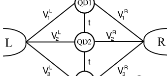
Figure 1: Triple quantum dot molecule coupled in parallel to leads.

The linear conductance at zero temperature is given by the Landauer formula

$$G=\frac{2e^{2}}{h}T(\varepsilon_{F}),$$ (6)

where $T(\omega)$ is the total transmission. To obtain $G$ explicitly we use the equation of motion approach for the Green’s functions.greens The transmission can be expressed in terms of the retarded and advanced Green’s functions $\textbf{G}^{r/a}(\omega)$ as

$$T(\omega)=tr\{\mathbf{G}^{a}(\omega)\mathbf{\Gamma}^{R}\mathbf{G}^{r}(\omega)\mathbf{\Gamma}^{L}\},$$ (7)

where $\mathbf{G}^{r}(\omega)$ is defined by

$$G_{ij}^{r}(t)=-i\theta(t)\langle\{d_{i}(t),d_{j}^{\dagger}(0)\}\rangle,\quad i,j=1,2,3,$$ (8)

with $\theta(t)$ the step function. $\mathbf{G}^{a}(\omega)$ is given by $G_{ij}^{a}=[G_{ji}^{r}]^{*}$, and ${\mathbf{\Gamma}}^{L,R}$ are matrices describing the coupling between the quantum dots and the left and right leads, the matrix elements of which are

$$\Gamma^{L(R)}_{ij}=2\pi\sum_{k}V^{L(R)}_{ik}[V^{L(R)}_{jk}]^{*}\delta(\omega-\omega_{k}),\quad\mbox{$i,j=1,2,3$}.$$ (9)

With the use of Eq. (5), ${\mathbf{\Gamma}}^{L,R}$ can be written as

$${\mathbf{\Gamma}}^{L,R}=\left(\begin{array}[]{lll}\;\;\;\;\gamma_{11}&e^{\mp i\phi/4}\gamma_{12}&e^{\mp i\phi/2}\gamma_{13}\\ e^{\pm i\phi/4}\gamma_{21}&\;\;\;\;\gamma_{22}&e^{\mp i\phi/4}\gamma_{23}\\ e^{\pm i\phi/2}\gamma_{31}&e^{\pm i\phi/4}\gamma_{32}&\;\;\;\;\gamma_{33}\end{array}\right),$$ (10)

with $\gamma_{ij}\equiv\Gamma^{L}_{ij}=\Gamma^{R}_{ij}$, where $\Gamma^{L,R}_{ij}$ are obtained from (9) for zero magnetic flux.

The electronic properties of the configuration can be studied from the total density of states. This quantity is given by

$$\rho(\omega)=\sum_{i=1}^{3}\rho_{i}(\omega)=-\frac{1}{\pi}\sum_{i=1}^{3}{\mbox{I}m}G_{ii}^{r}(\omega),\quad i=1,2,3,$$ (11)

where $G^{r}(\omega)$ is the retarded Green’s function.

Hereafter we assume $\omega_{1}=\omega_{2}=\omega_{3}\equiv\omega_{0}$. We make the following transformation of the quantum-dot operators

$$\bar{d}_{1} = \frac{1}{2}(d_{1}+\sqrt{2}d_{2}+d_{3}),$$

$$\bar{d}_{2} = \frac{1}{\sqrt{2}}(d_{1}-d_{3}),$$

$$\bar{d}_{3} = \frac{1}{2}(d_{1}-\sqrt{2}d_{2}+d_{3}),$$ (12)

so that the Hamiltonian of the isolated molecule becomes diagonal

$$\bar{H}_{m}=(\omega_{0}+\sqrt{2}t)\bar{d}^{\dagger}_{1}\bar{d}_{1}+\omega_{0}\bar{d}_{2}^{\dagger}\bar{d}_{2}+(\omega_{0}-\sqrt{2}t)\bar{d}^{\dagger}_{3}\bar{d}_{3},$$ (13)

and the Hamiltonian describing the coupling between the molecule and the leads takes the form

$$\bar{H}_{I} = \sum_{i=1}^{3}\sum_{k\in L}\bar{V}^{L}_{i}\bar{d}_{i}^{{\dagger}}c_{k}+\mbox{h. c.}+\sum_{i=1}^{3}\sum_{{k}\in R}\bar{V}^{R}_{i}\bar{d}_{i}^{{\dagger}}c_{k}+\mbox{h. c.},$$

where

$$\bar{V}^{L,R}_{1} = \frac{1}{2}({V}^{L,R}_{1}+\sqrt{2}{V}^{L,R}_{2}+{V}^{L,R}_{3}),$$

$$\bar{V}^{L,R}_{2} = \frac{1}{\sqrt{2}}({V}^{L,R}_{1}-{V}^{L,R}_{3}),$$

$$\bar{V}^{L,R}_{3} = \frac{1}{2}({V}^{L,R}_{1}-\sqrt{2}{V}^{L,R}_{2}+{V}^{L,R}_{3}).$$ (15)

Eqs. (5) and (15) give us interesting insight into the transmission properties of the molecule. It is straightforward to see that for some specific values of the magnetic flux and the dot-lead matrix elements, the coupling between one or more molecular states with the leads may vanish, giving rise to the formation of a BIC. In particular, if $V_{1}=V_{3}$,

$$\bar{V}^{L,R}_{1} = 2V_{1}\cos\frac{\phi}{4}+\sqrt{2}V_{2},$$

$$\bar{V}^{L,R}_{2} = \mp i\sqrt{2}V_{1}\sin{\frac{\phi}{4}},$$

$$\bar{V}^{L,R}_{3} = 2V_{1}\cos\frac{\phi}{4}-\sqrt{2}V_{2}.$$ (16)

So that when $\phi=4n\pi$ ($n$ integer), the matrix elements between the molecular state 2 and the left and right leads, $\bar{V}^{L,R}_{2}$, cancel and such a state becomes a BIC. If it also occurs that $V_{1}=V_{2}$, and $n$ is an odd multiple of $\pi$, $\bar{V}^{L,R}_{2}\neq 0$ but either $\bar{V}^{L,R}_{1}$ or $\bar{V}^{L,R}_{3}$ vanish, occurring again a bound state in the continuum. On the other hand, we can see of Eq. (16) that if $V_{1}=V_{3}$ and $V_{2}=\sqrt{2}V_{1}$, two BICs are simultaneously formed when $\phi=4n\pi$: one in the state 2 ($\omega=\omega_{0}$), and other either in state 1 ($\omega=\omega_{0}-\sqrt{2}t$) or 3 ($\omega=\omega_{0}+\sqrt{2}t$), depending on the parity of $n$. In a parallel double quantum dot molecule, a simpler condition gives rise to one BIC, which is formed whenever $\phi$ is a even multiple of $\pi$ (that is, $\Phi=n\Phi_{0}$, $n$ integer).lldg ; orellana Notice that bound states in the continuum occur for numerous combinations of dot-lead couplings and Aharonov-Bohm phases, but, for simplicity, we will restrict our attention to the particular cases: A. $V_{1}=V_{2}=V_{3}\equiv V$ and B. $V_{1}=V_{3}\equiv V$ and $V_{2}=\sqrt{2}V$. The equation of motion method in the molecular basis $\{|\bar{1}\rangle,|\bar{2}\rangle,|\bar{3}\rangle\}$ gives for the retarded Green’s function in both cases

$$\bar{{\mathbf{G}}}^{r}(\omega)=\frac{1}{\Lambda}\left(\begin{array}[]{lll}\sqrt{2}t+\omega+i\bar{\Gamma}_{33}/2&\;\;\;\;0&\;\;\;\;-i\bar{\Gamma}_{13}/2\\ \;\;\;\;0&\Lambda/(\omega+i\bar{\Gamma}_{22}/2)&\;\;\;\;0\\ -i\bar{\Gamma}_{31}/2&\;\;\;\;0&-\sqrt{2}t+\omega+i\bar{\Gamma}_{11}/2\\ \end{array}\right),$$ (17)

where

$$\Lambda=\frac{\bar{\Gamma}_{13}\bar{\Gamma}_{31}}{4}+(-\sqrt{2}t+\omega+i\frac{\bar{\Gamma}_{11}}{2})(\sqrt{2}t+\omega+i\frac{\bar{\Gamma}_{33}}{2}),$$ (18)

with $\bar{\Gamma}_{ij}=\bar{\Gamma}^{L}_{ij}+\bar{\Gamma}^{R}_{ij}$ ($i,j=1,3$), where the matrices $\bar{\mathbf{\Gamma}}^{L}$ and $\bar{\mathbf{\Gamma}}^{R}$ describe the tunneling between the molecular states and the left and right leads, respectively.

III Conductance and density of states

A. $V_{1}=V_{2}=V_{3}$

When $V_{1}=V_{2}=V_{3}\equiv V$, the conductance takes the form

$$G(\omega)=\frac{2e^{2}}{h}\frac{\gamma^{2}[(\omega+2t\cos{\frac{\phi}{4}})^{2}-2(2t^{2}-\omega^{2})\cos{\frac{\phi}{2}}]^{2}}{[\omega^{2}+\gamma^{2}(1-\cos{\frac{\phi}{2}})^{2}][(2t^{2}-\omega^{2})^{2}+\gamma^{2}(4t\cos{\frac{\phi}{4}}+\omega[2+\cos{\frac{\phi}{2}}])^{2}]},$$ (19)

where $\gamma\equiv\Gamma^{L}_{ij}=\Gamma^{R}_{ij}$, for all $i,j=1,2,3$. Figure 2 shows the conductance as a function of the Fermi energy for different values of $\phi$. In general, three resonances are observed around the energies of the molecular states. In Fig. 2(a), where $\phi=0$, the cancellation of the resonance around $\omega=0$ accounts for the existence of the BIC produced when $\phi=4\pi n$ ($n$ integer). The same figure shows $G(\omega)$ for $\phi=\pi/5$, where the resonance corresponding to $\omega=0$ is well resolved. For this value of magnetic flux, as well as for arbitrary values of $\phi$, the conductance displays two Fano antiresonances, at energies

$$\omega=\frac{-\sqrt{2}t(\sqrt{2}\cos{\frac{\phi}{4}}\pm\sqrt{1+\cos\phi})}{1+2\cos{\frac{\phi}{2}}},$$

as follows from Eq. (19). There are some special cases in which the conductance shows only one antiresonance, namely, when $\cos\phi=-1$ (i.e., when $\phi=(2n+1)\pi$, with $n$ integer), and also when $\cos(\phi/2)=-1/2$ (that is, $\phi=2\pi(2n-2/3)$, $n$ integer), where one of the antiresonances goes to infinity and the other keeps in a finite energy. We notice in Figs. 2(b) and (c) (dashed line) that the resonance associated to the bonding state remains very narrow for a wide range of values of $\phi$, approximately from $\phi=-3\pi/2$ to $\phi=3\pi/2$, with a periodicity $8\pi$. In the particular case when $\phi=2\pi(4n+1/2)$ ($n$ integer), for instance in the solid line in (c), the resonance is absent, so that the bonding state is a BIC. This is consistent with Eqs. (16), where $\bar{V}^{L}_{3}$ and $\bar{V}^{R}_{3}$ vanish for these values of $\phi$, leaving such a state decoupled of the leads. In the same figure we included the curve for $\phi=1.2\pi$ (dash line), to show the presence of that resonance again. In (d), where $\phi=2\pi$ ($\Phi=\Phi_{0}$), the conductance is totally symmetric with respect to $\omega=0$. These features repeat whenever $\phi$ is an odd integer of $2\pi$. When $\phi$ is greater than $2\pi$ the conductance spectrum suffers a reflection respect to $\omega=0$, and every $4\pi$ (or two flux quanta) the roles of the bonding and antibonding states are interchanged. Bound states in the continuum are formed in the antibonding state when $\phi=2\pi(4n+3/2)$ ($n$ integer).

Figure 2: Dimensionless conductance versus Fermi energy, in units of $\gamma$, for $V_{1}=V_{2}=V_{3}=V$, $t=2$, a) $\phi=0$ (solid line) and $\phi=\pi/5$ (dash line), b) $\phi=3\pi/4$, c) $\phi=\pi$ (solid line) and $\phi=6\pi/5$ (dash line) d) $\phi=2\pi$, for $\omega_{0}=0$.

Let us now examine the total density of states in the different regimes. This has the form

$$\rho_{T}=\frac{\gamma}{\pi}\left[\frac{8t\omega\cos{\frac{\phi}{4}}+(2t^{2}+\omega^{2})(2+\cos{\frac{\phi}{2}})}{(2t^{2}-\omega^{2})^{2}+\gamma^{2}(4t\cos{\frac{\phi}{4}}+\omega(2+\cos{\frac{\phi}{2}}))^{2}}+\frac{2\sin^{2}{\frac{\phi}{4}}}{\omega^{2}+4\gamma^{2}\sin^{4}{\frac{\phi}{4}}}\right].$$ (20)

Figure 3 shows $\rho_{T}(\omega)$ for the same parameters of Fig. 2. In the curves (a) and (c), where $\phi=0$ and $\phi=\pi$, respectively, the delta functions corresponding to the BICs are observed, superimposed to the peaks associated to the other two molecular states with finite widths.

Figure 3: Density of state versus Fermi energy, in units of $\gamma$, for $V_{1}=V_{2}=V_{3}=V$, $t=2$, a) $\phi=0$, b) $\phi=3\pi/4$, c) $\phi=\pi$ and d) $\phi=2\pi$, and $\omega_{0}=0$

In the approximate range $2(4n-3/4)\pi\leq\phi\leq 2(4n+3/4)\pi$ ($n$ integer) the total density of states can be approximated by the sum of three Lorentzians at the energies $\omega_{-}=-t(8\sqrt{2}t^{2}+4\gamma^{2}\cos(\phi/4)[2+\cos{(\phi/2)}])/(8t^{2}+\gamma^{2}[2+\cos{(\phi/2)}])$, $0$ and $\sqrt{2}t$,

$$\rho_{T}\approx\frac{C}{\pi}\left[\frac{\Gamma_{-}}{\Gamma_{-}^{2}+(\omega-\omega_{-})^{2}}+\frac{\Gamma_{+}}{\Gamma_{+}^{2}+(\omega-\sqrt{2}t)^{2}}\right]+\frac{1}{\pi}\frac{\Gamma_{0}}{\Gamma_{0}^{2}+\omega^{2}},$$ (21)

where

$$\Gamma_{-} = 2\sqrt{2}t^{2}\gamma\frac{-4\cos{\frac{\phi}{4}}+\sqrt{2}[2+\cos{\frac{\phi}{2}}]}{8t^{2}+\gamma^{2}[2+\cos{\frac{\phi}{2}}]^{2}},$$ (22)

$$\Gamma_{0} = 2\gamma\sin^{2}{\frac{\phi}{4}},$$ (23)

$$\Gamma_{+} = \gamma\frac{4\cos{\frac{\phi}{4}}+\sqrt{2}[2+\cos{\frac{\phi}{2}}]}{2\sqrt{2}},$$ (24)

and

$$C=\frac{1}{2}+\frac{\sqrt{2}\cos\frac{\phi}{4}}{2+\cos\frac{\phi}{2}}.$$ (25)

Figure 4 shows the broadenings of the molecular states, $\Gamma_{-}$, $\Gamma_{0}$ and $\Gamma_{+}$, (in units of $\gamma$) as a function of $\phi$, for $t=2$, within the range of validity of the approximations (24). The top curve gives account for the formation of a BIC when $\phi$ is an odd integer of $\pi$, and shows that the corresponding molecular state keeps very slightly coupled to the leads for a wide range of the Aharanov-Bohm phase. In all the interval, $\Gamma_{-}$ keeps smaller than a $7$ per cent of the level broadening of a single dot, and in the interval $(\pi-1/2,\pi+1/2)$ it does not exceed a $1$ per cent. The middle figure shows that the molecular state of intermediate energy ($\omega=0$) is a BIC when $\phi=0$. The width of this molecular state keeps smaller than $1$ for all $\phi\in(-\pi,\pi)$ and is more sensitive to variations of $\phi$ than the one formed in the bonding energy (top figure). However, it is worth to notice that this long-lived state presents for all phases in $(-4\pi/3,4\pi/3)$ larger lifetimes than the long-lived state arising in the parallel-coupled double quantum dot molecule symmetrically connected to leads (where $\Gamma=2\gamma\sin^{2}{\phi/2}$).orellana The behavior of the broadening of the short-lived state is displayed in the bottom plot. This reaches its maximum value (shortest lifetime) when $\phi=0$, where $\Gamma_{+}\approx 2.91$.

Figure 4: Broadenings of the molecular states $\Gamma_{-}$, $\Gamma_{0}$ and $\Gamma_{+}$ as a function of $\phi$, for $V_{1}=V_{2}=V_{3}=V$ and $t=2$.

B. $V_{1}=V_{3}$, $V_{2}=\sqrt{2}V$

Interesting features in the electronic transmission take place when the dot-lead couplings have the form $V_{1}=V_{3}=V$ and $V_{2}=\sqrt{2}V$. Here the linear conductance reduces to

$$G=\frac{2e^{2}}{h}\frac{4\gamma^{2}[(t+\sqrt{2}\omega\cos{\frac{\phi}{4}})^{2}-t^{2}\cos{\frac{\phi}{2}}]^{2}}{[\omega^{2}+\gamma^{2}(1-\cos{\frac{\phi}{2}})^{2}][(2t^{2}-\omega^{2})^{2}+\gamma^{2}(4\sqrt{2}t\cos{\frac{\phi}{4}}+\omega(3+\cos{\frac{\phi}{2}}))^{2}]},$$ (26)

where $\gamma\equiv=\Gamma^{L}_{ij}=\Gamma^{R}_{ij}$, for $i,j=1,3$. Fig. 5 shows the conductance for different values of the Aharonov-Bohm phase. For $\phi=0$ (Fig. 5(a)) this exhibits a single resonance around the antibonding energy, so that the two other molecular states are bound states in the continuum. This also follows of Ecs. (16), since $\bar{V}^{L,R}_{2}$ as well as $\bar{V}^{L,R}_{3}$ cancel whenever $\phi=8n\pi$ ($n$ integer). Also, it can be seen that the roles of the bonding and antibonding states are interchanged every $4\pi$, and that the antibonding and the molecular state of intermediate energy both collapse to BICs when $\phi=4\pi(2n-1)$ ($n$ integer).

Figure 5: Dimensionless conductance versus Fermi energy, in units of $\gamma$, for $V_{1}=V_{3}=V$, $V_{2}=\sqrt{2}V$, $t=2$, a) $\phi=0$ (solid line) and $\phi=\pi/5$ (dash line), b) $\phi=3\pi/4$, c) $\phi=\pi$ (solid line) and $\phi=6\pi/5$ (dash line), d) $\phi=2\pi$, and $\omega_{0}=0$.

For arbitrary values of the Aharonov-Bohm phase the spectrum presents three resonances, and a number of Fano antiresonances that oscillates between two and zero. From Eq. (26) we note that the conductance is zero at

$$\omega=\frac{-\sqrt{2}t[1\pm\sqrt{\cos(\phi/2)}]}{2\cos{\phi/4}},$$ (27)

where we see that when $(4n-1)\pi<\phi<(4n+1)\pi$ ($n$ integer) there are two antiresonaces, as shown by Fig. 5(b) where $\phi=3\pi/4$. When $\phi=n\pi$ ($n$ odd) only one point of zero conductance exists, as observed in (c). For $(4n-3)\pi<\phi<(4n-1)\pi$ ($n$ integer) the numerator of Eq. (26) is complex and the conductance does not exhibit antiresonances (Figs. (c), dashed line, and (d)). In (d) $G(\omega)$ is symmetrical around $\omega=0$, and has the form

$$G=\frac{2e^{2}}{h}\frac{16\gamma^{2}t^{4}}{(4\gamma^{2}+\omega^{2})(4t^{4}-4(t+\gamma)(t-\gamma)\omega^{2}+\omega^{4})},$$

which corresponds exactly to the conductance of a triple quantum dot molecule connected in series.zeng It is interesting to note that if the dots are not coupled directly, that is, $t=0$, the transmission is suppressed for all energies (perfect reflector). An analogous result is found in two parallel quantum dots in presence of a magnetic field.kubala This situation never occurs in the triple molecule when the dot-lead couplings are equal.

The total density of states is given by

$$\rho_{T}(\omega)=\frac{\gamma}{\pi}\left[\frac{8\sqrt{2}t\omega\cos{\frac{\phi}{4}}+(2t^{2}+\omega^{2})(3+\cos{\frac{\phi}{2}})}{(2t^{2}-\omega^{2})^{2}+\gamma^{2}[4\sqrt{2}t\cos{\frac{\phi}{4}}+\omega(3+\cos{\frac{\phi}{2}})]^{2}}+\frac{2\sin^{2}{\frac{\phi}{4}}}{\omega^{2}+4\gamma^{2}\sin^{4}{\frac{\phi}{4}}}\right].$$ (28)

In the range $2(4n-3/8)\pi\leq\phi\leq 2(4n+3/8)\pi$ ($n$ integer), $\rho_{T}$ can be approximated by a sum of Lorentzians of the form Eq. (21), where $\omega_{-}=-4\sqrt{2}t(2t^{2}+\gamma^{2}\cos(\phi/4)[3+\cos{(\phi/2)}])/(8t^{2}+\gamma^{2}[3+\cos(\phi/2)]^{2})$,

$$C=\frac{4\cos^{4}{\frac{\phi}{4}}}{3+\cos\frac{\phi}{2}}$$ (29)

and the broadenings are given by

$$\Gamma_{-} = 8\gamma\frac{t^{2}\sin^{4}{\frac{\phi}{8}}}{2t^{2}+\gamma^{2}(1+\cos^{2}{\frac{\phi}{4}})^{2}}$$ (30)

$$\Gamma_{0} = 2\gamma\sin^{2}\frac{\phi}{4}$$ (31)

$$\Gamma_{+} = 4\gamma\cos^{4}{\frac{\phi}{8}}$$ (32)

Figure 6: Density of state versus Fermi energy, in units of $\gamma$, for $V_{1}=V_{3}=V$, $V_{2}=\sqrt{2}V$, $t=2$, a) $\phi=0$, b) $\phi=3\pi/4$, c) $\phi=\pi$ and d) $\phi=2\pi$, for $\omega_{0}=0$.

Fig. 6 shows $\rho_{T}$ for the same parameters of Fig.5. In figure Fig.6(a), where $\phi=0$, the density of states is the superposition of two Dirac delta’s localized at $\omega=\omega_{-}$ and $\omega=0$ (corresponding to the BICs) plus a Lorentzian at $\omega=\omega_{+}$ with width $4\gamma$. When $\phi=2\pi$, as in (d), the density of states correspond to that of a triple molecule connected in series.

Figure 7: Broadenings of the molecular states $\Gamma_{-}$, $\Gamma_{0}$ and $\Gamma_{+}$ as a function of $\phi$, for $V_{1}=V_{3}=V$, $V_{2}=\sqrt{2}V$ and $t=2$.

Fig. 7 displays the broadenings $\Gamma_{-}$, $\Gamma_{0}$ and $\Gamma_{+}$ as a function of $\phi$, for $t=2$, in the range of validity of Eqs. (32). In the top plot shows the BIC formed in the bonding state when $\phi=0$ and the robustness of the such a long-lived state against variations of the magnetic field. Notice that $\Gamma_{-}$ remains smaller than $0.02$ in all the plotted range of $\phi$, and that is very close to zero in a wide interval around $\phi=0$. For instance, for $\phi\in(-\pi/3,\pi/3)$, $\Gamma_{-}$ keeps smaller than $8\times 10^{-4}$, that is, less than $0.08$ per cent of the level broadening of a single quantum dot. The broadening $\Gamma_{0}$ (which coincide with $\Gamma_{0}$ in the previous setting) is more sensitive to variations of the magnetic field than $\Gamma_{-}$, as shown in the middle figure.

The robustness of the molecular states for the triple quantum dot molecule can be understood physically as follows: in the triple molecule the phases acquired by the electron in covering some of the paths, namely, those containing the central quantum dot, are smaller than those gained when the electron travel though paths containing the outer dots. For instance, along the central path the electron does not accumulate any phase. This information is contained in the effective couplings of the molecular states with the leads, and therefore their dependence on the Aharonov-Bohm phase is less sensitive in comparison to the double quantum dot case.

We interpret the formation of BICs in this system in the same sense of reference [friedrich, ], that is, as result of the quantum interference between resonances of different channels through the multiple connected quantum dots. The levels of the quantum dots are hybridized through the common leads, forming these states of infinite lifetimes. In a more realistic model on transmission through the quantum dot molecule one should take into account the electron-electron interaction. In recent works some authors have found results that can be interpreted as BICs that survive to the interaction effects. For instance, Ding et al.ding study a parallel double quantum dot in the Kondo regime by using the finite-U slave boson technique, and found a $\delta$-peak structure in the density of state for the energies inside the band, signal of a bound state in the continuum. On the another hand, Busser et al.busser study the transport properties of multilevel quantum dots in Kondo regime and report the formation of localized states. We interpret these results as BICs in the same sense described in the present paper. However, we think that the above results are not conclusive and further research is necessary to know the effect of the electron-electron interaction on the formation of BICs.

IV Larger molecules

It is natural to ask about the existence of bound states in the continuum in molecules of $N$ quantum dots, with $N$ arbitrary. As seen for the doublelldg and triple parallel-coupled molecules, the existence a magnetic field is not essential for the formation of BICs , but it is needed just a certain relation of symmetry between the couplings between dots and leads for these to take place. In fact, the maximum number of simultaneous bound states may occur when the magnetic flux is zero. So, a first approach to the problem of a parallel-coupled molecule of $N$ quantum dots can be obtained by assuming that there is no field present.

The $j$-th component of the eigenfunction $|\psi_{n}\rangle$ of a linear chain consisting of $N$ identical quantum dots with energies $\varepsilon_{0}$ and tunnel coupling between dots $t$ is given by

$$\psi_{j,n}=\sqrt{\frac{2}{N+1}}\sin{\frac{jn\pi}{N+1}},\quad j=1,2,\dots,N$$ (33)

and the corresponding eigenenergy is

$$E_{n}=\varepsilon_{0}-2t\cos{\frac{n\pi}{N+1}}.$$ (34)

The Hamiltonian describing the molecule-leads interaction is

$$H_{i}=\sum_{i=1}^{N}\sum_{k\in L}(V_{i}d^{{\dagger}}_{i}c_{k}+\mbox{ h.c.})+\sum_{i=1}^{N}\sum_{k\in R}(V_{i}d^{{\dagger}}_{i}c_{k}+\mbox{ h.c.})$$ (35)

where we have assumed that $V^{L}_{i}=V^{R}_{i}\equiv V_{i}$, for all $i=1,2,\dots,N$. To search for conditions for the formation of BICs, we look at the couplings of the molecular states with the leads, $\bar{V}_{n}$ ($n=1,2,\dots,N$). These can be obtained by the transformation

$$\mathbf{\bar{V}}=P\mathbf{V},$$ (36)

where $\mathbf{\bar{V}}$ y $\mathbf{V}$ are column vectors with elements $\bar{V}_{n}$ and $V_{n}$ ($n=1,2,\dots,N$), respectively, and $P$ is the matrix composed of eigenvectors $|\psi_{n}\rangle$ ($n=1,2,\dots,N$), which components are given by (33). Namely,

$$P=\sqrt{\frac{2}{N+1}}\left(\begin{array}[]{ccccc}\sin{\frac{\pi}{N+1}}&\sin{\frac{2\pi}{N+1}}&\sin{\frac{3\pi}{N+1}}&\cdots&\sin{\frac{N\pi}{N+1}}\\ \sin{\frac{2\pi}{N+1}}&\sin{\frac{4\pi}{N+1}}&\sin{\frac{6\pi}{N+1}}&\cdots&\sin{\frac{2N\pi}{N+1}}\\ \vdots&\vdots&\vdots&\ddots&\vdots\\ \sin{\frac{N\pi}{N+1}}&\sin{\frac{2N\pi}{N+1}}&\sin{\frac{3N\pi}{N+1}}&\cdots&\sin{\frac{N^{2}\pi}{N+1}}\end{array}\right).$$ (37)

It is direct to show that the matrix elements of $P$ have the following properties:

$$P_{i,j} = P_{i,N-j+1}\quad\mbox{$i$ odd}$$ (38)

$$P_{i,j} = -P_{i,N-j+1}\quad\mbox{$i$ even}$$ (39)

$$P_{i,(N+1)/2} = 0,\quad\mbox{$N$ odd and $i$ even}$$ (40)

These relations, together with Eq. (36), allow us to get information on some symmetries leading to the formation of BICs. For instance, if there is up-down symmetry, that is,

$$V_{i}=V_{N-i+1},\quad\mbox{$i=1,2,\cdots,N$},$$

then by the condition (39),

$$\bar{V}_{j}=0,\quad\mbox{for all $j$ even}.$$

Thus, if $N$ is even, $N/2$ bound states in the continuum are ensured. In turn, if $N$ is odd, both conditions (39) and (40) are simultaneously required for the formation of $(N-1)/2$ bound states in the continuum.

We illustrate the above analysis by considering in detail the cases $N=4$ and $N=5$. We get conditions for the formation of additional BICs in each example. For the molecule of four quantum dots, Eqn. (36) reduces to

$$\bar{V}_{1} = \alpha_{+}(V_{2}+V_{3})+\alpha_{-}(V_{1}+V_{4})$$

$$\bar{V}_{2} = \alpha_{-}(V_{2}-V_{3})+\alpha_{+}(V_{1}-V_{4})$$

$$\bar{V}_{3} = -\alpha_{-}(V_{2}+V_{3})+\alpha_{+}(V_{1}+V_{4})$$

$$\bar{V}_{4} = -\alpha_{+}(V_{2}-V_{3})+\alpha_{-}(V_{1}-V_{4}),$$ (41)

where $\alpha_{\pm}=(1/2)\sqrt{1\pm 1/\sqrt{5}}$. We see that if $V_{1}=V_{4}$ and $V_{2}=V_{3}$ both $\bar{V}_{2}$ and $\bar{V}_{4}$ are canceled, thus occurring two BICs. We notice that if also $\alpha_{+}V_{2}=\mp\alpha_{-}V_{1}$, either $\bar{V}_{1}$ or $\bar{V}_{3}$ vanishes, having three of the four molecular states decoupled from the continuum.

For a molecule of five quantum dots we have

$$\bar{V}_{1} = \frac{1}{2}[V_{2}+V_{4}+\frac{\sqrt{3}}{3}(V_{1}+2V_{3}+V_{5})]$$

$$\bar{V}_{2} = \frac{1}{2}(V_{1}+V_{2}-V_{4}-V_{5})$$

$$\bar{V}_{3} = \frac{\sqrt{3}}{3}(V_{1}-V_{3}+V_{5})$$

$$\bar{V}_{4} = \frac{1}{2}(V_{1}-V_{2}+V_{4}-V_{5})$$

$$\bar{V}_{5} = \frac{1}{2}[-(V_{2}+V_{4})+\frac{\sqrt{3}}{3}(V_{1}+2V_{3}+V_{5})].$$ (42)

Because of condition (40) neither $\bar{V}_{2}$ nor $\bar{V}_{4}$ depends on $V_{3}$. This, together with $V_{1}=V_{5}$ and $V_{2}=V_{4}$ lead to the occurrence BICs in the molecular states 2 and 3. Up to two new bound states may arise if the following conditions are met: $V_{3}=2V_{1}$ suppresses $\bar{V}_{3}$ and this together with $V_{2}=\mp V_{1}$ cancel either $\bar{V}_{1}$ or $\bar{V}_{5}$.

V Conclusions

We have investigated electron transport through a parallel-coupled triple quantum dot molecule in presence of a magnetic field. The conductance spectrum exhibits a Breit-Wigner and two Fano resonances, which positions and widths are controlled by the magnetic field. Every two flux quanta ($\phi=4\pi$), the roles of the bonding and antibonding states are interchanged. We have examined the dependence and broadenings of the molecular states as a function of the magnetic flux for two different sets of parameters, finding that several regimes of transmission are possible, including the formation of extremely narrow resonances and bound states in the continuum. We have shown that by manipulating the symmetries of the system, up to two simultaneous BICs can be formed. We restricted our analysis to systems with up-down and left-right symmetries. In Ref. lldg, it is shown that the breaking of the first of those symmetries hinders the formation of BICs, but states of very long lifetimes still occur. With respect to the left-right symmetry, this is not essential in the existence of BICs, as demonstrated in Ref. orellana, for the double quantum dot molecule. We extended the study to molecules of $N$ quantum dots in the absence of magnetic field, finding that the up-down symmetry ensures the occurrence of $N/2$ BICs for $N$ even, and of $(N-1)/2$ for $N$ odd. Additional conditions are required for the existence of a larger number of simultaneous bound states in the continuum, as shown for molecules of four and five dots. In both cases up to $N-1$ BICs may exist at the same time, $N$ being the number of dots.

The possibility of having molecular states decoupled from the leads, and the fact that these states are controllable by an external magnetic field and gate potentials, are interesting features of the studied system which might be useful to classical information theory. Two orthogonal stable states of the molecule, that is, two simultaneous BICs, could be used as microscopic units for storing information (classical bits). Storage of quantum information requires a complete stable plane in the Hilbert space of the molecule.nielsen Quantum dot molecules seem to be suitable systems to study BICs experimentally, because of the possibility of controlling parameters. In fact, other quantum interference phenomena have been demonstrated in this kind of systems, such as Fanokobayashi and Aharonov-Bohmyacobi effects.

References

- (1) M. A. Kastner, Phys. Today 46 24 (1993); R. C. Ashoori, Nature 379, 413 (1996); S. Tarucha, D. G. Austing, T. Honda, R. J. van der Hage, and L. P. Kouwenhoven, Phys. Rev. Lett. 77, 3613 (1996).
- (2) R. H. Blick, D. Pfannkuche, R. J. Haug, K. v. Klitzing, and K. Eberl, Phys. Rev. Lett. 80, 4032 (1998).
- (3) R. Ziegler, C. Bruder, and Herbert Schoeller, Phys. Rev. B 62, 1961 (2000).
- (4) W. G. van der Wiel, S. De Franceschi, J. M. Elzerman, T. Fujisawa, S. Tarucha, and L. P. Kouwenhoven, Rev. Mod. Phys. 75, 1-22 (2003).
- (5) Vitaly N. Golovach and Daniel Loss, Phys. Rev. B, 69, 245327 (2004).
- (6) F. R. Waugh, M. J. Berry, D. J. Mar, and R. M. Westervelt, K. L. Campman, and A. C. Gossard, Phys. Rev. Lett. 75 705 (1995).
- (7) F. R. Waugh, M. J. Berry, C. H. Crouch, C. Livermore, D. J. Mar, R. M. Westervelt, K. L. Campman, and A. C. Gossard, Phys. Rev. B, 53, 1413 (1996).
- (8) L. P. Kouwenhoven, F. W. J. Hekking, B. J. van Wees, C. J. P. M. Harmans, C. E. Timmering, and C. T. Foxon, Phys. Rev. Lett. 65, 361 (1990).
- (9) Z. Y. Zeng and F. Claro, Phys. Rev. B 65 193405 (2002).
- (10) Kicheon Kang, Phys. Rev. B 59, 4608 (1999).
- (11) J. Göres, D. Goldhaber-Gordon, S. Heemeyer, M. A. Kastner, H. Shtrikman, D. Mahalu, and U. Meirav, Phys. Rev. B 62, 2188 (2000).
- (12) Kensuke Kobayashi, Hisashi Aikawa, Shingo Katsumoto, and Yasuhiro Iye, Phys. Rev. Lett. 88, 256806 (2002).
- (13) U. Fano, Phys. Rev. 124, 1866 (1961).
- (14) Björn Kubala and Jürgen König, Phys. Rev. B 65, 245301 (2002).
- (15) Kicheon Kang and Sam Young Cho, J. Phys: Condens. Matter 16, 117 (2004).
- (16) Zhi-Ming Bai, Min-Fong Yang, and Yung-Chung Chen, J. Phys.: Condens. Matter 16, 2053 (2004).
- (17) Pedro A. Orellana, M. L. Ladrón de Guevara, and F. Claro Phys. Rev. B 70, 233315 (2004).
- (18) V. Moldoveanu, M. Tolea, A. Aldea, and B. Tanatar, Phys. Rev. B 71, 125338 (2005).
- (19) Haizhou Lu, Rong Lü, and Bang-fen Zhu, Phys. Rev. B 71, 235320 (2005).
- (20) M. L. Ladrón de Guevara, F. Claro, and Pedro A. Orellana, Phys. Rev. B 67, 195335 (2003).
- (21) J. von Neumann and E. Wigner, Phys. Z. 30, 465 (1929).
- (22) Frank H. Stillinger and David R. Herrick, Phys. Rev. A 11, 446 (1975).
- (23) H. Friedrich and D. Wintgen, Phys. Rev. A 31, 3964 (1985); H. Friedrich and D. Wintgen, Phys. Rev. A 32, 3231 (1985).
- (24) R. L. Schult, H. W. Wyld, and D. G. Ravenhall, Phys. Rev. B 41, 12760 (1990).
- (25) Zhen-Li Ji and Karl-Frederik Berggren, Phys. Rev. B 45, 6652 (1992).
- (26) Federico Capasso, Carlo Sirtori, Jerome Faist, Deborah L. Sivico, Sung-Nee G. Chu and Alfred Y. Cho, Nature 358, 565 (1992).
- (27) J. U. Nöckel, Phys. Rev. B 46 15348 (1992).
- (28) O. Olendski and L. Mikhailovska, Phys. Rev B 67, 035310 (2003).
- (29) I. Rotter and A. F. Sadreev, Phys. Rev. E 71, 046204 (2005).
- (30) Guo-Hui Ding, Chul Koo Kim, and Kyun Nahm, Phys. Rev. B, 71 205313 (2005).
- (31) C. A. Busser, G. B. Martins, K. A. Al-Hassanieh, Adriana Moreo, and Ebio Dagotto, Phys. Rev. B 70, 245303 (2004).
- (32) Supriyo Datta, “Electronic transport in mesoscopic systems” (Cambridge Univ. Press, 1997).
- (33) M. A. Nielsen and I. L. Chuang, Quantum Computation and Quantum Information (Cambridge University Press, Cambridge, U.K., 2000).
- (34) A. Yacoby, M. Heiblum, D. Mahalu, and H. Shtrikman, Phys. Rev. Lett. 74, 4047 (1995).