Spectral functions of the spinless Holstein model

Abstract

An analytical approach to the one-dimensional spinless Holstein model is proposed, which is valid at finite charge-carrier concentrations. Spectral functions of charge carriers are computed on the basis of self-energy calculations. A generalization of the Lang-Firsov canonical transformation method is shown to provide an interpolation scheme between the extreme weak– and strong-coupling cases. The transformation depends on a variationally determined parameter that characterizes the charge distribution across the polaron volume. The relation between the spectral functions of polarons and electrons, the latter corresponding to the photoemission spectrum, is derived. Particular attention is paid to the distinction between the coherent and incoherent parts of the spectra, and their evolution as a function of band filling and model parameters. Results are discussed and compared with recent numerical calculations for the many-polaron problem.

1 Introduction

Experiments on a variety of novel materials, ranging from quasi-one-dimensional (1D) MX solids [1], organics [2] and quasi-2D high-$T_{\rm c}$ cuprates [3] to 3D colossal-magnetoresistive manganites [4, 5], provide clear evidence for the existence of polaronic carriers, i.e., quasiparticles consisting of an electron and a surrounding lattice distortion. This has motivated considerable theoretical efforts to achieve a better understanding of strongly coupled electron-phonon systems in the framework of microscopic models.

Unfortunately, even for highly simplified models, such as the spinless Holstein model [6] considered here, no exact analytical solutions exist, except for the Holstein polaron problem with a relativistic dispersion [7] or in infinite dimensions [8]. As a consequence, numerous numerical studies have been carried out, focussing either on the empty band limit (i.e., one or two electrons only; see [10, 11, 12, 13, 15] and references therein), or on the half-filled band case in one dimension, where the Peierls transition takes place [16]. In contrast, very little work has been done at finite carrier densities away from half filling [20, 22], which are, however, often realized in experiment [1, 2, 3, 4, 5]. Recently, this so-called many-polaron problem has been addressed numerically [23, 24, 25]. The results have led to a fairly good understanding of many aspects, but their interpretation is not always straight forward, which makes analytical calculations along these lines highly desirable.

In this paper, we propose an analytical approach to the 1D spinless Holstein model, capable of describing finite charge-carrier concentrations at arbitrary model parameters, including the important adiabatic intermediate-coupling (IC) regime.

First, using standard perturbation theory based on the self-energy calculation, the spectral functions of charge carriers will be determined in the weak-coupling (WC) and the strong-coupling (SC) limits at zero temperature ($T=0$). In the SC regime, the relation between the spectral function of polarons, determining the equilibrium properties (in particular, the chemical potential), and the electronic spectral function, determining the photoemission spectrum, will be discussed. Special emphasis will be laid on the distinction between the coherent and the incoherent parts of the spectra, which may be calculated separately within the present approach.

Furthermore, using a generalization of the Lang-Firsov canonical transformation method [27], an interpolation scheme between the extreme WC and SC cases will be proposed. In particular, the canonical transformation will depend on the distance $R$ characterizing the charge distribution across the polaron volume. For a given set of model parameters and carrier concentration $n$, $R$ will be determined from the minimum of the total energy given by the transformed Hamiltonian in the first, Hartree-like approximation. With $R$ found in this way, the polaronic and electronic spectral functions will be calculated to study their dependence on the model parameters and the carrier density. The results will be discussed with regard to recent numerical calculations [24, 25], which have revealed a cross-over from a system with polaronic carriers to a rather metallic system with increasing band filling $n$ in the intermediate electron-phonon coupling regime.

The paper is organized as follows. In section 2.1 we introduce the model used, whereas in section 2.2 we derive the analytical results for WC, SC and IC regimes. Our results are discussed in section 3, and section 4 contains our conclusions.

2 Theory

2.1 Model

In this paper, we are exclusively concerned with the Holstein model (HM) of spinless fermions, which describes electrons coupled locally to Einstein phonons. Although we shall use different canonical transformations to describe the IC and SC regime later on, the Hamiltonian can be written in the general form

$$H=\eta\sum_{i}c^{\dagger}_{i}c^{\phantom{{\dagger}}}_{i}-\sum_{i,j}C_{ij}^{\phantom{{\dagger}}}c_{i}^{{\dagger}}c_{j}^{\phantom{{\dagger}}}+\omega_{0}\sum_{i}(b_{i}^{{\dagger}}b_{i}^{\phantom{{\dagger}}}+\mbox{\small$\frac{1}{2}$})\,,$$ (1)

where the definition of $\eta$ and $C_{ij}$ will be different depending on the approach used. Here $c_{i}^{{\dagger}}$ ($c_{i}^{\phantom{{\dagger}}}$) creates (annihilates) a spinless fermion at site $i$, $b_{i}^{{\dagger}}$ and $b_{i}^{\phantom{{\dagger}}}$ are bosonic operators for the dispersionless phonons of energy $\omega_{0}$ ($\hbar=1$), and the strength of the electron-phonon interaction is specified by the dimensionless coupling constants $\lambda=E_{\mathrm{p}}/2t$ and $g=\sqrt{E_{\mathrm{p}}/\omega_{0}}$ in the adiabatic ($\omega_{0}/t\ll 1$) and anti-adiabatic ($\omega_{0}/t\gg 1$) regimes, respectively, where $E_{\mathrm{p}}$ is the well-known polaron binding energy in the atomic limit [$C_{ij}=0$ for $i\neq j$ in equation (1)].

In the WC case, in which we use the original, untransformed Holstein Hamiltonian, we have $\eta=-\mu$, where $\mu$ denotes the chemical potential, and non-zero coefficients

$$C_{ii}=g\omega_{0}(b_{i}^{{\dagger}}+b_{i}^{\phantom{{\dagger}}})\,,\qquad C_{\langle ij\rangle}=t\,.$$ (2)

In contrast, the starting point in the SC regime will be the Hamiltonian with $\eta=-g^{2}\omega_{0}-\mu=-E_{\mathrm{p}}-\mu$ and

$$C_{ii}=0\,,\qquad C_{\langle ij\rangle}=t\rme^{-g(b_{i}^{{\dagger}}-b_{i}^{\phantom{{\dagger}}}-b_{j}^{{\dagger}}+b_{j}^{\phantom{{\dagger}}})}\,.$$ (3)

2.2 Green functions approach

We treat the HM (1) using the formalism of the generalized Matsubara Green functions introduced by Kadanoff and Baym [28] and Bonch-Bruevich and Tyablikov [29], and applied to the single-polaron problem by Schnakenberg [30]. The Green function equation of motion deduced from $H$ may be converted into an equation for the self-energy of the spinless fermions, and can be solved by iteration (see [30, 31, 32] for details). In the second iteration step, the self-energy is obtained in the form

$$\Sigma(j_{1}\tau_{1};j_{2}\tau_{2})=-\langle C_{j_{1}j_{2}}\rangle\delta(\tau_{1}-\tau_{2})$$

$$+\sum_{j^{\prime}j^{\prime\prime}}G^{\mathrm{M}}(j^{\prime}\tau_{1};j^{\prime\prime}\tau_{2})[\langle T_{\tau}C_{j_{1}j^{\prime}}(\tau_{1})C_{j^{\prime\prime}j_{2}}(\tau_{2})\rangle-\langle C_{j_{1}j^{\prime}}\rangle\langle C_{j^{\prime\prime}j_{2}}\rangle]\,,$$ (4)

where $G^{\mathrm{M}}(j_{1}\tau_{1};j_{2}\tau_{2})$ represents the first-order fermionic Matsubara Green function, and the symbol $T_{\tau}$ denotes the time ordering operator acting on the imaginary times $\tau_{i}$. Fourier-transforming both sides of equation (2.2), carrying out the standard summation over the Matsubara boson frequencies [33], and using the analytical continuation in the complex frequency plane, the retarded momentum– and energy-dependent fermion Green function follows as

$$G^{\mathrm{R}}(k,\overline{\omega})=\frac{1}{\overline{\omega}-(\xi_{k}+\eta)-\Sigma(k,\overline{\omega})}\,,$$ (5)

where $\xi_{k}$ is the fermionic band dispersion in the first approximation, $\overline{\omega}=\omega+\rmi\epsilon$ ($\epsilon\rightarrow 0^{+}$), and $\Sigma(k,\omega)$ denotes the Fourier transform of the collisional part of the self-energy given by the second term on the r. h. s of equation (2.2). The related, normalized spectral function is given by

$$A(k,\omega)=-\frac{1}{\pi}\mathrm{Im}\,G^{\mathrm{R}}(k,\omega+\rmi 0^{+})\,.$$ (6)

Although the insulating Peierls phase with long-range charge-density-wave order, which is the ground state of the half-filled spinless Holstein model above a critical coupling strength depending on $\omega_{0}$ [16], can in principle be incorporated into the present theory, this has not been done here, as we are interested in intermediate band fillings away from $n=0.5$. Furthermore, we neglect any extended pairing for $0<n<0.5$, as well as the possible formation of a polaronic superlattice in the half-filled band case ($n=0.5$). Finally, the possibility of phase separation, which can in principle occur in the present model, is not considered.

2.2.1 Weak coupling

In the WC limit the self-energy is given by

$$\Sigma(k,\overline{\omega})=\frac{\omega_{0}E_{\mathrm{p}}}{\pi W}\int_{-W}^{W}\frac{\rmd\xi}{\sqrt{1-(\xi/W)^{2}}}\left[\frac{1-n_{\mathrm{F}}(\xi-\mu)}{\overline{\omega}-\omega_{0}-(\xi-\mu)}+\frac{n_{\mathrm{F}}(\xi-\mu)}{\overline{\omega}+\omega_{0}-(\xi-\mu)}\right]\,,$$ (7)

with the Fermi function $n_{\mathrm{F}}(\omega)=(\rme^{\beta\omega}+1)^{-1}$ and the bare bandwidth $W=2t$. At $T=0$, and defining $\xi_{0}=\max{(\mu,-W)}$, we get

$$\mathrm{Re}\,\Sigma(k,\omega)=\frac{\omega_{0}E_{\mathrm{p}}}{\pi W}\left[\mathcal{P}\int_{-W}^{\xi_{0}}\frac{\rmd\xi}{\sqrt{1-(\xi/W)^{2}}}\frac{1}{\omega+\omega_{0}-(\xi-\mu)}\right.$$

$$+\left.\mathcal{P}\int_{\xi_{0}}^{W}\frac{\rmd\xi}{\sqrt{1-(\xi/W)^{2}}}\frac{1}{\omega-\omega_{0}-(\xi-\mu)}\right]$$ (8)

and

$$\mathrm{Im}\,\Sigma(k,\omega)=-\frac{\omega_{0}E_{\mathrm{p}}}{W}\left[\int_{-W}^{\xi_{0}}\frac{\rmd\xi}{\sqrt{1-(\xi/W)^{2}}}\delta[\omega+\omega_{0}-(\xi-\mu)]\right.$$

$$+\left.\int_{\xi_{0}}^{W}\frac{\rmd\xi}{\sqrt{1-(\xi/W)^{2}}}\delta[\omega-\omega_{0}-(\xi-\mu)]\right]\,.$$ (9)

In the sequel, we shall distinguish between coherent and incoherent contributions to the single-particle spectral functions, as defined by a zero and non-zero imaginary part of the self-energy, respectively. The coherent part of the spectrum is given by

$$A^{\mathrm{c}}(k,\omega)=z_{k}\delta[\omega-(E_{k}-\mu)]\,,$$ (10)

where the renormalized band energy is the solution of

$$E_{k}=\xi_{k}+\frac{\omega_{0}E_{\mathrm{p}}}{\pi W}\left[\mathcal{P}\int_{-W}^{\xi_{0}}\frac{\rmd\xi}{\sqrt{1-(\xi/W)^{2}}}\frac{1}{E_{k}+\omega_{0}-\xi}\right.$$

$$+\left.\mathcal{P}\int_{\xi_{0}}^{W}\frac{\rmd\xi}{\sqrt{1-(\xi/W)^{2}}}\frac{1}{E_{k}-\omega_{0}-\xi}\right]\,,$$ (11)

with $\xi_{k}=-W\cos{k}$ (the bare band dispersion), and the spectral weight takes the form

$$z_{k}^{-1}=\bigg{|}1+\frac{\omega_{0}E_{\mathrm{p}}}{\pi W}\left[\mathcal{P}\int_{-W}^{\xi_{0}}\frac{\rmd\xi}{\sqrt{1-(\xi/W)^{2}}}\frac{1}{(E_{k}+\omega_{0}-\xi)^{2}}\right.$$

$$+\left.\mathcal{P}\int_{\xi_{0}}^{W}\frac{\rmd\xi}{\sqrt{1-(\xi/W)^{2}}}\frac{1}{(E_{k}-\omega_{0}-\xi)^{2}}\right]\bigg{|}\,.$$ (12)

For the incoherent part of the spectral function we find

$$A^{\mathrm{ic}}(k,\omega<-\omega_{0})=\frac{1}{\pi}\frac{\omega_{0}E_{\mathrm{p}}\left[W^{2}-(\omega+\omega_{0}+\mu)^{2}\right]^{\frac{1}{2}}\int_{-W}^{\xi_{0}}\rmd\xi\delta(\omega+\omega_{0}+\mu-\xi)}{\left[W^{2}-(\omega+\omega_{0}+\mu)^{2}\right]\left(\omega+\mu-\xi_{k}-\mathrm{Re}\,\Sigma(k,\omega)\right)^{2}+(\omega_{0}E_{\mathrm{p}})^{2}}$$ (13)

and

$$A^{\mathrm{ic}}(k,\omega>\omega_{0})=\frac{1}{\pi}\frac{\omega_{0}E_{\mathrm{p}}\left[W^{2}-(\omega-\omega_{0}+\mu)^{2}\right]^{\frac{1}{2}}\int_{\xi_{0}}^{W}\rmd\xi\delta(\omega-\omega_{0}+\mu-\xi)}{\left[W^{2}-(\omega-\omega_{0}+\mu)^{2}\right]\left(\omega+\mu-\xi_{k}-\mathrm{Re}\,\Sigma(k,\omega)\right)^{2}+(\omega_{0}E_{\mathrm{p}})^{2}}\,.$$ (14)

Finally, the chemical potential $\mu$ for a given electron density $n$ is determined by

$$\frac{1}{N}\sum_{k}\int_{-\infty}^{\infty}\rmd\omega A(k,\omega)n_{\mathrm{F}}(\omega)=n\,.$$ (15)

2.2.2 Strong coupling

Hamiltonian (1) with the coefficients (3) represents the Hamiltonian of small polarons, which are the correct quasiparticles in the SC limit. Using the procedure outlined above, we obtain the polaron self-energy as

$$\Sigma(k,\overline{\omega})=\frac{\widetilde{W}}{2\pi}\sum_{s\geq 1}\int_{-\widetilde{W}}^{\widetilde{W}}\frac{\rmd\xi f(k,\xi,s)}{\sqrt{1-(\xi/\widetilde{W})^{2}}}\left[\frac{1-n_{\mathrm{F}}(\xi+\eta)}{\overline{\omega}-s\omega_{0}-(\xi+\eta)}+\frac{n_{\mathrm{F}}(\xi+\eta)}{\overline{\omega}+s\omega_{0}-(\xi+\eta)}\right]\,.$$ (16)

At $T=0$, we have $\widetilde{W}=W\rme^{-g^{2}}$,

$$\mathrm{Re}\,\Sigma(k,\omega)=\frac{\widetilde{W}}{2\pi}\sum_{s\geq 1}\mathcal{P}\int_{-\widetilde{W}}^{\widetilde{W}}\frac{\rmd\xi}{\sqrt{1-(\xi/\widetilde{W})^{2}}}f(k,\xi,s)$$

$$\times\left[\frac{\theta(\xi+\eta)}{\omega-s\omega_{0}-(\xi+\eta)}+\frac{\theta(-\xi-\eta)}{\omega+s\omega_{0}-(\xi+\eta)}\right]$$ (17)

and

$$\mathrm{Im}\,\Sigma(k,\omega)=-\frac{\widetilde{W}}{2}\sum_{s\geq 1}\int_{-\widetilde{W}}^{\widetilde{W}}\frac{\rmd\xi}{\sqrt{1-(\xi/\widetilde{W})^{2}}}f(k,\xi,s)\left\{\theta(\omega-s\omega_{0})\delta[\omega-s\omega_{0}-(\xi+\eta)]\right.$$

$$\left.+\theta(-\omega-s\omega_{0})\delta[\omega+s\omega_{0}-(\xi+\eta)]\right\}\,.$$ (18)

Here $\theta(x)$ is the Heaviside step function and we have used the definition

$$f(k,\xi,s)=\frac{(2g^{2})^{s}}{s!}+\frac{(g^{2})^{s}}{s!}\left[2\left(\frac{\xi}{\widetilde{W}}\right)^{2}-1\right]+\frac{(g^{2})^{s}}{s!}\cos(2k)\,.$$ (19)

The coherent part of the spectrum, non-zero for $|\omega|<\omega_{0}$, is given by

$$A^{\mathrm{c}}(k,\omega)=z_{k}\delta[\omega-(E_{k}+\eta)]$$ (20)

with the renormalized band energy $E_{k}$ being the solution of

$$E_{k}=\xi_{k}+\mathrm{Re}\,\Sigma(k,E_{k}+\eta)\,,$$ (21)

where $\xi_{k}=-\widetilde{W}\cos{k}$, and the spectral weight takes the form

$$z_{k}^{-1}=\bigg{|}1+\frac{\widetilde{W}}{2\pi}\sum_{s\geq 1}\mathcal{P}\int_{-\widetilde{W}}^{\widetilde{W}}\frac{\rmd\xi}{\sqrt{1-(\xi/\widetilde{W})^{2}}}f(k,\xi,s)$$

$$\times\left[\frac{\mathrm{\theta(\xi+\eta)}}{(E_{k}-s\omega_{0}-\xi)^{2}}+\frac{\theta(-\xi-\eta)}{(E_{k}+s\omega_{0}-\xi)^{2}}\right]\bigg{|}\,.$$ (22)

The imaginary part of the self-energy, determining the incoherent excitations, is non-zero only for $|\omega|>\omega_{0}$. Consequently, we get

$$\mathrm{Im}\,\Sigma(k,\omega\lessgtr\mp\omega_{0})=-\frac{\widetilde{W}}{2}\sum_{s\geq 1}\theta(\mp\omega-s\omega_{0})\frac{f^{\mp}(k,\xi,s)}{(X^{\pm}_{s})^{\frac{1}{2}}}\int_{-\widetilde{W}}^{\widetilde{W}}\rmd\xi\delta(\omega\pm s\omega_{0}-\eta-\xi)\,,$$ (23)

with

$$X^{\pm}_{s}=1-\left(\frac{\omega\pm s\omega_{0}-\eta}{\widetilde{W}}\right)^{2}\,.$$ (24)

If $\omega_{0}>2\widetilde{W}$, for a given $\omega$, only one term of the sum in equation (23) contributes. The corresponding index $\sigma$ is determined by the conditions

$$\theta(\phantom{-}\omega-\sigma\omega_{0})=1\quad\mathrm{and}\quad\int_{-\widetilde{W}}^{\widetilde{W}}\rmd\xi\delta(\omega-\sigma\omega_{0}-\eta-\xi)=1$$ (25)

or

$$\theta(-\omega-\sigma\omega_{0})=1\quad\mathrm{and}\quad\int_{-\widetilde{W}}^{\widetilde{W}}\rmd\xi\delta(\omega+\sigma\omega_{0}-\eta-\xi)=1\,.$$ (26)

The incoherent spectrum then consists of non-overlapping parts:

$$A^{\mathrm{ic}}(k,\omega\lessgtr\mp\omega_{0})=\frac{\widetilde{W}}{2\pi}\frac{(X^{\pm}_{\sigma})^{\frac{1}{2}}f^{\mp}(k,\omega,\sigma)}{\left[X^{\pm}_{\sigma}\left(\omega-\xi_{k}-\eta-\mathrm{Re}\,\Sigma(k,\omega)\right)^{2}+\left(\frac{\widetilde{W}}{2}f^{\mp}(k,\omega,\sigma)\right)^{2}\right]}\,.$$ (27)

Here we have defined

$$f^{\pm}(k,\omega,s)=f(k,\xi=\omega\mp s\omega_{0}-\eta,s)\,.$$ (28)

The polaron spectral function determines the equilibrium properties of the spinless HM in the SC regime. The photoemission spectra, however, are determined by the electron spectral function which is related to the retarded Green function containing electronic operators. According to the canonical Lang-Firsov transformation [27], which defines small polaron states, the relation between the polaronic operators $c_{i}$ entering the Hamiltonian (1) with the coefficients (3), and the transformed electron operators $\widetilde{c}_{i}$, reads

$$\widetilde{c}_{j}^{\phantom{{\dagger}}}=\exp[g(b^{\dagger}_{j}-b^{\phantom{{\dagger}}}_{j})]c^{\phantom{{\dagger}}}_{j}\,,\quad\widetilde{c}^{\dagger}_{j}=\exp[-g(b^{\dagger}_{j}-b^{\phantom{{\dagger}}}_{j})]c^{\dagger}_{j}$$ (29)

or, in the Bloch representation,

$$\widetilde{c}^{\phantom{{\dagger}}}_{k}=\frac{1}{\sqrt{N}}\sum_{j}\rme^{-\rmi kR_{j}}\exp[g(b^{\dagger}_{j}-b^{\phantom{{\dagger}}}_{j})]c^{\phantom{{\dagger}}}_{j}\,,\quad\widetilde{c}^{\dagger}_{k}=\frac{1}{\sqrt{N}}\sum_{j}\rme^{\rmi kR_{j}}\exp[-g(b^{\dagger}_{j}-b^{\phantom{{\dagger}}}_{j})]c^{\dagger}_{j}\,.$$ (30)

We start our derivation of the relation between the polaronic and electronic spectra from the time-ordered Green function [33] for the (transformed) electron operators

$$\widetilde{G}^{\mathrm{T}}(k,t_{1},t_{2})=-\rmi\langle T_{t}\widetilde{c}^{\phantom{{\dagger}}}_{k}(t_{1})^{\phantom{{\dagger}}}\widetilde{c}_{k}^{\dagger}(t_{2})\rangle=-\rmi\sum_{d}\rme^{\rmi kd}\langle T_{t}\widetilde{c}^{\phantom{{\dagger}}}_{j}(t_{1})\widetilde{c}_{j+d}^{\dagger}(t_{2})\rangle$$ (31)

and factorize the statistical averages with respect to polaron and phonon variables

$$\widetilde{G}^{\mathrm{T}}(k,t_{1},t_{2})=\sum_{d}\rme^{\rmi kd}G^{\mathrm{T}}(t,d)\langle T_{t}\rme^{g[b^{\dagger}_{j}(t)-b^{\phantom{{\dagger}}}_{j}(t)]}\rme^{-g[b^{\dagger}_{j+d}(0)-b^{\phantom{{\dagger}}}_{j+d}(0)]}\rangle\,,$$ (32)

where $t=t_{1}-t_{2}$ and $G^{\mathrm{T}}(d,t)=-\rmi\langle T_{t}c^{\phantom{{\dagger}}}_{j}(t)c^{\dagger}_{j+d}(0)\rangle$ represents the time-ordered Green function of polaron operators fulfilling

$$G^{\mathrm{T}}(d,t)=N^{-1}\sum_{k^{\prime}}\rme^{-\rmi k^{\prime}d}G^{\mathrm{T}}(k^{\prime},t)\,,\quad G^{\mathrm{T}}(k^{\prime},t)=-\rmi\langle T_{t}c^{\phantom{{\dagger}}}_{k^{\prime}}(t)c^{\dagger}_{k^{\prime}}(0)\rangle\,.$$ (33)

The averages over the phonon variables in equation (32) will be evaluated using mutually independent local Einstein oscillators having the time-dependence $b_{j}(t)=\rme^{-\rmi\omega_{0}t}b_{j}$. Working in the low-temperature approximation we obtain

$$\widetilde{G}^{\mathrm{T}}(k,\omega)=\rme^{-g^{2}}G^{\mathrm{T}}(k,\omega)+\rme^{-g^{2}}\sum_{s\geq 1}\frac{(g^{2})^{s}}{s!}\frac{1}{N}$$ (34)

$$\times\sum_{k^{\prime}}\left[\int_{0}^{\infty}\,\rmd tG^{>}(k^{\prime},t)\rme^{\rmi(\omega-s\omega_{0}+\rmi\epsilon)t}+\int_{-\infty}^{0}\,\rmd tG^{<}(k^{\prime},t)\rme^{\rmi(\omega+s\omega_{0}-\rmi\epsilon)t}\right]$$

with $G^{>}(k,t)=-\rmi\langle c^{\phantom{{\dagger}}}_{k}(t)c^{{\dagger}}_{k}(0)\rangle$ and $G^{<}(k,t)=\rmi\langle c^{{\dagger}}_{k}(0)c^{\phantom{{\dagger}}}_{k}(t)\rangle$, and the convergence factor $\exp(-\epsilon|t|)$, $\epsilon\rightarrow 0^{+}$. Introducing the generalized function $\zeta(\omega)=[\omega+\rmi\epsilon]^{-1}$, $\epsilon\rightarrow 0^{+}$, we get

$$\widetilde{G}^{\mathrm{T}}(k,\omega)=\rme^{-g^{2}}G^{\mathrm{T}}(k,\omega)+\rme^{-g^{2}}\sum_{s\geq 1}\frac{(g^{2})^{s}}{s!}\frac{1}{N}\sum_{k^{\prime}}\left[\int_{-\infty}^{\infty}\rmd\omega^{\prime}G^{>}(k^{\prime},\omega^{\prime})\right.$$

$$\left.\times\rmi\zeta(\omega-s\omega_{0}-\omega^{\prime})-\int_{-\infty}^{\infty}\rmd\omega^{\prime}G^{<}(k^{\prime},\omega^{\prime})\rmi\zeta^{*}(\omega+s\omega_{0}-\omega^{\prime})\right]\,.$$ (35)

The Green functions $G^{\gtrless}(k,\omega)$ are related to the polaron spectral function $A_{\mathrm{p}}(k,\omega)$ through

$$G^{<}(k,\omega)=\rmi n_{\mathrm{F}}(\omega)A_{\mathrm{p}}(k,\omega)\,,\quad G^{>}(k,\omega)=-\rmi[1-n_{\mathrm{F}}(\omega)]A_{\mathrm{p}}(k,\omega)\,.$$ (36)

At $T=0$, we have

$$\widetilde{G}^{\mathrm{T}}(k,\omega)=\rme^{-g^{2}}G^{\mathrm{T}}(k,\omega)+\rme^{-g^{2}}\sum_{s\geq 1}\frac{(g^{2})^{s}}{s!}\frac{1}{N}\sum_{k^{\prime}}\left[\int_{0}^{\infty}\rmd\omega^{\prime}A_{\mathrm{p}}(k^{\prime},\omega^{\prime})\zeta(\omega-s\omega_{0}-\omega^{\prime})\right.$$

$$+\left.\int_{-\infty}^{0}\rmd\omega^{\prime}A_{\mathrm{p}}(k^{\prime},\omega^{\prime})\zeta^{*}(\omega+s\omega_{0}-\omega^{\prime})\right]\,.$$ (37)

The relation between the time-ordered Green function $G^{\mathrm{T}}(k,\omega)$ and the associated retarded Green function $G^{\mathrm{R}}(k,\omega)$ in the low-temperature approximation reads

$$\mathrm{Im}\,G^{\mathrm{R}}(k,\omega)=\frac{\omega}{|\omega|}\mathrm{Im}\,G^{\mathrm{T}}(k,\omega)$$ (38)

and hence we obtain

$$A_{\mathrm{p}}(k,\omega)=-\frac{1}{\pi}\frac{\omega}{|\omega|}\mathrm{Im}\,G^{\mathrm{T}}(k,\omega)\,.$$ (39)

Of course, equations (38) and (39) hold for the electron Green function as well. Consequently, the electron spectral function $A_{\mathrm{e}}(k,\omega)$ is expressed in terms of the polaron spectral function $A_{\mathrm{p}}(k,\omega)$ as

$$A_{\mathrm{e}}(k,\omega)=\rme^{-g^{2}}A_{\mathrm{p}}(k,\omega)+\rme^{-g^{2}}\frac{1}{N}\sum_{s\geq 1}\frac{(g^{2})^{s}}{s!}$$

$$\times\sum_{k^{\prime}}\left[A_{\mathrm{p}}(k^{\prime},\omega-s\omega_{0})\theta(\omega-s\omega_{0})+A_{\mathrm{p}}(k^{\prime},\omega+s\omega_{0})\theta(-\omega-s\omega_{0})\right]\,.$$ (40)

Similar results have been derived before in [34, 35].

2.2.3 Intermediate coupling

As we shall see in section 3, the results of the WC (SC) approximation are in good agreement with numerical calculations [24, 25] if $\lambda,g\ll 1$ ($\lambda,g\gg 1$). However, the cross-over between these limiting cases, revealed by the numerical calculations, appears to be out of reach for the analytical formulae hitherto deduced.

To interpolate between WC and SC, we shall modify the method of canonical transformation by Lang and Firsov [27]. In the latter, the term of the HM (1) linear in the local oscillator coordinate $x_{i}=x_{0}(b^{\dagger}_{i}+b^{\phantom{{\dagger}}}_{i})$ is completely eliminated by the translational transformation $U=\exp[\sum_{i}gc^{\dagger}_{i}c^{\phantom{{\dagger}}}_{i}(b^{\dagger}_{i}-b^{\phantom{{\dagger}}}_{i})]$. As a result, the local lattice oscillator at the site $i$ is shifted by $\Delta x_{i}=2x_{0}gc^{\dagger}_{i}c^{\phantom{{\dagger}}}_{i}$, if occupied by a charge carrier, whereas there is no such deformation at unoccupied sites. To generalize this picture, we abandon the site localization of both the charge carrier and the lattice deformation in the transformation. Physically, these localizations will be destroyed with increasing hopping rate and charge-carrier concentration in the IC regime. Different canonical transformations, taking into account charge-density-wave order at $n=0.5$, have been proposed, e.g., by Zheng et al[36]. However, in this approach, there is no filling dependence of their variational parameter and of the mean lattice deformation, which is crucial for a correct description of the adiabatic IC regime.

The probability for the charge carrier to be found at a distance $|r_{j}-r_{i}|$ from the center $r_{i}$ of the polaron will be assumed to be proportional to $\exp(-|r_{j}-r_{i}|/R)$. In one dimension, and setting the lattice constant to unity, we use the normalized distribution

$$p(|j-i|)=\rme^{-\frac{|j-i|}{R}}\tanh\frac{1}{2R}\,.$$ (41)

Accordingly, the shift of the local oscillator with coordinate $x_{i}$ is assumed to be

$$\Delta x_{i}=2x_{0}gKc^{\dagger}_{i}c^{\phantom{{\dagger}}}_{i}+2x_{0}g\gamma(1-c^{\dagger}_{i}c^{\phantom{{\dagger}}}_{i})$$ (42)

with

$$K=\tanh\frac{1}{2R}\,,\quad\gamma=2K\rme^{-\frac{1}{R}}n\,.$$ (43)

The last term in equation (42), characterizing the mean lattice deformation background, takes into account the influence of nearest-neighbor sites only.

The canonical transformation leading to the oscillator shift (42) reads

$$U=\exp\left[\sum_{i}g(\overline{\gamma}c^{\dagger}_{i}c^{\phantom{{\dagger}}}_{i}+\gamma)(b^{\dagger}_{i}-b^{\phantom{{\dagger}}}_{i})\right]\,,\quad\overline{\gamma}=K-\gamma\,.$$ (44)

Carrying out the transformation $U^{\dagger}HU=\widetilde{H}$ for the Hamiltonian (1) with (2), the terms of $\widetilde{H}$ containing polaron operators are modified with the following coefficients [cf. equations (2) and (3)]

$$C_{ii}=g\omega_{0}(1-\overline{\gamma})(b^{\dagger}_{i}+b^{\phantom{{\dagger}}}_{i})\,,\quad C_{\langle ij\rangle}=t\rme^{-\overline{\gamma}g(b^{\dagger}_{i}-b^{\phantom{{\dagger}}}_{i}-b^{\dagger}_{j}+b^{\phantom{{\dagger}}}_{j})}\,.$$ (45)

Moreover, we have $\eta=-\mu-E_{\mathrm{p}}[\overline{\gamma}(2-\overline{\gamma})+2\gamma(1-\overline{\gamma})]$.

Owing to numerical problems which occur in certain parameter regimes when using the full Hamiltonian with the coefficients (45), the variational parameter $R$ of the transformation will be determined in the first approximation, which is analogous to the Hartree approximation. The corresponding polaron spectral function is given as $A_{\mathrm{p}}(k,\omega)=\delta[\omega-(\xi_{k}+\eta)]$, where $\xi_{k}=-\widetilde{W}\cos k$ with $\widetilde{W}=W\exp[-(\overline{\gamma}g)^{2}]$, and $\eta$ as defined above. $R$ is then defined by the position of the minimum of the total energy per site $E/N$ in the first approximation, i.e.,

$$\frac{E}{N}=\frac{1}{\pi\widetilde{W}}\int_{-\widetilde{W}}^{\widetilde{W}}\,\rmd\xi\frac{\xi+\eta}{\sqrt{1-(\xi/\widetilde{W})^{2}}}\theta(-\xi-\eta)+\mu n+E_{\mathrm{p}}\gamma^{2}\,,$$ (46)

with the condition for $\mu$

$$\frac{1}{\pi\widetilde{W}}\int_{-\widetilde{W}}^{\widetilde{W}}\,\rmd\xi\frac{\theta(-\xi-\eta)}{\sqrt{1-(\xi/\widetilde{W})^{2}}}=n\,.$$ (47)

The last term in equation (46) arises in $\widetilde{H}$ from the lattice deformation background at finite concentration $n$.

$R$ determined in this way for each set of model parameters will be used to calculate both the electron and polaron spectral function, taking into account the multi-phonon processes included in $\widetilde{H}$ [cf. equation (45)].

Using the same procedure as in the SC case, we calculate the self-energy and spectral function at $T=0$, finding

$$\mathrm{Re}\,\Sigma(k,\omega)=\frac{\widetilde{W}}{2\pi}\sum_{s\geq 1}\mathcal{P}\int_{-\widetilde{W}}^{\widetilde{W}}\frac{\rmd\xi}{\sqrt{1-(\xi/\widetilde{W})^{2}}}\overline{f}(k,\xi,s)$$

$$\times\left[\frac{\theta(\xi+\eta)}{\omega-s\omega_{0}-(\xi+\eta)}+\frac{\theta(-\xi-\eta)}{\omega+s\omega_{0}-(\xi+\eta)}\right]$$

$$\hbox to0.0pt{\hss${}-{}$}2\overline{\gamma}(1-\overline{\gamma})\frac{E_{\mathrm{p}}}{\pi}\mathcal{P}\int_{-\widetilde{W}}^{\widetilde{W}}\frac{\rmd\xi}{\sqrt{1-(\xi/\widetilde{W})^{2}}}\left(\frac{\xi}{\widetilde{W}}+\cos{k}\right)$$

$$\times\left[\frac{\theta(\xi+\eta)}{\omega-\omega_{0}-(\xi+\eta)}-\frac{\theta(-\xi-\eta)}{\omega+\omega_{0}-(\xi+\eta)}\right]$$

$$\hbox to0.0pt{\hss${}+{}$}(1-\overline{\gamma})^{2}\frac{E_{\mathrm{p}}\omega_{0}}{\pi\widetilde{W}}\mathcal{P}\int_{-\widetilde{W}}^{\widetilde{W}}\frac{\rmd\xi}{\sqrt{1-(\xi/\widetilde{W})^{2}}}$$

$$\times\left[\frac{\theta(\xi+\eta)}{\omega-\omega_{0}-(\xi+\eta)}+\frac{\theta(-\xi-\eta)}{\omega+\omega_{0}-(\xi+\eta)}\right]$$ (48)

and

$$\mathrm{Im}\,\Sigma(k,\omega\lessgtr\mp\omega_{0})=-\frac{\widetilde{W}}{2}\sum_{s\geq 1}\theta(\mp\omega-s\omega_{0})\frac{\overline{f}^{\mp}(k,\omega,s)}{(X^{\pm}_{s})^{\frac{1}{2}}}\int_{-\widetilde{W}}^{\widetilde{W}}\rmd\xi\delta(\omega\pm s\omega_{0}-\eta-\xi)$$

$$\hbox to0.0pt{\hss${}\mp{}$}2\overline{\gamma}(1-\overline{\gamma})E_{\mathrm{p}}(X^{\pm}_{1})^{-\frac{1}{2}}\left(\frac{\omega\pm\omega_{0}-\eta}{\widetilde{W}}+\cos{k}\right)$$

$$\times\theta(\mp\omega-\omega_{0})\int_{-\widetilde{W}}^{\widetilde{W}}\rmd\xi\delta(\omega\pm\omega_{0}-\eta-\xi)$$

$$\hbox to0.0pt{\hss${}-{}$}(1-\overline{\gamma})^{2}\frac{E_{\mathrm{p}}\omega_{0}}{\widetilde{W}}(X^{\pm}_{1})^{-\frac{1}{2}}\theta(\mp\omega-\omega_{0})\int_{-\widetilde{W}}^{\widetilde{W}}\rmd\xi\delta(\omega\pm\omega_{0}-\eta-\xi)\,.$$ (49)

Here $\widetilde{W}=W\rme^{-(\overline{\gamma}g)^{2}}$ and $\overline{f}$, $\overline{f}^{\pm}$ are defined as in equations (19) and (28) but with $g$ replaced by $g\overline{\gamma}$. Note that the above equations reproduce the corresponding SC results in the limit $R=0$ ($\overline{\gamma}=1$), and also the WC ones in the limit $R=\infty$ ($\overline{\gamma}=0$).

The coherent spectrum is again given by equations (20) and (21), with the spectral weight

$$z_{k}^{-1}=\left|1-[\partial\mathrm{Re}\Sigma(k,\omega)/\partial\omega]_{\omega=E_{k}+\eta}\right|\,,$$ (50)

whereas the incoherent part takes the familiar form

$$A_{\mathrm{e}}^{\mathrm{ic}}(k,\omega)=-\frac{1}{\pi}\frac{\mathrm{Im}\Sigma(k,\omega)}{[\omega-(\xi_{k}+\eta)-\mathrm{Re}\Sigma(k,\omega)]^{2}+[\mathrm{Im}\Sigma(k,\omega)]^{2}}\,.$$ (51)

Finally, equation (2.2.2), which determines the relation between the electronic and polaronic spectral functions, also applies to the present case if $g$ is replaced by $g\overline{\gamma}$ throughout.

3 Numerical results

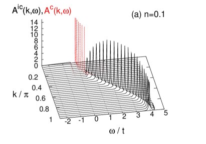
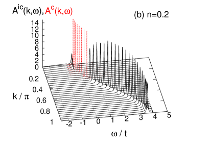
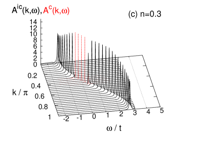
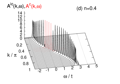
Figure 1: (colour online) Coherent ($A^{\mathrm{c}}$, -  -  -  -) and incoherent ($A^{\mathrm{ic}}$, ——) parts of the spectral function in the weak-coupling approximation for different band fillings $n$. Here $\omega_{0}/t=0.4$ and $E_{\mathrm{p}}/t=0.1$.

As in section 2.2, we first discuss the WC and SC limits, before turning to the important IC regime. Since we use a finite number of momenta $k$, it is not possible to tune the band filling $n$ (via the chemical potential $\mu$) to a specific, desired value with arbitrary accuracy. In order to simplify the discussion of the different density regimes, we therefore report rounded values of $n$ in the figures and the text. The largest deviations of the actual $n$ from the value reported occur in the SC case for which, however, the density dependence is very weak (see section 3.2).

3.1 Weak coupling

Figures 1–3 show the electronic spectral function $A(k,\omega)$ obtained from the WC approximation. The coherent spectrum ($\mathrm{Im}\,\Sigma\equiv 0$) is given as the solution of equations (10)–(2.2.1) with energies $|E_{k}-\mu|<\omega_{0}$. For $|\omega|>\omega_{0}$, $A^{\mathrm{ic}}$, calculated according to equations (13) and (14), consists of peaks having widths proportional to $E_{\mathrm{p}}$. A comparison of figures 1 (a) and 2(a) shows the spreading of the coherent spectrum with increasing $\omega_{0}$. Finally, comparing figure 1(d) [2(b)] with figure 3(a) [3(b)], we observe a broadening of the peaks in $A^{\mathrm{ic}}$ with increasing $E_{\mathrm{p}}$.

The evolution of the spectral function with increasing carrier density $n$ is illustrated in figure 1(a)–(d). The coherent part is shifted inside the spectrum as a function of $n$ (i.e., with $\mu$). Additionally, the shape of $A^{\mathrm{ic}}$ is also affected by $n$, due to the dependence of equations (13) and (14) on the chemical potential $\mu$.

In figure 4, we plot the total spectral weight $\int\rmd k\int\rmd\omega A(k,\omega)$, as well as the coherent weight $\int\rmd k\int\rmd\omega A^{\mathrm{c}}(k,\omega)$. Note that for any $E_{\mathrm{p}}>0$, the coherent band $E_{k}$ is restricted to the interval $[-\omega_{0},\omega_{0}]$, so that the corresponding coherent weight is significantly smaller than the $E_{\mathrm{p}}=0$ value of unity. This reduction is less pronounced for larger phonon frequency $\omega_{0}/t=2\approx W/t$ (figure 4). Furthermore, we see that with increasing $E_{\mathrm{p}}$, the sum rule for $A(k,\omega)$ becomes more and more violated, as expected for a WC approximation (for a more detailed discussion of sum rules see section 3.2).

Finally, figure 5 displays the coherent band dispersion $E_{k}$ at small carrier density $n=0.1$. As known from the single-polaron problem, the coherent weight $z_{k}$ drops to zero as the bare phonon dispersion intersects with the renormalized band. This gives rise to a flattening of the coherent band at large $k$ [37], which is well reproduced by the simple WC approximation.

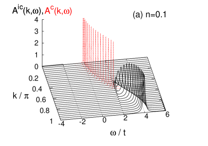
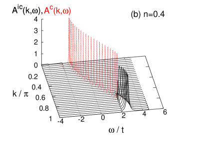
Figure 2: (colour online) As in figure 1, but for $\omega_{0}/t=2$.

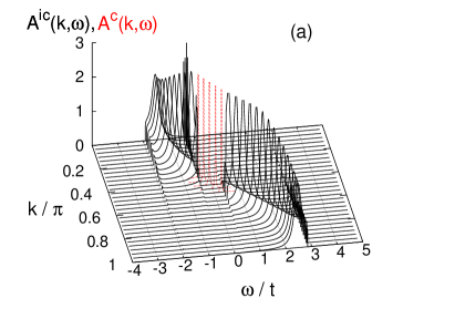
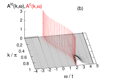
Figure 3: (colour online) As in figure 1, but for $E_{\mathrm{p}}/t=0.5$ and fixed band filling $n=0.4$. Here (a) $\omega_{0}/t=0.4$ and (b) $\omega_{0}/t=2$.

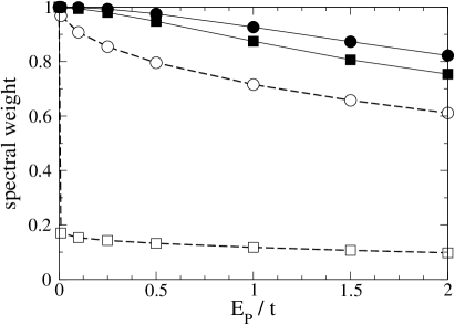
Figure 4: Coherent (-  -  -  -) and total (——) spectral weight from $A(k,\omega)$ (see text) for $\omega_{0}/t=0.4$ ($\opensquare$, $\fullsquare$) and $\omega_{0}/t=2$ ($\opencircle$, $\fullcircle$) as a function of the polaron binding energy $E_{\mathrm{p}}$. Here $\mu=0$.

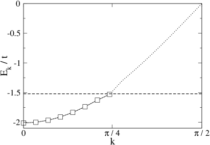
Figure 5: Renormalized band $E_{k}$ for $\omega_{0}/t=0.4$, $E_{\mathrm{p}}/t=0.1$ and $n=0.1$. Symbols indicate non-zero coherent spectral weight $z_{k}$. The horizontal line (-  -  -  -) corresponds to $(E_{0}+\omega_{0})/t$.

3.2 Strong coupling

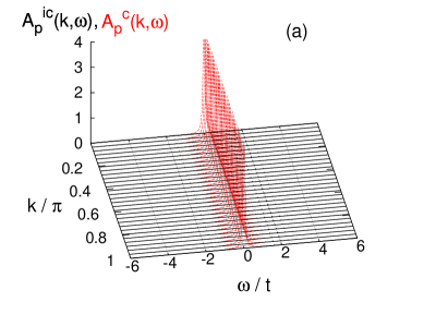
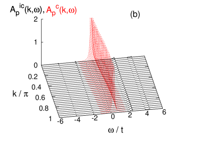
Figure 6: (colour online) Coherent ($A_{\mathrm{p}}^{\mathrm{c}}$, -  -  -  -) and incoherent ($A_{\mathrm{p}}^{\mathrm{ic}}$, ——) parts of the polaron spectral function in the strong-coupling approximation. Here $n=0.4$, $E_{\mathrm{p}}/t=4$ and (a) $\omega_{0}/t=0.4$, (b) $\omega_{0}/t=2$.

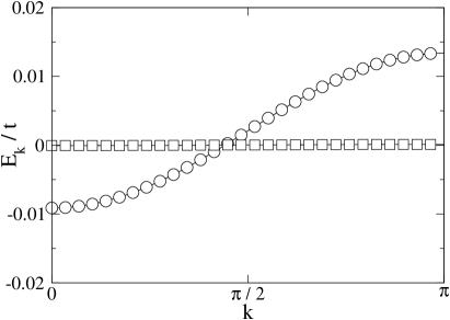
Figure 7: Renormalized band $E_{k}$ for $n=0.4$, $\omega_{0}/t=0.4$ and different values $E_{\mathrm{p}}/t=2$ ($\opencircle$) and $E_{\mathrm{p}}/t=4$ ($\opensquare$).

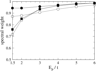
Figure 8: Coherent (polaronic, -  -  -  -) and total (——) spectral weight from $A_{\mathrm{p}}(k,\omega)$ for $\omega_{0}/t=0.4$ ($\opensquare$, $\fullsquare$) and $\omega_{0}/t=2$ ($\opencircle$, $\fullcircle$), as a function of the polaron binding energy $E_{\mathrm{p}}$. Here $\mu=0$.

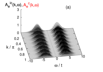
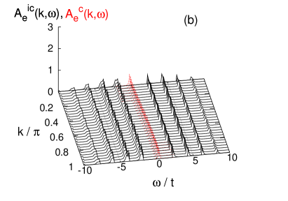
Figure 9: (colour online) As in figure 6, but showing the electronic spectral functions $A_{\mathrm{e}}^{\mathrm{c}}$ (-  -  -  -) and $A_{\mathrm{e}}^{\mathrm{ic}}$ (——).

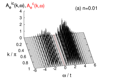
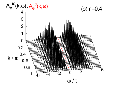
Figure 10: (colour online) As in figure 9, but for different band fillings $n$. Here $\omega_{0}/t=0.4$ and $E_{\mathrm{p}}/t=2$.

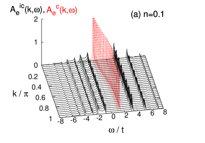
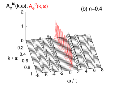
Figure 11: (colour online) As in figure 10, but for $\omega_{0}/t=2$.

We now turn to the opposite, SC limit. The theory presented in section 2.2.2 directly yields the polaronic spectrum $A_{\mathrm{p}}(k,\omega)$, results for which are shown in figure 6(a) for $\omega_{0}/t=0.4$ and $E_{\mathrm{p}}/t=4$. The spectrum is dominated by a coherent polaronic band with negligible width (for the dependence of the bandwidth on $E_{\mathrm{p}}$ see figure 7) having a spectral weight $z_{k}$ close to unity (cf. figure 8). This suggests that small polarons are the correct quasiparticles in the SC regime. Note that opposite to the WC case, where the sum rule for the spectral function becomes more and more violated with increasing coupling (figure 4), here the SC approximation becomes increasingly better with increasing $E_{\mathrm{p}}$ (figure 8).

We would like to point out that such changes in the total spectral weight are absent in the work of Alexandrov and Ranninger [34], since the latter was restricted to the lowest (first) order of the self-energy, similar to the Hartree approximation discussed in section 2.2.3. In general, the total spectral weight contained in the (electronic or polaronic) spectral function for given parameters depends on the approximations made. As illustrated by figures 4 and 8, the total spectral weight approaches the exact value of unity in the WC and SC regimes, respectively, so that the normalization of the spectrum serves as a measure of the validity of the underlying approximations. Since in the present case even the first moment (i.e., the normalization) shows deviations from exact results, we have refrained from checking the more complicated sum rules derived in [39]. This is also true of the IC case discussed below.

The effect of increasing the phonon frequency $\omega_{0}$ can be seen by comparing figures 6(a) and (b). Most noticeably, for larger $\omega_{0}$, the width of the coherent polaron band—roughly scaling proportional to $\rme^{-g^{2}}$—is larger.

The polaronic spectrum is related to the electronic spectrum $A_{\mathrm{e}}$ by equation (2.2.2), and typical results in the adiabatic and non-adiabatic regimes are shown in figure 9. Although strictly speaking a distinction between coherent and incoherent contributions cannot be made in the case of $A_{\mathrm{e}}$ [cf. equation (2.2.2)], it is useful to separate the two terms on the r. h. s. of equation (2.2.2), and to identify the first as the contribution of the coherent polaron band.

Carrying out the transformation from $A_{\mathrm{p}}$ to $A_{\mathrm{e}}$ according to equation (2.2.2), the weight of the coherent polaron band visible in figure 6 approximately acquires a prefactor $\rme^{-g^{2}}$. The remaining contributions to the electronic spectrum correspond to phonon-assisted photoemission processes.

In the case of $A_{\mathrm{e}}$, the main difference between the adiabatic [figure 9(a)] and the non-adiabatic regime [figure 9(b)] is the significantly larger weight of the coherent band for large $\omega_{0}$ since $g^{2}=E_{\mathrm{p}}/\omega_{0}$. Consequently, the weight contained in the incoherent excitations is noticeably reduced.

The results in figures 10 and 11 show a certain dependence on the band filling $n$, but there occur no qualitative changes even at IC $E_{\mathrm{p}}/t=2$. This is in contrast to recent numerical work [24, 25]. In particular, the spectrum in figure 10(b) is substantially different from figures 14(c) and (d), which are all for the same parameters. We shall see below that a more satisfactory description of the real physics can be obtained using the variational approach discussed in section 2.2.3.

3.3 Cross-over from weak to strong coupling

Figure 12: Total energy per site $E/N$ as a function of the variational parameter $R$ for different values of $E_{\mathrm{p}}$ from the Hartree approximation. Here $n=0.4$ and (a) $\omega_{0}/t=0.4$, (b) $\omega_{0}/t=2$. The values of $E_{\mathrm{p}}/t$ are (from top) (a) 0.1, 1, 2, 2.5, 3, 4, (b) 0.1, 1, 2, 4, 6, 8, and 12.

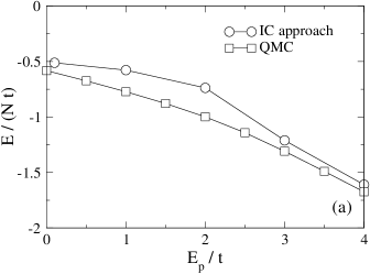
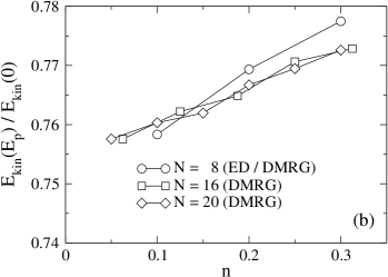
Figure 13: (a) Total energy per site $E/N$ as a function of $E_{\mathrm{p}}$ obtained from $A(k,\omega)$ (see text), where $n=0.4$ and $\omega_{0}/t=0.4$. Also shown are quantum Monte Carlo results at inverse temperature $\beta t=8$ obtained with the method of [24]. (b) Exact diagonalization (ED) and density matrix renormalization group (DMRG) results for the renormalized kinetic energy as a function of carrier density $n$ for $E_{\mathrm{p}}/t=2$, $\omega_{0}/t=0.4$ and different cluster sizes $N$.

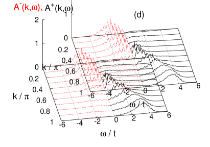
Figure 14: (colour online) Spectral functions from the variational approach for different values of $E_{\mathrm{p}}$, $n=0.4$ and $\omega_{0}/t=0.4$. The parameters are (a) $E_{\mathrm{p}}/t=0.1$, $R=1.5$, (b) $E_{\mathrm{p}}/t=4$, $R=0.1$ and (c) $E_{\mathrm{p}}/t=2$, $R=1.3$. The values of $R$ have been chosen according to figure 12(a). Panel (d) shows cluster perturbation theory results for photoemission [$A^{-}(k,\omega)$, dashed lines] and inverse photoemission [$A^{+}(k,\omega)$] for $n=0.4$ and $E_{\mathrm{p}}=2$ (taken from [25]).

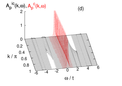
Figure 15: (colour online) Spectral functions from the variational approach for different values of $E_{\mathrm{p}}$, $n=0.4$ and $\omega_{0}/t=2$. The parameters are (a) $E_{\mathrm{p}}/t=0.1$, $R=0.7$, (b) $E_{\mathrm{p}}/t=8$, $R=0.2$, (c) and (d) $E_{\mathrm{p}}/t=4$, $R=0.5$. The values of $R$ have been chosen according to figure 12(b). In the white regions in (d) $A_{\mathrm{p}}^{\mathrm{ic}}<0$ (see text).

As seen in the preceding sections, both the WC and SC approximations are not capable of accounting for the recently discussed carrier density-driven cross-over from a polaronic system to a metallic system with phonon-dressed electrons [24, 25]. In fact, the electronic spectrum always remains WC/SC-like in character. In order to obtain a reasonable, analytical description of the IC regime, we therefore use the variational approach proposed in section 2.2.3.

Figure 12 shows results for the total energy per site as a function of the variational parameter $R$ for different values of $E_{\mathrm{p}}$. The evolution is very similar to the large-to-small polaron cross-over in the one-electron case [32]. Note that the present results have been obtained using the Hartree approximation, as discussed in section 2.2.3.

For weak coupling $E_{\mathrm{p}}$, in the adiabatic case [figure 12(a)], we find a minimum in the total energy at a finite value of $R$. Upon increasing $E_{\mathrm{p}}$, a second local minimum starts to develop near $R=0$, associated with the small-polaron state which becomes the ground state in the SC limit. The jump of the optimal value of $R$ from a large to a small value at a critical $E_{\mathrm{p}}$ suggests a first-order transition from an extended to a small-polaron state. However, such a sharp transition is absent in the single-polaron case, and not expected for $n>0$ either. The discontinuous cross-over appearing in our results for $\omega_{0}/t\lesssim 1$ is a consequence of the approximation used.

In contrast, in the non-adiabatic regime [figure 12(b)], there exists only a single minimum, which shifts to smaller $R$ with increasing coupling $E_{\mathrm{p}}$. Moreover, compared to figure 12(a), the dependence of the total energy on $R$ is much weaker.

Apart from the comparison of the spectral function with other methods presented below, variational approaches—often not capable of yielding dynamic properties—are usually judged by the total energy as opposed to exact data. Figure 13(a) shows the second-order results for the total energy as a function of $E_{\mathrm{p}}$, using the optimal values of the parameter $R$ as determined from the Hartree approximation. Clearly, the agreement between our IC approach and results from quantum Monte Carlo [24] is very good at weak and strong coupling (the variational approach reproduces the WC and SC limits of sections 2.2.1 and 2.2.2), whereas there are notable deviations at IC. The missing higher-order corrections—causing the violation of the sum rule discussed earlier—lead to generally overestimated values of the energy. Note that the agreement of the energy with exact results is even better in the non-adiabatic regime (not shown).

To illustrate the density-driven cross-over from (large) polarons to slightly dressed electrons (scattered by diffusive phonons), figure 13(b) reports exact numerical results for the renormalized kinetic energy. The latter may serve as a measure for the carrier mobility. The increase as a function of $n$ may be interpreted as originating from the overlap of the displacement clouds surrounding the carriers and, finally, the dissociation of the polaronic quasiparticles at large $n$.

We again begin the discussion of the spectral functions with the adiabatic case $\omega_{0}/t=0.4$. Following the discussion of section 2.2.3, we determine the optimal $R$ from the position of the minimum of the total energy for given $E_{\mathrm{p}}$ and $n$ (figure 12).

Figures 14(a) and (b) resemble closely to the WC and SC results of figures 1(d) and 10(b), respectively. However, for IC $E_{\mathrm{p}}/t=2$ [figure 14(c)], we find a rather metallic spectrum with a broad main band crossing the Fermi level, and with low-energy excitations available. The corresponding polaronic spectrum (not shown) reveals that the variational approach correctly predicts the absence of well-defined polaronic quasiparticles, as suggested by the non-negligible incoherent contributions in $A_{\mathrm{p}}(k,\omega)$, lying close in energy to the coherent band. This is in contrast to the SC case, where polaronic quasiparticles dominate, and in which the coherent band is well separated from the incoherent excitations. Note that in figure 14(c) [and also in figures 15(c) and (d)] the incoherent part becomes slightly negative for $\omega\gtrsim-W$ ($\omega\lesssim W$) at large (small) $k$, which is an artifact of our approximation. Remarkably, the overall features of the spectrum in figure 14(c) are very similar to the corresponding numerical results in [25], reproduced in figure 14(d).

Finally, in the non-adiabatic regime, it has been found numerically that small polarons remain the correct quasiparticles even at large band fillings $n$ [23, 24]. Again, the variational approach is able to describe the physics correctly. In particular, figures 15(c) and (d) reveal that a dominant coherent band, well separated from incoherent excitations and having a relatively small bandwidth, exists even at IC.

As for the WC and SC cases discussed above, we have also checked the total spectral weight in the present case. We find that the deviations from the exact value of unity are largest for WC, whereas the sum rule is fulfilled to within 1-10% (depending on $\omega_{0}$ and $E_{\mathrm{p}}$) at IC and SC.

4 Conclusion

We have presented an analytical treatment of the one-dimensional spinless Holstein model based on calculations of the self-energy in the framework of the generalized Matsubara functions. To connect the analytical results to previous numerical ones, the electronic spectral function determining the photoemission spectrum has been computed for finite carrier concentrations in dependence on the electron-phonon coupling strength and the phonon frequency.

In the strong-coupling limit, the electron spectral function has been deduced from the spectral function of small polarons. However, it was shown that the electron picture and the small-polaron picture both cease to be correct if we approach the intermediate-coupling regime from the weak– and strong-coupling side, respectively.

To describe the cross-over from the strong– to the weak-coupling limit, an interpolation scheme based on a generalization of the Lang-Firsov canonical transformation has been proposed. The latter was defined for each set of model parameters by a distance $R$ which characterizes the charge distribution across the polaron volume. The parameter $R$, as deduced from the minimum of the total energy in the first approximation, was shown to increase with decreasing $E_{\mathrm{p}}$—corresponding to a cross-over from large to small polarons—and, at the same time, the coupling dependence of $R$ was found to be stronger in the adiabatic than in the non-adiabatic case.

The spectral functions calculated at weak, strong and intermediate coupling are in a good agreement with recent numerical calculations. Moreover, analytical results deduced by means of the self-energy calculations enabled us to distinguish between the coherent and incoherent parts of the spectrum. Most importantly, starting from the strong-coupling limit, it was shown that the spectral weight of the incoherent polaron spectrum increases with decreasing coupling $E_{\mathrm{p}}$, and that the energy separation of the incoherent peaks from the coherent spectrum is continuously reduced in the adiabatic regime. On the contrary, the coherent part of the electronic (photoemission) spectra is reduced by a factor $\rme^{-g^{2}}$, and the incoherent part representing the phonon-assisted photoemission processes becomes increasingly dominant with increasing coupling.

Finally, at intermediate coupling and finite carrier densities, our results support recent numerical findings which suggest that the system can no longer be described in terms of (small) polaronic quasiparticles [24, 25].

References

References

- [1] A. R. Bishop and B. I. Swanson, Los Alamos Science 21 133 (1993).
- [2] I. H. Campbell and D. L. Smith, Solid State Phys. 55, 1 (2001).
- [3] A. S. Alexandrov and N. F. Mott, Polarons and Bipolarons (World Scientific, Singapore, 1995).
- [4] G. Zhao, K. Conder, H. Keller, and K. A. Müller, Nature (London) 381, 676 (1996).
- [5] D. M. Edwards, Adv. Phys. 51, 1259 (2002).
- [6] T. Holstein, Ann. Phys. (N.Y.) 8, 325 (1959).
- [7] V. Meden, K. Schönhammer, and O. Gunnarsson, Phys. Rev. B 50, 11 179 (1994).
- [8] H. Sumi, J. Phys. Soc. Jpn. 33, 327 (1972);
- [9] [] S. Ciuchi, F. de Pasquale, S. Fratini, and D. Feinberg, Phys. Rev. B 56, 4494 (1997).
- [10] J. Ranninger and U. Thibblin, Phys. Rev. B 45, 7730 (1992).
- [11] G. Wellein, H. Röder, and H. Fehske, Phys. Rev. B 53, 9666 (1996).
- [12] L.-C. Ku, S. A. Trugman, and J. Bonča, Phys. Rev. B 65, 174306 (2002).
- [13] M. Hohenadler, H. G. Evertz, and W. von der Linden, Phys. Rev. B 69, 024301 (2004);
- [14] [] M. Hohenadler, M. Aichhorn, and W. von der Linden, Phys. Rev. B 71, 014302 (2005).
- [15] P. E. Spencer, J. H. Samson, P. E. Kornilovitch, and A. S. Alexandrov, Phys. Rev. B 71, 184310 (2005).
- [16] R. J. Bursill, R. H. McKenzie, and C. J. Hamer, Phys. Rev. Lett. 80, 5607 (1998);
- [17] [] H. Fehske, M. Holicki, and A. Weiße, Adv. Sol. State Phys. 40, 235 (2000);
- [18] [] M. Capone and S. Ciuchi, Phys. Rev. Lett 91, 186405 (2003);
- [19] [] S. Sykora et al., Phys. Rev. B 71, 045112 (2005).
- [20] Q. S. Hu and H. Zheng, Eur. Phys. J. B 28, 255 (2002);
- [21] [] H. Zheng, J. Phys.: Condens. Matter 36, 9405 (2003).
- [22] S. Datta, A. Das, and S. Yarlagadda, Phys. Rev. B 71, 235118 (2005).
- [23] M. Capone, M. Grilli, and W. Stephan, Eur. Phys. J. B 11, 551 (1999).
- [24] M. Hohenadler et al., Phys. Rev. B 71, 245111 (2005).
- [25] M. Hohenadler, G. Wellein, A. Alvermann, and H. Fehske, cond-mat/0505559, Physica B (2006);
- [26] [] G. Wellein et al., cond-mat/0505664, Physica B (2006).
- [27] I. G. Lang and Y. A. Firsov, Zh. Eksp. Teor. Fiz. 43, 1843 (1962), [Sov. Phys. JETP 16, 1301 (1962)].
- [28] L. P. Kadanoff and G. Baym, Quantum Statistical Mechanics (Benjamin-Cumming, Reading, MA, 1962).
- [29] V. L. Bonch-Bruevich and S. V. Tyablikov, The Green Function Method in Statistical Mechanics (North-Holland Publ. Co., Amsterdam, 1962).
- [30] J. Schnakenberg, Z. Phys. 190, 209 (1966).
- [31] J. Loos, Z. Phys. B 96, 149 (1994).
- [32] H. Fehske, J. Loos, and G. Wellein, Z. Phys. B 104, 619 (1997); Phys. Rev. B 61, 8016 (2000).
- [33] G. D. Mahan, Many-Particle Physics, 2nd ed. (Plenum Press, New York, 1990).
- [34] A. S. Alexandrov and J. Ranninger, Phys. Rev. B 45, 13 109 (1992).
- [35] A. S. Alexandrov, Theory of superconductivity: from Weak to Strong Coupling (IoP Publishig, Bristol, 2003), pp.110-116.
- [36] H. Zheng, D. Feinberg, and M. Avignon, Phys. Rev. B 51, 11 557 (1990).
- [37] W. Stephan, Phys. Rev. B 54, 8981 (1996);
- [38] [] G. Wellein and H. Fehske, Phys. Rev. B 55, 4513 (1997).
- [39] P. E. Kornilovitch, Europhys. Lett. 59, 735 (2002).