Topological swimming in a quantum sea

Abstract

We propose a quantum theory of swimming for swimmers that are small relative to the coherence length of the medium. The quantum swimming equation is derived from known results on quantum pumps. For a one-dimensional Fermi gas at zero temperature we find that swimming is topological: The distance covered in one swimming stroke is quantized in half integer multiples of the Fermi wave length. Moreover, one can swim without dissipation.

The theory of classical swimming studies how a cyclic change in the shape of a swimmer immersed in a fluid leads to a change in its location. The theory is both elegant and practical wilczek ; childress and has been applied to the swimming and flying of organisms, robots purcel and microbots najafi ; nature .

A classical medium may be viewed as a limiting case of quantum medium when the quantum coherence length is small compared to the size of the swimmer and interference is negligible. Quantum mechanics takes over once the swimmer is small enough. Our primary goal here is to present a theory of swimming in quantum media. We concentrate on swimming in a one dimensional ideal Fermi gas at low temperatures but our methods are more general and can be applied to higher dimensions. One dimension is distinguished in that interference effects are especially strong (and also leads to tractable and soluble models).

The swimmer, a q-swimmer, is an object with internal degrees of freedom which, we assume, are slow and classical while the degrees of freedom of the medium are fast and quantum. Swimming is accomplished by the internal degrees of freedom, the controls, undergoing periodic cycles. An example of a q-swimmer might be a molecule immersed in a quantum gas. The control of the internal configuration might be either external (through the application of external fields) or internal (due to autonomous dynamics).

Natural q-swimmers and artifical q-bots may be regarded as quantum machines that propagate by pumping the quantum particles of the ambient medium. This point of view reflects an intimate connection between quantum pumps marcus and q-swimming which will play a role below.

Consider a simple model of a swimmer made of $n$ disconnected spheres of radii $a_{j}$ immersed in either a classical or quantum medium. The swimmer can control the $n-1$ relative distances $\ell_{i}=X_{i}-X_{n},\ i=1,\dots,n-1$ between the centers $X_{i}$ of the spheres and the radii $a_{j}$. Allow the swimmer to change adiabatically the control parameters $a_{j}$ and $\ell_{i}$. The notion of adiabaticity means that the velocities, e.g. $\dot{X}_{j}$, $\dot{a}_{j}$, are small compared with the characteristic velocities of the particles in the medium. By linear response, the force on the j-th sphere is given by

$$f_{j}=-\sum_{k}\eta_{jk}\dot{X}_{k}-\sum_{k}\nu_{jk}\dot{a}_{k}+\sum_{k}F_{jk}.$$ (1)

Here $F_{ji}=-F_{ij}$ are internal forces acting between $i$ and $j$ spheres and $\eta_{jk}$, $\nu_{jk}$ are coefficients, which, a-priori, depend on the state of the swimmer (i.e. the relative distances $\ell_{i}$ and the radii of the spheres $a_{j}$) and the nature of the medium.

To derive an explicit form of the swimming equation one first needs to make a choice how to designate the position of the swimmer, $X$. For a swimmer made of $n$ disconnected pieces it is convenient to pick $X=X_{n}$, the coordinate of one of the components. The total force $\sum_{j}f_{j}$ acting on an adiabatic swimmer must vanish. (This follows from the fact that the friction forces are of first order in the adiabaticity while the acceleration is second order.) This constraint determines the swimming equation

$$-\eta\,\kern-1.00006pt{\raise 3.44444pt\hbox{ -}}\kern-6.00006pt{d}X=\sum_{i=1}^{n-1}\eta_{i}\,d\ell_{i}+\sum_{j=1}^{n}\nu_{j}\,da_{j}\,,$$ (2)

where $\eta_{k}=\sum_{j=1}^{n}\eta_{jk}\,,\eta=\sum_{j=1}^{n}\eta_{j}\,,\nu_{k}=\sum_{j=1}^{n}\nu_{jk}$. Swimming is manifestly geometric being independent of the (time) parametrization of the swimming stroke. The notation $\kern-1.00006pt{\raise 3.44444pt\hbox{ -}}\kern-6.00006pt{d}X$ stresses that the position of the swimmer will, in general, not integrate to a function on the space of controls: $X$ will not return to its original values when the controls undergo a cycle.

Eq. (2) does not determine the coefficients $\eta_{i}$, $\nu_{j}$ and $\eta$. In this sense, the swimming equation, although general, is incomplete. We start by deriving a new formula for the quantum friction $\eta$ berry . $\eta$ expresses the friction acting on an idle q-swimmer while it is being dragged at small velocity through the ambient quantum medium. The formula is in the spirit of Landauer formula landauer ; imry ; It is expressed in terms of the scattering data. As usual in the Landauer setting we assume a one dimensional system. For the sake of simplicity, we focus on the two channel case.

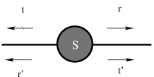
Figure 1: A scatterer with two scattering channels: $(r,t)$ and $(r^{\prime},t^{\prime})$ are the reflection and transmission amplitudes

The most general on-shell scattering matrix of a one dimensional time-reversal invariant scatterer anchored at the origin, can be parameterized as follows :

$$S_{0}\equiv\left(\begin{array}[]{cc}t&r^{\prime}\\ r&t^{\prime}\\ \end{array}\right)=e^{i\gamma}\left(\begin{array}[]{cc}i\sin\theta&e^{-i\alpha}\cos\theta\\ e^{i\alpha}\cos\theta&i\sin\theta\\ \end{array}\right).$$ (3)

The reflection $r$, $r^{\prime}$ and transmission $t$, $t^{\prime}$ amplitudes are functions of three independent real parameters: $\alpha,\gamma,\theta$.

The scattering matrix of a scatterer located at $X$ is related to the scattering matrix located at the origin, $S_{0}$, by:

$$S(X)=e^{iPX/\hbar}S_{0}e^{-iPX/\hbar},$$ (4)

where the on-shell momentum matrix $P$ is defined by

$$P=p(E)\left(\begin{array}[]{cc}1&0\\ 0&-1\\ \end{array}\right),$$ (5)

$p(E)=\sqrt{2mE}$ for electron gas and $p(E)=E/c$ for photons.

A dragged scatterer may be thought of as a pump. If the velocity of dragging is small compared with the characteristic velocity of the scattered particles, the theory of adiabatic pumps can be applied. In particular, the rate of momentum transfer to the ambient medium is ref:aegs :

$$\dot{\cal P}(t)=-\frac{1}{2\pi\hbar}\int dE\,\rho^{\prime}(E)\,Tr_{E}\,\Big{(}{\cal E}(E,t)\,P\,\Big{)},$$ (6)

${\cal E}(E,t)=i\hbar\,\dot{S}\,S^{*}$ is called the energy shift matrix martin . It depends on a frozen on-shell scattering matrix and its time derivative. Here and after $S^{*}$ denotes the Hermitian conjugate of $S$, $Tr_{E}$ denotes the trace on the scattering channels at fixed energy $E$ and $\rho(E)$ gives the occupation of the (scattering) states at energy $E$. If the ambient quantum gas is at thermal equilibrium, $\rho(E)=(e^{\beta(E-\mu)}\pm 1)^{-1}$ is the Fermi-Dirac or Bose-Einstein distribution.

In dragging a scatterer, the time dependence of $S$ comes solely from the change of position, $X$. From Eq. (4) ${\cal E}=\dot{X}[P,S]S^{*}\,$. Eq. (6) determines the force $f$ on the swimmer: $f=\dot{\cal P}$.

Define, as usual, the friction coefficient, $\eta$, by $f=-\eta\dot{X}$. Combined with Eq. (6) we get a Landauer type formula for the quantum friction

$$\eta=-\frac{1}{4\pi\hbar}\int dE\,\rho^{\prime}(E)\,Tr_{E}\,\Big{(}\,[P,S][P,S]^{*}\,\Big{)}.$$ (7)

At thermal equilibrium $\rho(E)$ is a decreasing function of the energy. This implies that $\eta$ is non-negative.

For a Fermi gas at zero temperature $\rho^{\prime}(E)=-\delta(E-E_{F})$. In the two channels case one then has $\eta_{F}=\frac{2}{\pi\hbar}\,p^{2}(E_{F})\,|r(E_{F})|^{2}$. The friction depends only on the momentum and reflection at the Fermi energy, as one expects. Transparent objects are frictionless.

To derive a q-swimming equation and fix the coefficients of Eq. (2) we make use of the elementary observation that swimming is dual to pumping. A turning screw can be used to either pump or swim. The difference lies in the setup: In a pump the external forces and torques adjust to satisfy the constraints that the position and orientation of the pump are fixed while in a swimmer the position and orientation of the swimmer adjust to satisfy the constraint that there are no external forces and torques.

Assume that no external forces are applied on a swimmer which can control its scattering matrix. The rate of momentum transfer is still given by Eq. (6). Now, however, the energy shift has two terms: ${\cal E}={\cal E}_{X}+{\cal E}_{0}$. The first ${\cal E}_{X}$ (given in Eq. (6)) arises from the swimmer’s change of location, while the second ${\cal E}_{0}=i\hbar\,\dot{S}_{0}\,S_{0}^{*}$ comes from the swimming stroke.

The total force acting on an adiabatic swimmer must vanish (to first order). This means that $\dot{\cal P}$ vanishes and the equation of motion for q-swimmers, is:

$$\eta\dot{X}\ =\frac{1}{2\pi\hbar}\,\int dE\,\rho^{\prime}(E)\,Tr_{E}\,\Big{(}{\cal E}_{0}P\Big{)}\,,$$ (8)

where $\eta$ is the friction coefficient, given in Eq. (7) and $P$ is given in Eq. (5). In the two channels case the trace on the right hand side is given by

$$Tr_{E}\big{(}{\cal E}_{0}P\big{)}=\hbar p(E)\,|r|^{2}\,{\rm Im}(\,d_{t}\log(r/r^{\prime}))\,.$$ (9)

We shall now apply the q-swimming equation, Eq. (8), to swimming in a Fermi gas at zero temperature in one dimension. This case is both simple and remarkable for, as we shall see, q-swimming turns out to be topological. A small deformation of the swimming stroke does not affect the swimming distance which is an integer multiple of the Fermi wave length. This follows immediately from Eqs. (8,9) which combine to give:

$$dX=\frac{\lambda_{F}}{8\pi}\,{\rm Im}\,\big{(}d\log(r/r^{\prime})\big{)}=\frac{\lambda_{F}}{4\pi}\,d\alpha$$ (10)

where $\lambda_{F}$ is the Fermi wave length. The fact that righthand side is an exact differential of the parameter $\alpha$ has two consequences: First, to swim one must encircle the point where the scatterer is transparent, $r=r^{\prime}=0$, and second, the distance covered in a stroke is quantized as a multiple of $\lambda_{F}/2$. The result is general and does not depend on the specifics of the swimmers.

A swimmer will normally not have direct control on parameters $\alpha$. Rather, it will control some physical parameters that will determine the scattering matrix (see examples below). Consider a swimmer with two independent controls. A stroke is a closed path in the plane of controls . Since the reflection $r$ is a complex valued function of the controls, one expects that by adjusting two controls, one can find points where $r=0$ . With each such point of transparency one can associate an (integer) index that counts how many times $r$ rotates around the origin in one cycle around the point. We call the index the vorticity. The swimming distance in a closed stroke is proportional to the vorticity enclosed by the path.

Let us now consider two examples of topological swimmers.

Pushmepullyou: Consider ‘a molecule’ made of two scatterers. The scattering matrices associated with each scatterer have $\alpha_{j}=\gamma_{j}=0$ for both scatterers and $r_{1}=\cos\theta_{1}$, $r_{2}=\cos\theta_{2}$. The two scatterers are separated by distance $\ell$, see Fig. (2). The swimmer can control $\ell$, and the ratio $r_{1}/r_{2}$. The total scattering matrix of the swimmer can then be computed by considering the multiple scattering processes between the two scatterers. A computation yields for the zeros of total reflection of $r$ the solutions of:

$$e^{2ik\ell}r_{1}-r_{2}=0.$$ (11)

It follows that the vortices occur when $r_{1}=\pm r_{2}$ and the distance $2\ell$ is an integer (half and integer) multiple of wavelengths. Since the zeros are simple the vorticities are $\pm 1$.

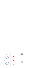
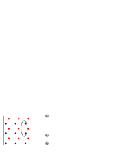
$\ell$
$r_{1}/r_{2}$      
             $\ell_{1}$
                                                    $\ell_{2}$

Figure 2: The vortex structure, at $T=0$, of Pushmepullyou (left) and the three linked spheres (right). The swimming, in both cases, is topological: The distance covered in one stroke is proportional to the sum of the vorticities encircled by the path (the ellipses in the figures). The red dots have vorticity $+1$ and the blue dots have vorticity $-1$.

Three linked spheres: Consider a swimmer (proposed by Najafi and Golestanian in najafi in a different context), made of three identical scatterers on a line, separated by distances $\ell_{1}$ and $\ell_{2}$, see Fig. 2. Take $\alpha_{j}=\gamma_{j}=0$ and $r_{j}=\cos\theta$, independent of $j=1,2,3$. The swimmer, a vibrating “trimer”, now controls only the two distances $\ell_{1},\ell_{2}$. A computation shows that the total reflection $r$ vanishes provided

$$e^{i2k\ell_{1}}+e^{-i2k\ell_{2}}-\cos^{2}\!\theta\,e^{i2k(\ell_{1}-\ell_{2})}-1=0.$$ (12)

The vortices evidently occur on a pair of lattices in the plane $(\ell_{1},\ell_{2})$, see Fig. 2. Once again, since the zeros are simple, the vorticities are $\pm 1$.

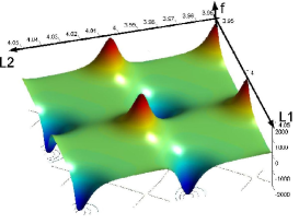
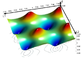
Figure 3: The curvature for the three linked spheres, shown in a 3D plot as a function of control parameters at low temperature, $T=T_{0}/4$, (above) and high temperature, $T=4T_{0}$, (below). The height of the peaks at the lower temperature is about a million times the height of the peaks at the higher temperature. The curvature vanishes as the temperature gets higher. The distance covered in one stroke is the integral of the curvature over the surface in the space of controls enclosed by the stroke.

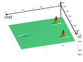
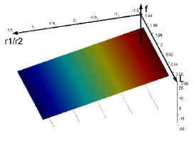
Figure 4: The curvature at finite temperatures for Pushmepullyou, shown in a 3D plot as a function of control parameters. The upper picture corresponds to the case of low temperature. The case of high temperature is shown in the lower picture. In contrasts with the three linked spheres, for Pushmepullyou the curvature does not vanish at high temperatures.

In geometrical language, Eqs. (8,10) define a connection $\kern-1.00006pt{\raise 3.44444pt\hbox{ -}}\kern-6.00006pt{d}X$ in the space of controls. The distance covered by the swimmer in a one stroke $\mathcal{C}$ is then given by $\Delta X=\int_{\mathcal{C}}\kern-1.00006pt{\raise 3.44444pt\hbox{ -}}\kern-6.00006pt{d}X$. When there are only two control parameters $(x,y)$ (as in the examples above), an application of the Stokes formula gives for the displacement $\Delta X=\int\!\!\!\int f(x,y)\,dx\,dy$, where $f(x,y)$ is the (scalar) curvature, and the domain of integration has the boundary ${\mathcal{C}}$. A plot of the curvature $f$ is often an efficient way to describe a swimmer, see e.g., Figs. 3,4.

It is instructive to see how topological Fermi swimmers are affected by temperature. At temperature $T$ a region proportional to $T$ near the Fermi energy will contribute to the integral in Eq. (8). This makes the curvature a smooth function (rather than a collection of delta functions) on the space of controls. The total curvature enclosed in a path will now depend smoothly on the path. The temperature scale is determined by $T_{0}=h^{2}/4mk_{B}\lambda_{F}\ell$ where $k_{B}$ is Boltzmann constant and $m$ the mass of the scattered particle. At this temperature the support of $f$ near a vortex becomes comparable with the distance between vortices. From the definition of $T_{0}$ it follows that the larger the swimmer (the larger $\ell$) the more sensitive it is to temperature.

Pushmepullyou and the three linked spheres have an essentially different behavior at high temperatures. Since the neighboring vortexes of three linked spheres (at $T=0$) are of opposite sign, the smearing at high temperatures leads to vanishing curvature at high temperatures, see Fig. 3. Thus the three linked spheres do not swim effectively at high temperatures. On the other hand, the smearing of the the vortices of Pushmepullyou (at $T=0$) does not lead to mutual cancellation, see Fig. 4. That means Pushmepullyou can swim effectively also at high temperatures.

In the course of its motion a swimmer will, in general, transfer energy to the medium and dissipate energy. As we shall now show, swimming without dissipation is possible in one dimensional Fermi gas at zero temperature.

We define the dissipation, $\dot{D}$, as the difference between the outgoing and incoming energy current. From ref:aegs :

$$\dot{D}=\frac{\hbar}{4\pi}Tr_{E_{F}}\big{(}\dot{S}\,\dot{S}^{*}\big{)}\geq 0.$$ (13)

One of the consequences of this relation is that a non-dissipating swimmer is indistinguishable from a static scatterer (since $\dot{S}=0$). Clearly, there is no dissipation in the former, and there should therefore be no dissipation in the latter.

To see why it is possible to swim without dissipation, write Eq. (13), (in the two channel case), in the form:

$$\dot{D}=\frac{\hbar}{2\pi}\big{(}(\dot{\alpha}-2k_{F}\dot{X})^{2}\,\cos^{2}\theta+\dot{\theta}^{2}+\dot{\gamma}^{2}\big{)}.$$ (14)

The first term vanishes by Eq. (10). Thus if $\dot{\theta}=\dot{\gamma}=0$ there is no dissipation. We call a swimming without dissipation “super-swimming”.

A super-swimmer needs a larger space of controls to ensure that $\dot{\theta}=\dot{\gamma}=0$. (For instance, to make a super-swimmer out of Pushmepullyou one needs to control also the overall phase $e^{i\gamma}$ of the two individual scatterers.) Super-swimmers are, in general, not transparent and one still needs to invest power to drag them. Only when the super-swimmer swims on its own, there is no transfer of energy to the ambient medium.

We note that no-dissipation, $\dot{S}=0$, implies Eq. (10) and hence implies quantization.

Acknowledgment This work is supported in parts by the EU grant HPRN-CT-2002-00277, the ISF, and the fund for the promotions of research at the Technion.

References

- (1) E.M. Purcell, Life at low Reynolds numbers, Am. J. Physics 45, 3-11 (1977); A. Shapere and F. Wilczek, J. Fluid Mech., 198, 557-585 (1989)
- (2) S. Childress, Mechanics of Swimming and Flying, (Cambridge University Press, Cambride, 1981); J. R. Blake, Math. Meth. Appl. Sci. 24, 1469 (2001).
- (3) L.E. Becker, S.A. Koehler, and H.A. Stone, J. Fluid Mech. 490 , 15 (2003); E.M. Purcell, Proc. Natl. Acad. Sci. 94 , 11307-11311 (1977).
- (4) A. Najafi and R. Golestanian, Phys. Rev. E69 (2004) 062901, cond-mat/0402070
- (5) R. Dreyfus, J. Baudry, M.L. Roper, M. Fermigier, H.A. Stone, J. Bibette, Nature 437, 862 - 865 (2005).
- (6) M. Switkes, C.M. Marcus, K. Campman, A.G. Gossard, Science, 283, 1907 (1999);P. W. Brouwer, Phys. Rev. B 63,121303 (2001); P.W. Brouwer, Phys. Rev. B 58, 10135 (1998).
- (7) M.V. Berry and J.M. Robbins, Proc. Roy. Soc. 422 659 (1993); D. Cohen, Phys. Rev. B 68, 155303 (2003)
- (8) R. Landauer, IBM J. Res. 1, 233 (1957); M. Büttiker, Phys. Rev. Lett. 57, 1761 (1986)
- (9) Y. Imry, Introduction to mesoscopic physics, Oxford University Press (1997).
- (10) P.A. Martin, M. Sassoli de Bianchi, J. Phys. A 28, 2403 (1995).
- (11) J. Avron, A. Elgart, G.M. Graf and L. Sadun, J. Stat. Phys. 116, 452-473 (2004)
- (12) J. Wisdom, Science 299, 1865-1869, (2003)
- (13) D. J. Thouless, Phys. Rev. B 27, 6083 (1983); Q. Niu, Phys. Rev. Lett. 64, 1812 (1990).