Slave-boson theory of the Mott transition in the two-band Hubbard model

Abstract

We apply the slave-boson approach of Kotliar and Ruckenstein to the two-band Hubbard model with an Ising like Hund’s rule coupling and bands of different widths. On the mean-field level of this approach we investigate the Mott transition and observe both separate and joint transitions of the two bands depending on the choice of the inter- and intraorbital Coulomb interaction parameters. The mean-field calculations allow for a simple physical interpretation and can confirm several aspects of previous work. Beside the case of two individually half-filled bands we also examine what happens if the original metallic bands possess fractional filling either due to finite doping or due to a crystal field which relatively shifts the atomic energy levels of the two orbitals. For appropriate values of the interaction and of the crystal field we can observe a a band insulating state and a ferromagnetic metal.

1 Introduction

The Mott transition in multiorbital systems with several bands gives rise to complex and intriguing physics. Multiband systems occur naturally in rare earth intermetallic compounds and in systems involving transition metals. In the former extended conduction electrons and almost localized $f$-electrons couple through local hybridization and give rise to Kondo and heavy Fermion physics. In transition metal oxides, chalcogenides etc. several partially filled $d$-orbitals are the origin of rather similar electron bands of different but comparable width. Here the question arises how the interaction among these orbitals, Coulomb repulsion and Hund’s rule coupling, influences the transition to partially or fully localized degrees of freedom. What is the nature of the Mott transition that occurs as the magnitude of the interactions is increased gradually? In this paper we will be concerned with these questions.

The two-band Hubbard model with bands of different widths is the simplest model that captures all the relevant aspects of the Mott transition in multiorbital systems. In recent years this model was investigated by several authors Liebsch:03 ; Liebsch:04 ; Koga:04 ; Koga:04b ; Koga:04c ; deMedici:05 ; Ferrero:05 ; Arita:05 ; Knecht:05 ; Liebsch:05 ; Inaba:05 mainly in the framework of dynamical mean-field theory (DMFT) and using different methods to solve the local impurity problem. These calculations have led to the following understanding of the Mott transition at half filling. Depending on the exact choice of the intra- and interorbital interaction parameters, one can observe a sequence of individual Mott transitions in each band or a joint transition involving both bands simultaneously. The existence of a separate transition, usually referred to as “orbital-selective Mott transition” (OSMT), implies an intermediate phase between the metal and the Mott insulator where only the narrow band is insulating whereas the wide band still has metallic properties. Furthermore, the stability of this intermediate phase strongly depends on how the Hund’s rule coupling is taken into account.

Early studies of the Mott transition in multiorbital systems made by Anisimov et al. Anisimov:02 , Liebsch Liebsch:03a ; Liebsch:03 ; Liebsch:04 ; Liebsch:05 and by Koga and coworkers Koga:04 ; Koga:04b ; Koga:04c and more recent DMFT calculations of de’ Medici et al. deMedici:05 , Ferrero et al. Ferrero:05 , Arita et al. Arita:05 , and Knecht et al. Knecht:05 showed that different impurity solvers capture different aspects of the Mott transition and can partially lead to different conclusions. It is therefore desirable to investigate the properties of this Mott transition within a more analytical theory. We apply the slave-boson approach of Kotliar and Ruckenstein KotliarRuckenstein:86 on the mean-field level, discuss and confirm several aspects of previous work. Our calculations give reasonable results in a wide range of parameters and allow in a natural way for a simple physical interpretation. Beside the case of two individually half-filled bands we examine what happens if the original metallic bands possess fractional filling either due to finite doping or due to a crystal field which shifts the atomic energy levels of the two orbitals relative to each other. In both cases we can observe an OSMT. Due to the crystal field splitting also a ferromagnetic and a band insulating phase appear in the phase diagram.

The paper is organized as follows. In Sec. 2 we introduce the model. In the rather technical Sec. 3 we apply the slave-boson formalism and its mean-field approximation. The results concerning the Mott transition are presented and discussed in Sec. 4 for various choices of the interaction parameters at half filling, in the presence of a crystal field and for finite doping. Conclusions and a comparison with previous results are found in Sec. 5.

2 Model

We consider the following two-band Hubbard Hamiltonian

$$H=\sum_{\alpha\sigma}\sum_{\langle ij\rangle}t_{ij}^{(\alpha)}c_{i\alpha\sigma}^{{\dagger}}c_{j\alpha\sigma}+\hat{V}$$ (1)

with

$$\hat{V}=U\sum_{i\alpha}\hat{n}_{i\alpha\uparrow}\hat{n}_{i\alpha\downarrow}+\sum_{i\sigma\sigma^{\prime}}(U^{\prime}-J\delta_{\sigma\sigma^{\prime}})\hat{n}_{i1\sigma}\hat{n}_{i2\sigma^{\prime}}.$$ (2)

As usual $c_{i\alpha\sigma}^{\dagger}$ ($c_{i\alpha\sigma}$) creates (annihilates) an electron with spin $\sigma=\uparrow,\downarrow$ and band index $\alpha=1,2$ at the site $i$ and $\hat{n}_{i\alpha\sigma}=c_{i\alpha\sigma}^{{\dagger}}c_{i\alpha\sigma}$ is the corresponding occupation number operator. The hopping integral for the orbital $\alpha$ is denoted by $t_{ij}^{(\alpha)}$. We assume vanishing interorbital hybridization and that the hopping integrals have different values for the different orbitals, i.e. that the tight-binding bands have different bandwidths. The intraband (interband) Coulomb repulsion is denoted by $U$ ($U^{\prime}$) and the Hund’s rule coupling by $J$. In two-band Hubbard models additional spin-flip and pair-hopping terms are usually included in the Hund’s rule coupling. As shortly discussed in the next section, these terms pose problems in the slave-boson formalism and we therefore concentrate on the Ising like Hund’s rule coupling in (2). Note however that these terms are not included in Quantum Monte Carlo (QMC) calculations either Liebsch:03 ; Liebsch:04 ; Knecht:05 . For a spherically symmetric screened Coulomb interaction the positive interaction parameters are related by $U^{\prime}=U-2J$ Castellani:78 . The relevant parameter regime is therefore $U\geq U^{\prime}$ where the intraorbital repulsion is bigger than the interorbital.

3 Slave-boson formulation of the two-band Hubbard model

3.1 Slave-boson model

The treatment of on-site interactions with slave bosons is a well established method in different fields of strongly correlated electron systems. Kotliar and Ruckenstein KotliarRuckenstein:86 introduced this approach for the (one-band) Hubbard model. By a new functional-integral representation of the partition function they were able to effectively map the fermionic action on a bosonic action with local constraints. The simplest saddle-point approximation of their approach reproduces the results of the Gutzwiller approximation BrinkmanRice:70 ; Gutzwiller:62 ; Gutzwiller:64 . The slave-boson approach leads to a novel mean-field theory which is especially useful for examining the Mott transition. As the Gutzwiller approximation, the slave-boson mean-field theory is closely related to Landau’s Fermi liquid theory Landau:56 since the slave bosons keep track of the other electrons by measuring the electron occupancy at each atom which leads to a renormalization of the hopping amplitude and thus to a change of the effective mass.

Figure 1: The sixteen atomic configurations of the two-band Hubbard model and the corresponding slave bosons.

Table 1: The atomic states in the original model, their corresponding slave-boson states as well as the labeling of the mean fields. The site index is suppressed, $\alpha=1,2$, and $\bar{\sigma}=\downarrow(\uparrow)$ if $\sigma=\uparrow(\downarrow)$.

	Original model	Slave-boson model	Mean fields
$|e\rangle$	$|0\rangle$	$e^{{\dagger}}|\mathrm{vac}\rangle$	$e\equiv\langle e^{({\dagger})}\rangle$
$|p_{\alpha\sigma}\rangle$	$c_{\alpha\sigma}^{{\dagger}}|0\rangle$	$p_{\alpha\sigma}^{{\dagger}}\hat{f}^{{\dagger}}_{\alpha\sigma}|\mathrm{vac}\rangle$	$p_{\alpha\sigma}\equiv\langle p_{\alpha\sigma}^{({\dagger})}\rangle$
$|s_{\alpha}\rangle$	$c_{\alpha\uparrow}^{{\dagger}}c_{\alpha\downarrow}^{{\dagger}}|0\rangle$	$s_{\alpha}^{{\dagger}}\hat{f}_{\alpha\uparrow}^{{\dagger}}\hat{f}_{\alpha\downarrow}^{{\dagger}}|\mathrm{vac}\rangle$	$s_{\alpha}\equiv\langle s_{\alpha}^{({\dagger})}\rangle$
$|d_{\sigma\sigma}\rangle$	$c_{1\sigma}^{{\dagger}}c_{2\sigma}^{{\dagger}}|0\rangle$	$d_{\sigma\sigma}^{{\dagger}}\hat{f}_{1\sigma}^{{\dagger}}\hat{f}_{2\sigma}^{{\dagger}}|\mathrm{vac}\rangle$	$d_{\sigma\sigma}\equiv\langle d_{\sigma\sigma}^{({\dagger})}\rangle$
$|d_{\sigma\bar{\sigma}}\rangle$	$c_{1\sigma}^{{\dagger}}c_{2\bar{\sigma}}^{{\dagger}}|0\rangle$	$d_{\sigma\bar{\sigma}}^{{\dagger}}\hat{f}_{1\sigma}^{{\dagger}}\hat{f}_{2\bar{\sigma}}^{{\dagger}}|\mathrm{vac}\rangle$	$d_{\sigma\bar{\sigma}}\equiv\langle d_{\sigma\bar{\sigma}}^{({\dagger})}\rangle$
$|h_{1\sigma}\rangle$	$c_{1\sigma}^{{\dagger}}c_{2\uparrow}^{{\dagger}}c_{2\downarrow}^{{\dagger}}|0\rangle$	$h_{1\sigma}^{{\dagger}}\hat{f}_{1\sigma}^{{\dagger}}\hat{f}_{2\uparrow}^{{\dagger}}\hat{f}_{2\downarrow}^{{\dagger}}|\mathrm{vac}\rangle$	$h_{1\sigma}\equiv\langle h_{1\sigma}^{({\dagger})}\rangle$
$|h_{2\sigma}\rangle$	$c_{1\uparrow}^{{\dagger}}c_{1\downarrow}^{{\dagger}}c_{2\sigma}^{{\dagger}}|0\rangle$	$h_{2\sigma}^{{\dagger}}\hat{f}_{1\uparrow}^{{\dagger}}\hat{f}_{1\downarrow}^{{\dagger}}\hat{f}_{2\sigma}^{{\dagger}}|\mathrm{vac}\rangle$	$h_{2\sigma}\equiv\langle h_{2\sigma}^{({\dagger})}\rangle$
$|f\rangle$	$c_{1\uparrow}^{{\dagger}}c_{1\downarrow}^{{\dagger}}c_{2\uparrow}^{{\dagger}}c_{2\downarrow}^{{\dagger}}|0\rangle$	$f^{{\dagger}}\hat{f}_{1\uparrow}^{{\dagger}}\hat{f}_{1\downarrow}^{{\dagger}}\hat{f}_{2\uparrow}^{{\dagger}}\hat{f}_{2\downarrow}^{{\dagger}}|\mathrm{vac}\rangle$	$f\equiv\langle f^{({\dagger})}\rangle$

Let us first look at one particular lattice site. The atomic Hilbert space is 16-dimensional and spanned by the local occupation number basis listed in the first column of Tab. 1 and sketched in Fig. 1. The essence of the slave-boson approach of Kotliar and Ruckenstein is to map the original fermionic model to a mixed fermionic-bosonic model with local constraints by introducing for each atomic configuration an auxiliary boson

$$\{e^{({\dagger})},p_{\alpha\sigma}^{({\dagger})},s_{\alpha}^{({\dagger})},d_{\sigma\sigma^{\prime}}^{({\dagger})},h_{\alpha\sigma}^{({\dagger})},f^{({\dagger})}\}$$ (3)

where $\alpha=1,2$, $\sigma=\uparrow,\downarrow$. The labeling of the boson operators is sketched in Fig. 1. In the following we denote the fermionic annihilation (creation) operators in the slave-boson model by $\hat{f}_{i\alpha\sigma}^{({\dagger})}$ to distinguish them from $c_{i\alpha\sigma}^{({\dagger})}$ defined in the purely fermionic model. In the extended model, the creation of a general slave-boson state is realized by acting with the bosonic creation operators (3) and the new fermionic operators on the vacuum $|\mathrm{vac}\rangle$. The states which correspond to the physical atomic states of the original model are listed in the second column of Tab. 1.

The introduction of the bosonic degrees of freedom leads to unphysical states which are eliminated by local constraints. Summing up all boson occupancy operators, we define

$$\hat{I}_{i} := e_{i}^{{\dagger}}e_{i}+\sum_{\alpha\sigma}(p_{i\alpha\sigma}^{{\dagger}}p_{i\alpha\sigma}+h_{i\alpha\sigma}^{{\dagger}}h_{i\alpha\sigma})$$ (4)

$$+\sum_{\alpha}s_{i\alpha}^{{\dagger}}s_{i\alpha}+\sum_{\sigma\sigma^{\prime}}d_{i\sigma\sigma^{\prime}}^{{\dagger}}d_{i\sigma\sigma^{\prime}}+f_{i}^{{\dagger}}f_{i}.$$

Furthermore we define the operators

$$\hat{Q}_{i1\sigma} := p_{i1\sigma}^{{\dagger}}p_{i1\sigma}+s_{i1}^{{\dagger}}s_{i1}+\sum_{\sigma^{\prime}}d_{i\sigma\sigma^{\prime}}^{{\dagger}}d_{i\sigma\sigma^{\prime}}$$ (5)

$$+h_{i1\sigma}^{{\dagger}}h_{i1\sigma}+\sum_{\sigma^{\prime}}h_{i2\sigma^{\prime}}^{{\dagger}}h_{i2\sigma^{\prime}}+f_{i}^{{\dagger}}f_{i},$$

$$\hat{Q}_{i2\sigma} := p_{i2\sigma}^{{\dagger}}p_{i2\sigma}+s_{i2}^{{\dagger}}s_{i2}+\sum_{\sigma^{\prime}}d_{i\sigma^{\prime}\sigma}^{{\dagger}}d_{i\sigma^{\prime}\sigma}$$ (6)

$$+h_{i2\sigma}^{{\dagger}}h_{i2\sigma}+\sum_{\sigma^{\prime}}h_{i1\sigma^{\prime}}^{{\dagger}}h_{i1\sigma^{\prime}}+f_{i}^{{\dagger}}f_{i}.$$

The physical subspace is given by the local constraints

$$\hat{I}_{i}-1 \equiv 0,$$ (7)

$$\hat{f}_{i\alpha\sigma}^{{\dagger}}\hat{f}_{i\alpha\sigma}-\hat{Q}_{i\alpha\sigma} \equiv 0.$$ (8)

These constraints ensure that the slave-boson states listed in the second column of Tab. 1 form a complete set in the physical local Hilbertspace of the slave-boson model. The first relation (7) represents the completeness of the boson operators, i.e., the sixteen states with one boson form a complete set in the local physical Hilbertspace of the bosons. The operators $\hat{Q}_{i\alpha\sigma}$ count the number of bosons that correspond to local configurations having an electron with spin $\sigma$ in the orbital $\alpha$. Therefore, we have to ensure with the constraint (8) that in the physical subspace the operators $\hat{Q}_{i\alpha\sigma}$ are identical to the operators $\hat{f}_{i\alpha\sigma}^{{\dagger}}\hat{f}_{i\alpha\sigma}$.

Using these constraints, the interaction term becomes quadratic in the boson operators

$$\hat{V}^{\mathrm{sb}} = \sum_{i}\Big{\{}U\sum_{\alpha}s_{i\alpha}^{{\dagger}}s_{i\alpha}+(U+2U^{\prime}-J)\sum_{\alpha\sigma}h_{i\alpha\sigma}^{{\dagger}}h_{i\alpha\sigma}$$ (9)

$$+(U^{\prime}-J)\sum_{\sigma}d_{i\sigma\sigma}^{{\dagger}}d_{i\sigma\sigma}+U^{\prime}\sum_{\sigma}d_{i\sigma\bar{\sigma}}^{{\dagger}}d_{i\sigma\bar{\sigma}}$$

$$+2(U+2U^{\prime}-J)f_{i}^{{\dagger}}f_{i}\Big{\}}.$$

The attempt to include the spin-flip and pair-hopping term in a similar way fails due to quartic fermion terms in $V^{\mathrm{sb}}$ or in the constraints. In this case additional approximations are required deMedici:05 . Whereas the interaction term has become much simpler the new formulation of our model implies that the destruction or creation of a physical fermion has to be accompanied by slave bosons,

$$c_{i\alpha\sigma} \rightarrow \tilde{z}_{i\alpha\sigma}\hat{f}_{i\alpha\sigma},$$

$$c_{i\alpha\sigma}^{{\dagger}} \rightarrow \hat{f}_{i\alpha\sigma}^{{\dagger}}\tilde{z}_{i\alpha\sigma}^{{\dagger}},$$

where

$$\tilde{z}_{i\alpha\sigma} = (1-\hat{Q}_{i\alpha\sigma})^{-1/2}z_{i\alpha\sigma}\hat{Q}_{i\alpha\sigma}^{-1/2},$$ (10)

$$z_{i1\sigma} = e_{i}^{{\dagger}}p_{i1\sigma}+p_{i1\bar{\sigma}}^{{\dagger}}s_{i1}+p_{i2\sigma}^{{\dagger}}d_{i\sigma\sigma}+p_{i2\bar{\sigma}}^{{\dagger}}d_{i\sigma\bar{\sigma}}$$

$$+s_{i2}^{{\dagger}}h_{i1\sigma}+d_{i\bar{\sigma}\sigma}^{{\dagger}}h_{i2\sigma}+d_{i\bar{\sigma}\bar{\sigma}}^{{\dagger}}h_{i2\bar{\sigma}}+h_{i1\bar{\sigma}}^{{\dagger}}f_{i},$$

$$z_{i2\sigma} = e_{i}^{{\dagger}}p_{i2\sigma}+p_{i2\bar{\sigma}}^{{\dagger}}s_{i2}+p_{i1\sigma}^{{\dagger}}d_{i\sigma\sigma}+p_{i1\bar{\sigma}}^{{\dagger}}d_{i\bar{\sigma}\sigma}$$

$$+s_{i1}^{{\dagger}}h_{i2\sigma}+d_{i\sigma\bar{\sigma}}^{{\dagger}}h_{i1\sigma}+d_{i\bar{\sigma}\bar{\sigma}}^{{\dagger}}h_{i1\bar{\sigma}}+h_{i2\bar{\sigma}}^{{\dagger}}f_{i}.$$

The “$z$-operators” keep track of the environment (bosons) during hopping processes KotliarRuckenstein:86 . The choice of the “$z$-operators” is not unique. In fact, as long as the constraints are fulfilled exactly, the “$z$-operators” can be modified by any operator which is the identity operator when restricted to the physical subspace KotliarRuckenstein:86 ; Dietrich:94 . However, the mean-field results depend on the choice of these operators. The choice of Kotliar and Ruckenstein, that we take here (10), reproduces correctly the noninteracting case in the mean-field approximation KotliarRuckenstein:86 . The slave-boson Hamiltonian is then given by

$$H^{\mathrm{sb}}=\sum_{ij\alpha\sigma}t_{ij}^{(\alpha)}\hat{f}_{i\alpha\sigma}^{{\dagger}}\tilde{z}_{i\alpha\sigma}^{{\dagger}}\tilde{z}_{j\alpha\sigma}\hat{f}_{j\alpha\sigma}+\hat{V}^{\mathrm{sb}}$$ (11)

and is fully equivalent to the original Hamiltonian provided the local constraints (7, 8) are handled exactly. They can be imposed by site dependent Lagrange multipliers $\lambda_{i}^{I}$ and $\lambda_{i\alpha\sigma}^{Q}$.

3.2 Mean-field approximation

The simplest saddle-point approximation of the grand canonical partition function $\mathcal{Z}=\mathrm{Tr}[e^{-\beta(H^{\mathrm{sb}}-\mu N^{\mathrm{sb}})}\mathcal{P}]$ is equivalent to a mean-field approximation where the Bose fields and Lagrange multipliers are treated as static and homogeneous fields. Thus, this approximation consists essentially in replacing the creation and annihilation operators of the slave bosons by site independent c-numbers which can be chosen to be real. The mean fields are listed in the fourth column of Tab. 1. In this approximation, the constraints are fulfilled only on average and the square of the mean fields can be interpreted as the probability of finding the corresponding local configuration at a particular site. The mean-field Hamiltonian with included averaged constraints can be diagonalized and yields at $T=0$ the variational ground-state energy (per site)

$$\tilde{E}_{\mathrm{G}}=\sum_{\alpha\sigma}q_{\alpha\sigma}\bar{\varepsilon}_{\alpha\sigma}+V_{MF}+\lambda_{\alpha}^{I}(I-1)-\sum_{\alpha\sigma}\lambda_{\alpha\sigma}^{Q}(Q_{\alpha\sigma}-n_{\alpha\sigma}).$$ (12)

By introducing the effective chemical potential $\mu_{\alpha\sigma}=\mu-\lambda_{\alpha\sigma}^{Q}$ in band $\alpha$ for fermions with spin $\sigma$, the average kinetic energy per site and band reads

$$\bar{\varepsilon}_{\alpha}=\bar{\varepsilon}_{\alpha\uparrow}+\bar{\varepsilon}_{\alpha\downarrow}=\sum_{\sigma}\int_{-\infty}^{\mu_{\alpha\sigma}/q_{\alpha\sigma}}d\varepsilon\varepsilon\rho_{\alpha}(\varepsilon).$$ (13)

Similarly, the density in band $\alpha$ is

$$n_{\alpha}=n_{\alpha\uparrow}+n_{\alpha\downarrow}=\sum_{\sigma}\int_{-\infty}^{\mu_{\alpha\sigma}/q_{\alpha\sigma}}d\varepsilon\rho_{\alpha}(\varepsilon).$$ (14)

The chemical potential $\mu_{\alpha\sigma}$ has to be determined from Eq. (14) for a given density. If both bands are half-filled separately one finds for example $\mu_{\alpha\sigma}=0$. The bare density of state (DOS) per spin in the band $\alpha$ is denoted by $\rho_{\alpha}$ and the mean-field Coulomb energy per site is

$$V_{\mathrm{MF}} = U\left(\sum_{\alpha}(s_{\alpha}^{2}+\sum_{\sigma}h_{\alpha\sigma}^{2})+2f^{2}\right)$$ (15)

$$+U^{\prime}\left(\sum_{\sigma\sigma^{\prime}}d_{\sigma\sigma^{\prime}}^{2}+2\sum_{\alpha\sigma}h_{\alpha\sigma}^{2}+4f^{2}\right)$$

$$-J\left(\sum_{\sigma}(d_{\sigma\sigma}^{2}+h_{1\sigma}^{2}+h_{2\sigma}^{2})+2f^{2}\right).$$

The band-renormalization factor $q_{\alpha\sigma}=\tilde{z}_{\alpha\sigma}^{2}$ can be related to the effective mass of quasiparticles of Landau’s Fermi liquid theory. For quasiparticles in the band $\alpha$ with spin $\sigma$ we have $q_{\alpha\sigma}^{-1}=m_{\alpha\sigma}^{*}/m$ BrinkmanRice:70 ; Vollhardt:84 . The vanishing of $q_{\alpha\sigma}$ therefore indicates the transition to a localized state. The mean fields and the Lagrange multipliers are determined by the stationary point of $\tilde{E}_{\mathrm{G}}$ which is a saddle point but not a minimum. With the help of the averaged constraints and of Eq. (14) we reduce the number of independent variables. The stationary point of the variational ground-state energy per site

$$E_{\mathrm{G}}=\sum_{\alpha\sigma}q_{\alpha\sigma}\bar{\varepsilon}_{\alpha\sigma}+V_{\mathrm{MF}}$$ (16)

then becomes a true minimum and can be found numerically in a rather simple way.

4 Mott transition in the two-band model within slave-boson theory

In this section we present the results concerning the Mott transition obtained by numerically minimizing Eq. (16). Unless otherwise stated we always assume a paramagnetic ground state, i.e. $n_{\alpha\uparrow}=n_{\alpha\downarrow}$, and a particle-hole symmetric bare DOS. Consequently, the following conditions are satisfied: $e=f$, $p_{\alpha}\equiv p_{\alpha\sigma}=h_{\alpha\sigma^{\prime}}$, $s\equiv s_{1}=s_{2}$, $d_{0}\equiv d_{\uparrow\downarrow}=d_{\downarrow\uparrow}$ and $d_{1}\equiv d_{\uparrow\uparrow}=d_{\downarrow\downarrow}$. This greatly reduces the computational effort.

If both bands are separately half-filled, the results of the mean-field calculations do not depend on the exact choice of the bare DOS, as long as it is particle-hole symmetric. Away from half filling, the mean-field results slightly depend on the exact choice. For simplicity, we choose throughout this section for both bands a rectangular DOS and denote its half-width by $D_{\alpha}$. The narrow band is always referred to as band 1 and the wider as band 2. Unless otherwise stated we choose the ratio of the bandwidths such that $D_{1}/D_{2}=1/2$. Energy is measured in units of the bandwidth of band 2, i.e. $2D_{2}=1$. We restrict to the relevant parameter regime $U\geq U^{\prime}$, where the intraorbital repulsion is bigger than the interorbital. In Sec. 4.1 we discuss the $U$-$U^{\prime}$ phase diagram for $J=0$ at half filling. In Sec. 4.2 we focus on the dependence of the Mott transition on the ratio $D_{1}/D_{2}$ for vanishing Hund’s rule coupling and $U=U^{\prime}$. In Sec. 4.3 we impose the condition $U^{\prime}=U-2J$. In this case we also examine the effect of a crystal field and the influence of finite doping.

4.1 $\bf{U\geq U^{\prime}}$ and $\bf{J=0}$

The phase diagram at half filling is displayed in Fig. 2. We can distinguish three different phases: a metallic state (PM), a Mott-insulating state (MI) and an intermediate state (OSMI) induced by the OSMT where the localized band 1 coexists with the metallic band 2.

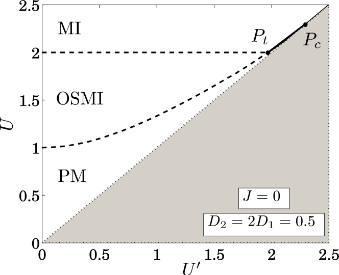
Figure 2: Phase diagram at half filling for $U\geq U^{\prime}$, $J=0$ and $D_{1}/D_{2}=1/2$. Three different phases can be distinguished: a paramagnetic metal (PM), a Mott insulator (MI) and in between an orbital selective Mott insulator (OSMI). Two second order lines (dashed) merge at $P_{t}$ to a single first order line (solid) which ends in a critical second order point $P_{c}$.

For vanishing Hund’s rule coupling, our calculations suggest that the OSMI phase is bounded by two second order lines (dashed lines in Fig. 2). They merge to a single first order line at $P_{t}$ which ends in a critical point $P_{c}$. The occurrence of this orbital selective Mott insulator is not surprising since we have neglected local spin-spin interactions. Therefore, if the first band is in a Mott-insulating state, the electrons in the second band only feel a uniform charge background (arising from the localized electrons in orbital 1) and the Mott transition in the broader band occurs at the critical interaction strength $U_{c2}=8|\bar{\varepsilon}_{2}^{o}|=4D_{2}=2$ which is the value of one independent band with bandwidth $2D_{2}=1$ KotliarRuckenstein:86 ; BrinkmanRice:70 . To understand the behavior of the system for general values $0\leq U^{\prime}\leq U$ it is instructive to consider first the following two limiting cases:

i) $U^{\prime}=0$. In this case the two bands are independent and the critical interaction strength of the Mott transition is proportional to the bandwidth $D_{\alpha}$. In Fig. 3(a) we have plotted the mean fields of the slave bosons and the band-renormalization factors. In the noninteracting system, $U=0$, all configurations are equal likely: $e=s=p_{1}=p_{2}=d=1/4$ where $d\equiv d_{0}=d_{1}$. The vanishing of $q_{1}$ is accompanied by the vanishing of $e$, $s$ and $p_{2}$, whereas $q_{2}$ becomes simultaneously zero with $p_{1}$. In the Mott-insulating phase ($U>U_{c2}$) we find at each lattice site one of the possible four atomic configurations represented by the boson $d$ and therefore $d$ reaches $1/2$ at $U=U_{c2}$.

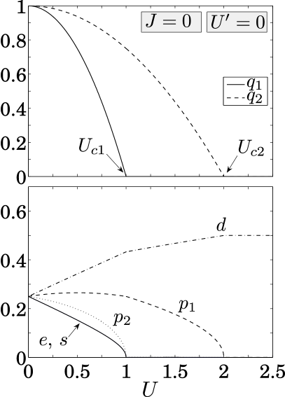
(a)

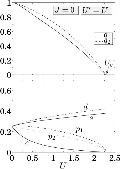
(b)

Figure 3: Mean fields of the slave bosons and band-renormalization factors $q_{\alpha}$ (a) for $U^{\prime}=J=0$ and (b) for $U=U^{\prime}$, $J=0$.

ii) $U=U^{\prime}$. For this choice the interaction Hamiltonian has an enlarged symmetry with six degenerate two-electron configurations shown in Fig. 4: four spin configurations with one electron in each orbital (represented by $d$) and two configurations with both electrons in one of the two orbitals (represented by $s$).

Figure 4: For $U=U^{\prime}$ and $J=0$ there are six degenerate two-electron on-site configurations. They are represented by the mean fields $d$ and $s$

This higher symmetry is due to the fact that the Coulomb energy of a local configuration depends only on the total charge on the atom. The additional symmetry in orbital and spin degrees of freedom enlarges the phase space for charge fluctuations and leads to a stabilization of the metallic phase Koga:04 . In Fig. 3(b) the mean fields of the slave bosons as well as the band-renormalization factors are plotted as a function of $U$. There is a joint Mott transition at the critical interaction strength $U_{c}$. Because of orbital fluctuations and in contrast to the case $U^{\prime}<U$ not only configurations represented by $d$ but also configurations represented by $s$ have a finite probability at $U_{c}$. Despite the high symmetry, it surprisingly turns out that $d\neq s$. The relative strength of the mean fields in Fig. 3(b) can be understood as follows. The high Coulomb energy of a fully occupied local configuration disfavors most strongly the mean field $e$. The effect of the intraband Coulomb interaction is stronger in the narrow band and therefore $p_{1}\geq p_{2}$ since $p_{1}$ favors localized behavior in the band 1 and itinerant behavior in the band 2. Furthermore, the $z$-factors can be approximated by $z_{1}\approx 2p_{1}s+4p_{2}d$ and $z_{2}\approx 2p_{2}s+4p_{1}d$ for high values of $U$. In order to optimize the hopping in the wide band, $d$ is slightly increased compared to $s$. Note that above $U_{c}$ the ratio of $d$ and $s$ is not determined at zero temperature.

The behavior of the system for general values $0<U^{\prime}<U$ is mostly determined by the physics of the above discussed two special choices of parameters.

4.2 $\bf{D_{1}\ll D_{2}}$, $\bf{U=U^{\prime}}$ and $\bf{J=0}$

Within our mean-field calculation the existence of a joint transition for $U=U^{\prime}$ and $J=0$ depends on the ratio of the bandwidths $D_{1}/D_{2}$. It turns out that for ratios below a critical value $(D_{1}/D_{2})_{c}$ the mean-field calculations suggest an OSMT even for $U=U^{\prime}$. Thus, we recover exactly the same results as Ferrero et al. Ferrero:05 using the Gutzwiller approximation and de’ Medici et al. deMedici:05 within their slave-spin approximation. The critical ratio where an OSMI occurs can be calculated analytically within the Gutzwiller (or slave-boson) approximation and is Ferrero:05 $(D_{1}/D_{2})_{c}=1/5$. At first sight, the existence of such a critical ratio seems to be in contradiction with the symmetry argument given by Koga et al. Koga:04 . It states that for vanishing $J$ and $U^{\prime}=U$ the Mott-Hubbard gap in both bands closes at the same critical interaction strength, independent of $D_{1}/D_{2}$. However, it does not exclude the transition into an intermediate phase, where the “localized” band is not fully gapped deMedici:05 . Indeed, DMFT calculations for $D_{1}\ll D_{2}$ Ferrero:05 ; deMedici:05 show clearly that the “localized” band is not fully gapped but has spectral weight down to arbitrarily low energies. This subtle aspect is not captured by the Gutzwiller approximation and related mean-field theories.

There is however the possibility that the OSMI phase is replaced by an instability not considered so far. Our mean-field calculation as well as earlier DMFT calculations did not take into account a possible enlargement of the unit cell. Below a critical temperature $T_{N}$ one usually finds antiferromagnetic long-range order in the Mott insulating phase depending on the topology of the lattice. Interestingly for $U^{\prime}=U$ and $J=0$ spin and orbital degrees are relevant and it is possible that the OSMI phase is unstable against an orbitally ordered phase. Whereas for $U^{\prime}<U$ there is no tendency toward such an instability it cannot be excluded a priori for $U^{\prime}=U$. We discuss now the mechanism which may drive orbital order as an another way to double the unit cell.

Let us look at the extreme limit $D_{1}\ll U=U^{\prime}\ll D_{2}$ and assume that the lattice is bipartite. In an adiabatic approximation the narrow band is localized and fully dominated by the intraorbital Coulomb repulsion ($D_{1}/U\approx 0$) whereas the intraorbital Coulomb interaction in the wide band has negligible effect ($U/D_{2}\approx 0$). We look at the following two limiting cases for the static configuration of the localized (narrow) band and their implications to the electronic properties of the wide band:

• Homogeneous charge distribution with exactly one electron per orbital.

• Staggered charge distribution with doubly occupied orbitals on one sublattice and empty orbitals on the other sublattice.

In the case (a), the homogeneous charge background contributes an amount $U$ per site to the total energy. In the case (b), the doubling of the unit cell and the induced rearrangement of electrons in the wide band opens a gap. In this way the interorbital interaction is reduced ($<U$). For perfect nesting the wide band is fully gapped and shows insulating behavior. On the other hand, the doubly occupied orbitals in the localized phase cost a fixed amount $U/2$ per site. Thus, there is a competition between these two effects which can favor an orbitally ordered phase in a certain parameter range.

In summary, the Mott transition for $U^{\prime}=U$ is a subtle issue due to the aspect of possible orbital order and we suggest that this plays a relevant role for the case $D_{1}\ll D_{2}$. Analogous to the spin ordering in the Mott insulator, the stability of such a phase depends also on details of the band structures. Taking into account the possibility of a doubling of the unit cell is an interesting topic for further investigations to be reported elsewhere.

4.3 $\bf{U\geq U^{\prime}}$ and $\bf{U^{\prime}=U-2J}$

We turn back to a given ratio $D_{1}/D_{2}=1/2$. From now on we adopt the relation $U=U^{\prime}+2UJ$ which is usually used in the discussion of the Mott transition in the two-band Hubbard model. This relation is valid for a rotationally symmetric (screened) Coulomb interaction.

4.3.1 Mott transition at half filling

The phase diagram is shown in Fig. 5. Again we can observe the OSMI phase, but it is limited to a tiny parameter regime. In general the Mott transition is shifted to smaller values of $U$ since the Ising like Hund’s rule coupling favors localized configurations with parallel spins. For the same reason the Mott transition in the second band is closer to the one in the first band because, in contrast to the case $J=0$ discussed in Sec. 4.1, the electrons in the second band not only feel a uniform charge background but also a localized spin at each lattice site after the gap for charge excitations in the first band has opened. For small values of $J$ the physics for $U^{\prime}=U$ becomes important.

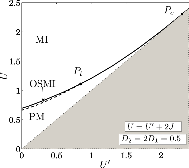
Figure 5: Phase diagram at half filling for $U=U^{\prime}+2J$ and $D_{1}/D_{2}=1/2$. Three different phases can be distinguished: a paramagnetic metal (PM), a Mott insulator (MI) and in between an orbital selective Mott insulator (OSMI). At $P_{t}$ the second order line (dashed) meets the first order line (solid) which ends in a continuous critical point $P_{c}$.

The dashed line in Fig. 5, which separates PM-OSMI, is a second order line whereas the solid line, which separates OSMI-MI and PM-MI, is a first order line. They merge at $P_{t}$. The first order line ends in a second order transition point $P_{c}$ (Fig. 3(b)).

To illustrate the occurrence of the OSMI and the first order transition line we show in Fig. 6 the slave-boson mean fields and the band-renormalization factors for a fixed ratio $U^{\prime}/U=1/2$ and $J/U=1/4$. We clearly see that there is a sequence of individual transitions and that $q_{2}$ jumps at $U\approx 0.89$ from a finite value to zero. The discontinuity is also observed in the mean fields $d_{0}$, $d_{1}$ and $p_{1}$. We computed the ground-state energy as a function of $p_{1}$ for different values of $U$, where $U^{\prime}$ and $J$ have the same ratio as above. This is shown in Fig. 7. Note that $p_{1}^{2}$ represents the probability to find at a particular site one electron in orbital 1 and either no electron or two electrons in orbital 2 and serves therefore as the order parameter for the Mott transition in the second band. At $U\approx 0.89$ the metallic solution $p_{1}\approx 0.2$ and the Mott-insulator solution $p_{1}=0$ are degenerate. This results in a first order transition and a finite jump in $p_{1}$ and consequently also in $q_{2}$ (Fig. 6).

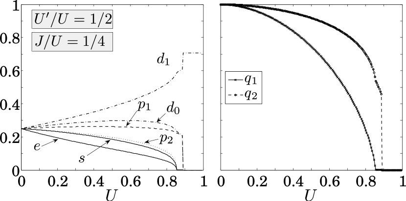
Figure 6: Mean fields of the slave bosons and band-renormalization factors $q_{\alpha}$ for $U^{\prime}/U=1/2$ and $J/U=1/4$.

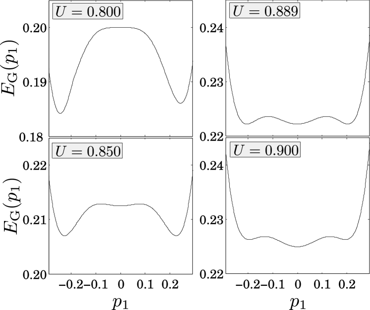
Figure 7: Ground-state energy as a function of $p_{1}$ for different values of $U$, where $U^{\prime}/U=1/2$ and $J/U=1/4$. $p_{1}$ is the order parameter for the Mott transition in the second band. At $U\approx 0.89$ the metallic solution $p_{1}\approx 0.2$ and the insulating solution $p_{1}=0$ are degenerate. This results in a first order transition.

4.3.2 Effect of a crystal field

Until now we have assumed that the two bands are both centered symmetrically around the Fermi energy. What happens if a crystal field splits the atomic energy level for the two different orbitals? Let us assume that the overall system is still half-filled. We introduce an external field $\eta\sum_{i}(\hat{n}_{i1}-\hat{n}_{i2})$ in the Hamilton operator (1) which splits the atomic energy levels by $2\eta$. Particle-hole symmetry allows to concentrate on $\eta\geq 0$. In the noninteracting case, this leads to a relative shift of the tight-binding bands by $2\eta$ and if this shift is bigger than $D_{1}+D_{2}$ the lower band is totally filled whereas the upper band is empty. In this case the system is a band insulator. How does this band insulator evolve when we turn on the Coulomb interaction? Is there a transition from the band insulator to the Mott insulator, or can we observe a new phase in between?

To answer these questions we investigate the effect of the crystal field on the mean-field level of the slave-boson approach. In contrast to the case $\eta=0$ we also keep the spin dependence of the mean fields so as to detect a possible ferromagnetically ordered state. The external field leads to an additional term in the variational ground-state energy (16), $E_{\mathrm{G}}\rightarrow E_{\mathrm{G}}+\eta(n_{1}-n_{2})$.

Let us first discuss the phase diagram for a finite Hund’s rule coupling. To be specific we fix $U^{\prime}/U=1/2$ and $J/U=1/4$. The result of the minimization of the ground-state energy for different values of $U$ and $\eta$ is shown in Fig. 8.

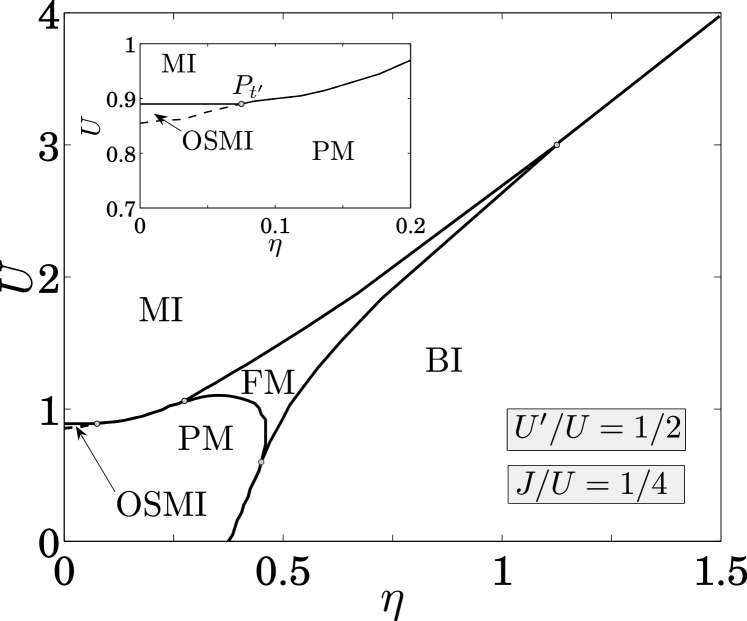
Figure 8: Phase diagram in the presence of an external field $\eta$ for $U^{\prime}/U=1/2$ and $J/U=1/4$. The OSMI is limited to a small parameter regime as shown in the inset. The crystal field introduces two new phases: a band insulator (BI) and a ferromagnetic metal (FM).

In our slave-boson approach the OSMI phase is restricted to a tiny parameter regime and only present for small values of $\eta$ as shown in the inset of Fig. 8. The transition in the first band (dashed) is a second order line which merges the first order transition line (solid) at $P_{t^{\prime}}$. If the crystal field is strong enough, the system is in a band insulating state (BI), i.e. one energy band is totally filled whereas the other is empty. For $\eta>0$ this state is characterized by the mean field $s_{2}=1$. For $U=0$ the transition PM-BI is second-order and happens at $\eta=(D_{1}+D_{2})/2=0.375$. For a finite $U$ the transition is first-order since the charge abruptly jumps from $n_{2}<1$ to $n_{2}=1$. For very strong values of $U$ and $\eta$ there is a competition between the BI and the MI phase. The boundary is given by comparing the energy of the BI phase, $U-2\eta$, with the energy $U^{\prime}-J$ of the MI phase and yields $U=8\eta/3$ for the above given ratio of the interaction parameters. The most interesting region of Fig. 8 lies between these limiting cases where a ferromagnetically ordered metal (FM) is observed. This state is twofold degenerated and triggered by the finite Hund’s rule coupling. Within our approximation we always find maximal spin polarization which is characterized by a finite value of the mean fields $\{s_{2},h_{1\sigma},d_{\sigma\sigma},p_{2\sigma}\}$. We can get an idea of the physical mechanism by fixing $\eta=0.5$ and increasing $U$ continuously starting at $U=0$. The evolution of the charge is shown in Fig. 9.

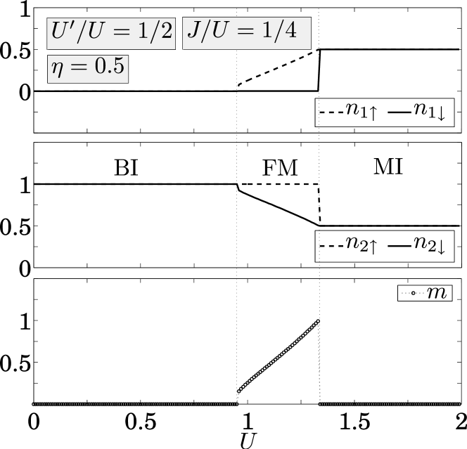
Figure 9: The evolution of the charges in the two bands for $U^{\prime}/U=1/2$ and $J/U=1/4$ and the magnetization $m=n_{\uparrow}-n_{\downarrow}$ for fixed $\eta=0.5$.

At the beginning the Coulomb repulsion is too weak to put electrons in the upper band and $n_{2\uparrow}=n_{2\downarrow}=1$. At a critical interaction strength it is energetically favorable to populate the upper band by a few electrons of the same spin species and $n_{1\uparrow}$ jumps from $0$ to a finite value. In the lower band $n_{2\downarrow}$ simultaneously jumps from $1$ to a value $n_{2\downarrow}<1$. The Pauli principle excludes doubly occupied orbitals in the upper band which reduces the Coulomb energy and leads to a ferromagnetic order. In addition, $J$ couples the spin between upper and lower band and we find the same magnetization in both bands: $m_{1}=m_{2}=m/2$. Note that the critical interaction for the transition to the FM phase depends on the exact choice of the bare DOS. Increasing $U$ further increases $n_{1\uparrow}$ up to 1/2 where we find a first-order transition from the ferromagnetic metal to the Mott insulator.

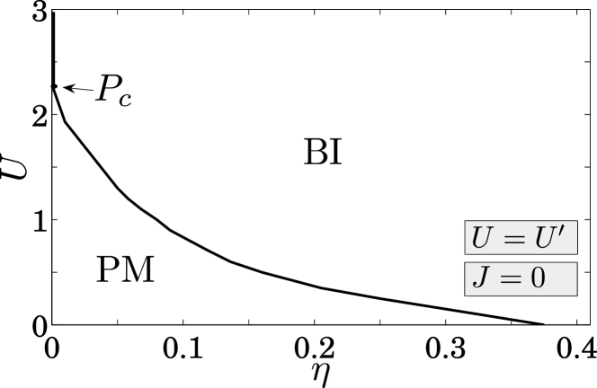
Figure 10: Phase diagram in the presence of an external field $\eta$ for $U=U^{\prime}$ and $J=0$. At the breakdown of the metallic solution (PM) there is a transition to a band insulating phase (BI).

Let us now turn to the case of vanishing Hund’s rule coupling $J=0$ and $U^{\prime}=U$. As shown in Fig. 10, a qualitatively different phase diagram is observed. For $\eta=0$ we saw in Sec. 4.1 that the paramagnetic metal is quite stable due to the enhanced degeneracy of the lowest atomic configurations and that there is a joint transition to the Mott-insulating phase. This continuous transition is denoted by $P_{c}$ in Fig. 10. An arbitrarily small field $\eta$ lowers the energy of the BI phase compared to the Mott insulator and therefore we find at the breakdown of the metallic solution for any finite $\eta$ and $U$ a first-order transition to the BI phase characterized by the mean field $s_{2}=1$. Similar to a finite $J$, a finite $\eta$ lifts the degeneracy of the six lowest on-site configurations, orbital fluctuations are suppressed and therefore the stability of the metallic phase is reduced with increasing crystal field.

Note that our calculations simplify the true behavior of the system near the transition lines because the uniform mean-field approximation always reproduces the results of the atomic limit whenever the kinetic energy vanishes. Nevertheless they give some insight of the rich behavior of the system in the present of a crystal field which relatively shifts the atomic energy levels of the two orbitals.

4.3.3 Mott transition away from half filling

We now address the question of what happens away from half filling, $n=2-2\delta$, but again with zero crystal-field splitting. Particle-hole symmetry allows to concentrate on $\delta>0$. In general we observe a Mott transition in the narrow band which lies at an increased interaction strength compared to the case $\delta=0$ (see Fig. 11).

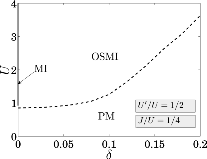
Figure 11: Dependence of the Mott transition on the level of doping.

Because the second band is always away from half filling it stays metallic.

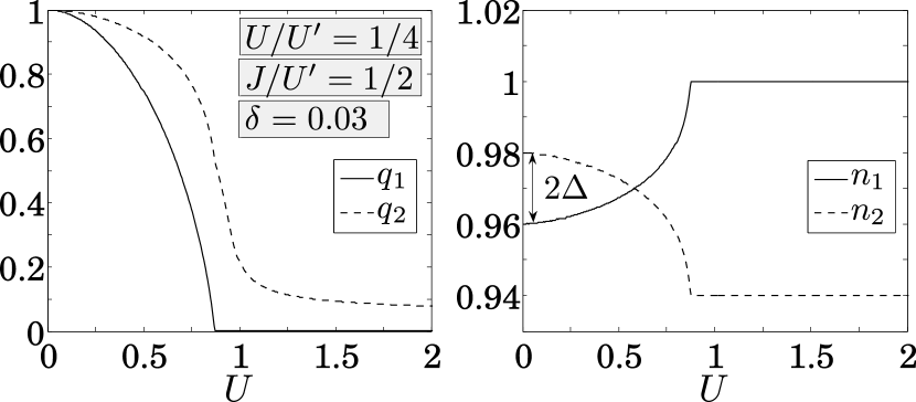
Figure 12: Band-renormalization factor $q_{\alpha}$ for finite hole doping $\delta=0.03$ and the charge distribution of the two bands for a fixed ratio $U^{\prime}/U=1/2$ and $J/U=1/4$.

As a representative example we show in Fig. 12 the band-renormalization factors $q_{\alpha}$ and the charges $n_{\alpha}$ for fixed ratios $U^{\prime}/U=1/2$ and $J/U=1/4$ and given doping $\delta=0.03$. Let us first look at the noninteracting case, $U=0$. The ground-state energy per site in this case is

$$E_{\mathrm{G}}=\bar{\varepsilon}_{1}^{o}(1-\delta_{1}^{2})+\bar{\varepsilon}_{2}^{o}(1-\delta_{2}^{2})$$ (17)

where $\delta_{\alpha}$ is the deviation from half filling in band $\alpha$ and $\bar{\varepsilon}_{\alpha}^{o}$ the average kinetic energy per site in band $\alpha$ for a half-filled band. Since $\bar{\varepsilon}_{\alpha}^{o}$ is proportional to the bandwidth $D_{\alpha}$ we find that the kinetic energy is optimized by choosing the charge imbalance $\Delta=(n_{1}-n_{2})/2=(D_{1}-D_{2})/(D_{1}+D_{2})\delta$. For $\delta=0.03$ and $D_{1}/D_{2}=1/2$ this gives the value $\Delta=-0.01$ as seen in Fig. 12. Thus, for $U=0$, the narrow band serves as a charge reservoir that allows to bring the broader band closer to half filling. With increasing interaction the Coulomb energy causes a transfer of electrons from the wide band to the narrow band in order to reduce the intraorbital repulsion. Thus, with increasing interaction strength, the broader band serves as a charge reservoir. This gives rise to a half-filled band ($\Delta=\delta$) at a certain interaction strength and to an OSMT. The metallic behavior of the second band is due to the finite hole doping and we find $q_{2}=2\delta$ up to first order in $\delta$ in the atomic limit $\bar{\varepsilon}_{\alpha}/U\rightarrow 0$ Lavagna:90 .

5 Discussion

5.1 Comparison to known results at half filling

On the mean-field level of the slave-boson approach we investigated the Mott transition in the two-band Hubbard model with different bandwidths and confirmed several aspects of previous work. As reported by several authors Liebsch:03 ; Liebsch:04 ; Koga:04 ; Koga:04b ; Koga:04c ; deMedici:05 ; Ferrero:05 ; Arita:05 ; Knecht:05 ; Liebsch:05 ; Inaba:05 we observe the OSMT and consequently an intermediate phase where only the narrow band is insulating whereas the wide band still has metallic properties.

Our mean-field calculations predict that for $U=U^{\prime}+2J$ the OSMI phase is limited to a small parameter regime in the $U$-$U^{\prime}$ phase diagram which is characterized by a rather high value of $J$ (Fig. 5). Compared to the phase diagram shown in Koga:04 the strength of the OSMI phase is strongly reduced. In view of our treatment of the Hund’s rule coupling this can be expected. As pointed out in Koga:04b ; deMedici:05 ; Liebsch:05 ; Knecht:05 the pair-hopping and the spin-flip term of the full Hund’s rule coupling lead to a stabilization of the OSMI phase. Since these terms are omitted in our calculations (and also in previous QMC studies Liebsch:03 ; Liebsch:04 ; Knecht:05 ) the OSMI phase is strongly reduced. Nevertheless, also with an Ising like Hund’s rule coupling we can clearly resolve a sequence of individual Mott transitions in our slave-boson approach.

In addition, we showed that on the mean-field level the PM-OSMI transition is second-order whereas the OSMI-MI and PM-MI transitions are first-order. Near these transitions there coexist two different solutions and the energy crossing results in a first-order transition (Fig. 7). The same behavior was reported in Ferrero:05 in the framework of the Gutzwiller approximation. Different results were found within other methods but non of the used methods is rigorous and the order of the transitions remains an open problem. Furthermore, temperature as well as pair-hopping and spin-flip terms might affect the order of the phase transitions Liebsch:05 .

For the case $U=U^{\prime}$ and $J=0$ orbital fluctuations lead to a stabilization of the metallic phase and for a fixed ratio of the bandwidths $D_{1}/D_{2}=1/2$ a joint second-order transition is observed (Fig. 3(b)). For the case of two bands of much different bandwidths, $D_{1}\ll D_{2}$, the Gutzwiller approximation and related mean-field theories predict the existence of an OSMI if the ratio $D_{1}/D_{2}$ is below a critical value. This was first reported in Ferrero:05 ; deMedici:05 . DMFT calculations give clear evidence that the localized band is not a conventional Mott insulator but has spectral weight down to arbitrarily small energies. However, an instability toward an orbitally ordered phase might play an important role for $U=U^{\prime}$ and should also be taken into account in future investigations.

5.2 Results for shifted bands

In real materials different atomic orbitals are usually not degenerate so that each band has non-commensurate filling. This extension of our model has lead to a considerably richer phase diagram. Such models correspond to the situation found in $\hbox{Ca}_{2-x}\hbox{Sr}_{x}\hbox{RuO}_{4}$ which has three bands of partial filling. This material has been an initial motivation for the study of the OSMT Anisimov:02 . Anisimov and coworkers proposed that the Ca-Sr substitution varies band parameters which in the end leads to a Mott transition in two of the three bands Anisimov:02 . A further example which belongs likely to this class is the compound FeSi. This compound is a small gap semiconductor FeSi:02 . On the other hand, replacing Ge for Si gives rise to a ferromagnetic metal. Alloying FeSi_1-xGe_x allows in principle for a continuous change of the band parameters such that the transition can be observed. However, the transition is simultaneous accompanied by an abrupt transition in the crystal lattice FeSiGe:03 .

Within the mean field approximation we find the following situation. For small crystal field splitting an OSMT is observed. In general, the Mott transition is shifted to higher values of the interaction parameters. Due to the crystal field, a band insulating phase and, in the presence of the Hund’s rule coupling, also a ferromagnetic phase appear in the phase diagram (Fig. 8). In the ferromagnetic phase, a few electrons populate the upper band with a finite net magnetization. For the case $U=U^{\prime}$ and $J=0$ we find a totally different behavior (Fig. 10). With increasing field, the metallic phase is less stable because the crystal field suppresses orbital fluctuations, similar to a finite $J$, by breaking the degeneracy of the local states.

For finite doping our calculations suggest that there is in general a Mott transition in the narrow band for not too strong doping. Although strongly correlated, the second band stays metallic due to the finite doping. This was also reported in Koga:04 .

5.3 Conclusions

In summary, the mean-field theory based on the slave-boson approach of Kotliar and Ruckenstein gives results which are in good qualitative agreement with DMFT calculations. While we restricted ourselves to density-density interactions, our discussion provides a simple physical picture in a wide range of parameters. The transverse spin coupling and the on-site interorbital pair hopping had to be dropped for practical reasons. Nevertheless, we believe that the effects are rather of quantitative than qualitative nature.

The method used emphasizes the on-site correlation and intersite correlations remain treated at a minor level only. Thus we have ignored symmetry breaking instabilities which double the size of the unit cell, such as antiferromagnetic instabilities or orbital order. These orders depend strongly on the detailed band structures and coupling topologies. In most of our discussion, however, we neglected the band structure aspect. Obviously nesting properties would play a major role in this context. Generic bands without nesting, however, follow more likely the ”plain” behavior of the simple flat density of states models that we discussed here. It would be interesting in future studies to extend the scheme by including also band structure effects and the related ordering phenomena.

- (1) A. Liebsch, Phys. Rev. Lett. 91, 226401-1 (2003)
- (2) A. Liebsch, Phys. Rev. B 70, 165103 (2004)
- (3) A. Liebsch, cond-mat/0505393
- (4) A. Koga, N. Kawakami, T. M. Rice, and M. Sigrist, Phys. Rev. Lett. 92, 216402-1 (2004)
- (5) A. Koga, N. Kawakami, T. M. Rice, and M. Sigrist, Physica B 359, 1366 (2005)
- (6) A. Koga, N. Kawakami, T. M. Rice, and M. Sigrist, Phys. Rev. B 72, 045128 (2005)
- (7) K. Inaba, A. Koga, S. Suga, and N. Kawakami cond-mat/0506150
- (8) L. de’ Medici, A. Georges, and S. Biermann, cond-mat/0503764
- (9) M. Ferrero, F. Becca, M. Fabrizio, and M. Capone, cond-mat/0503759
- (10) R. Arita and K. Held, cond-mat/0504040.
- (11) C. Knecht, N. Blümer, and P. G. J. van Dongen, cond-mat/0505106
- (12) V. I. Anisimov, I. A. Nekrasov, D. E. Kondakov, T. M. Rice, and M. Sigrist, Eur. Phys. J. B 25, 191 (2002)
- (13) A. Liebsch, Europhys. Lett. 63, 97 (2003)
- (14) C. Castellani, C. R. Natoli, and J. Ranninger, Phys. Rev. B 18, 4945 (1978)
- (15) G. Kotliar and A. Ruckenstein, Phys. Rev. Lett. 57, 1362 (1986)
- (16) W. F. Brinkman and T. M. Rice, Phys. Rev. B 2, 4302 (1970)
- (17) M. C. Gutzwiller, Phys. Rev. Lett. 10, 159 (1962)
- (18) M. C. Gutzwiller, Phys. Rev. 137, A1726 (1964)
- (19) L. D. Landau, Zh. Eksp. Teor. Fiz 30, 1058 (1956)
- (20) P. Dietrich, Ph.D. thesis, Würzburg, 1994.
- (21) D. Vollhardt, Rev. Mod. Phys. 56,99 (1984)
- (22) M. Lavagna, Phys. Rev. B 41, 142 (1990)
- (23) V.I. Anisimov et al., Phys. Rev. Lett. 89, 257203 (2002)
- (24) S. Yeo et al, Phys. Rev. Lett. 91, 046401 (2003)