Elastic lines on splayed columnar defects studied numerically

Abstract

We investigate by exact optimization method properties of two- and three-dimensional systems of elastic lines in presence of splayed columnar disorder. The ground state of many lines is separable both in 2d and 3d leading to a random walk -like roughening in 2d and ballistic behavior in 3d. Furthermore, we find that in the case of pure splayed columnar disorder in contrast to point disorder there is no entanglement transition in 3d. Entanglement can be triggered by perturbing the pure splay system with point defects.

I Introduction

Transport properties of type-II superconductors are influenced by the presence of various kinds of disorder Blatter . Pinning of vortex lines hinders their motion, which, in response to an applied current, causes dissipation. From the practical point of view it is highly desirable to avoid the appearance of vortex creep which gives rise to a finite resistivity. It was proposed by Hwa et al. Hwa that splayed columnar defects resulting from heavy ion irradiation of superconducting samples, would significantly enhance the vortex pinning, and thus reduce the vortex creep leading to a higher critical current density $j_{c}$. An additional important aspect might be the inhibition of vortex motion due to forced entanglement induced by the disorder entgl .

The predictions concerning $j_{c}$ have been been verified in experiments on samples with different sources of splayed defects K-E ; Civale ; Kwok . Kwok et al. Kwok reported that well above the matching field $B_{\phi}$, where the density of vortices equals to the density of columnar defects, the irreversibility line of sample with splay is below of the one without splay defects. As an evidence of strong entanglement above the matching field it was discovered Kwok that although the irreversibility is decreased in samples with splay defects values of $j_{c}$ are still greatly increased compared to unirradiated samples. On the other hand the comparison of samples with one and two families of splay defects did not reveal any differences in the values of $j_{c}$ Hebert . Molecular dynamics simulations for $B>B_{\phi}$ show the increase of $j_{c}$ in the samples with splay disorder Palmer ; Olson . The authors of Olson have also performed simulations on samples with $B<B_{\phi}$ for which they obtained a milder enhancement of $j_{c}$. On the basis of these observations they suggested that in the case $B>B_{\phi}$ the additional increase of $j_{c}$ is due to vortex entanglement.

The ground state properties of an ensemble of flux lines in such disordered environments has never been investigated before. Single flux line properties in the presence of tilted columnar defects at zero temperature were studied by Lidmar et al. Lidmar . They show that the behavior of the lines depends on the energy distribution of the lines. This is manifested in roughening, or mean-square displacement as a function of sample height $H$,

$$w^{2}(H)=\langle\mathrm{\bf r}(z)^{2}\rangle_{z}-\langle\mathrm{\bf r}(z)\rangle_{z}^{2}\sim H^{2\zeta}.$$ (1)

Here $z$ is the distance along the height direction, and $r$ the transverse displacement. According to Lidmar et al. the roughness exponent $\zeta$ is sensitive to the shape of the distribution of the tilt angle and the energy distributions of the defects Lidmar . For instance with an opening angle of $90^{\circ}$ and for a uniform energy distribution the roughness exponent in 2d is $\zeta=3/4$, in contrast to the point-disorder result $2/3$ Halpin . In samples with a fixed starting point a single line has the following geometry. It occupies a splay defect until a jump to a energetically more favorable one takes place. The lines undergo jumps from splay defect to splay defect so that the average distance between two successive jumps grows as $\Delta z\sim z$ Lidmar . Thus though the jump density decreases with growing $z$ the roughening exhibits a non-trivial scaling.

The natural question arises how the single-line physics outlined above changes in the presence of many interacting lines, at a constant line density $\rho$. In this paper we study this in both two (2d) and three dimensions (3d). There are studies of the role of disorder in two-dimensional samples Bolle , while the three-dimensional case corresponds to bulk superconductors. We find that at finite line densities the physics changes in particular as the roughening of lines is concerned: the roughness exponent becomes $\zeta=1/2$ in 2d and $\zeta=1$ in 3d. The ballistic behavior of the lines leads to the absence of true entanglement in 3d.

This paper is organized as follows. In Sec. II we explain the details of our numerical model. The scaling of roughness is discussed in Sec.III. We also study in Sec. IV if inserting a new line causes rearrangements in the configuration of previously inserted lines, ie. as the density is increased. The results shown in Sec. V demonstrate that in pure splay disorder lines do not entangle. Entanglement can be induced by perturbing splay with point disorder. The summary and discussion are presented in Section VI.

II Model

We consider the following model of a system of interacting lines in a two- or three-dimensional disordered environment: The lines live on the bonds of a graph consisting of an ensemble of splayed columns embedded in a box with a width $L$ and a height $H$ (Fig. 1). Each column is described with a transverse coordinate $\mathrm{\bf r}(z)$ at height $z$ from the bottom level:

$$\mathrm{\bf r}(z)=\mathrm{\bf r}_{0}+\mathrm{\bf a}\,z$$ (2)

where $\mathrm{\bf r}_{0}$ is a random point on the basal plane and $\mathrm{\bf a}$ is a randomly chosen variable that defines the magnitude and the orientation of the tilt of a given column.

Figure 1: Schematic figure of the graph consisting of splayed columns in two and three dimensions. In the latter case note the two additional bonds connecting the columns.

The number of columnar defects $M$ is set to $M=L$ and $M=L^{2}$ in two and three dimensions respectively. The average distance between two nearby columnar defects defines the in-plane length unit of the model. The lines enter the system at the bottom plane ($z=0$) and they exit at the top plane ($z=H$), and we use both fixed and free entrance points, and free exit points. The case of a fixed entry point and a free exit point is that considered by Lidmar et al. for a single line Lidmar , who discuss an experimental scenario for the same. Also rough enough surface could pin the end points of flux lines. Strong pinning along large surface steps has been reported in Ref. dai . More recent experimental results fil indicate that surface pinning have measurable effects on the flux lattice dynamics.

In this paper we study the case where the columns have a random, uniformly distributed orientation within a cone with a fixed opening angle. In our model changing the opening angle of the cone is equivalent to a rescaling of the system height, for which reason we consider only the opening angle of $90^{\circ}$.

The number $N$ of lines threading the sample is fixed by the prescribed density $\rho=N/M$. Within this version of the model number of lines cannot exceed the number of columns, which means in the case of splay disorder that $B<B_{\phi}$. The graph could be in principle modified such that lines can traverse the system also between the columnar defects which would correspond to $B>B_{\phi}$.

In the transverse directions we use both periodic and open boundary conditions. In the latter case the defects crossing the boundary are cut such that lines cannot follow them across the system boundaries. Note that one can not let flux lines escape from truly open boundaries since the line density would decrease with $z$, the longitudinal coordinate. In order to avoid correlations in systems with $H>L$ we first construct a graph of size $H^{d}$ from which we cut a piece of size $L$.

In 2d lines can change defects only at their crossings and in 3d when the defects are close enough to each other. In 3d columns are connected by introducing an extra segment between the lines at the shortest mutual distance whenever this distance is shorter than a fixed value $r_{c}$. When $r_{c}$ is kept relatively small compared to the average distance between the columnar defects the choice of the energy cost of the bond connecting two defects can be arbitrary. We choose zero energy cost and $r_{c}=1.4$. We have also checked the value $r_{c}=0.5$ which did not change the results.

We model the disordered environment by assigning a random (potential) energy $e_{ij}=r_{ij}u$ to each bond $(i,j)$, where $r_{ij}$ is the Euclidean length of the bond and $u$ is a random number which determines the type of disorder. In the case of splay disorder the random variable $u$ is drawn independently for each column such that bonds along a given column share the same value of $u$. Point disorder is modeled with a similarly constructed graph. The only difference is that $u$ is drawn independently for each bond which destroys the correlations along the columns. For point disorder we use uniformly distributed $u$ and for splay disorder the following distribution in order to make comparisons to single line results by Lidmar et al. Lidmar :

$$P(u)=\nu u^{\nu-1}\,,$$ (3)

for $0<u<1$ and otherwise $P(u)=0$. With $\nu=1$ this reduces simply to a uniform distribution.

For computational convenience we focus on the short screening length limit screening . We restrict ourselves to hard-core interactions between the lines, which means that their configuration is specified by bond-variables $x_{ij}\in\{0,1\}$, $x_{ij}=1$ indicating that a line segment occupies a bond between nodes $i$ and $j$, and $x_{ij}=0$ indicating that no line segment occupies this bond. The total energy of the line configuration is given by

$${\mathcal{H}}=\sum_{(ij)}x_{ij}\cdot e_{ij}\,,$$ (4)

where the summation is performed over all bonds. The corresponding Hamiltonian in a continuum limit is given by the following formula:

$${\mathcal{H}}={\displaystyle\sum_{i=1}^{N}}{\displaystyle\int_{0}^{H}dz}\Bigl{\{}\frac{\gamma}{2}\left[\frac{d{\bf r}_{i}}{dz}\right]^{2}+V_{r}[{\bf r}_{i}(z),z]$$

$$+\sum_{j(\neq i)}V_{\rm int}[{\bf r}_{i}(z)-{\bf r}_{j}(z)]\Bigr{\}}\;,$$ (5)

where ${\bf r}_{i}(z)$ denotes the transversal coordinate at longitudinal height $z$ of the $i$-th flux line. The interactions $V_{\rm int}[{\bf r}_{i}(z)-{\bf r}_{j}(z)]$ are hard core repulsive and the disorder potential $V_{r}[{\bf r}_{i}(z),z]$ is $\delta$-correlated in the case of point disorder and strongly correlated along columns in the case of columnar disorder. The elastic energy is mimicked in our numerical model by the positivity of all energy costs per unit length, which ensures for instance the minimization of the line length in the absence of randomness.

At low temperatures the line configurations will be dominated by the disorder and thermal fluctuations are negligible. Therefore we restrict ourselves to zero temperature and focus on the ground state of the Hamiltonian (4). Computing the ground state now corresponds to finding $N$ non-overlapping directed paths traversing the graph along the bonds from bottom to top. One has to minimize the total energy of the whole set of the paths and not of each path individually (n.b.: already the two-line problem is actually non-separable twoline ). For a single line problem the lowest energy path can be found straightforwardly with Dijkstra’s shortest path algorithm. In the case of many lines Dijkstra’s algorithm is applied successively on a residual graph instead of the original graph opt-review as illustrated in Fig. 2. In the residual graph the properties of occupied bonds are modified as follows: If $x_{ij}=1$ we set $e_{ij}^{\rm residual}=-e_{ij}$, i.e. negative, and require that the direction of a new path must be in the opposite direction with respect to the direction of previously inserted paths. The path segments with two opposite directions on a given bond are canceled. For details see opt-review .

Figure 2: Schematic figure of adding lines to the graph. (a) The ground state of a single line with arrows indicating the direction of the optimal path. (b) The bold line is the optimal path from bottom to top in the residual graph. The residual graph is constructed by changing the energy costs of the bonds to negative along the dotted line. In addition, the direction of paths in the residual graph on the dotted bonds must be opposite to the direction of the previously inserted path shown in (a). (c) The final line configuration after the path segments with opposite directions are canceled.

Although the lines cannot occupy the same bond of the lattice they may touch in isolated points if the nodes in these points have more than three neighbors. This is now the case only in 2d as exemplified in Fig.1. Since we want to calculate the roughness of lines we need to determine the individual lines, for which we use a local rule. In 2d the line identification is unambiguous if we simply require that the lines cannot cross.

In our model flux lines are confined to the defects with no possibility to enter the bulk (except in 3d if the jumps from one defect to another are counted as such). We also tested the case where a homogenous bulk between the splayed defects is represented by a set of densely packed columnar defects with zero tilt and with a constant energy cost per unit length. Here, after a flux line has found a splayed defect with a lower energy cost per unit length in $z$-direction compared to the one in the bulk one recovers the pure splay disorder behavior. Thus, including the possibility for lines to travel also in the bulk introduces another crossover length. We have checked numerically that this scenario holds. After a cross-over system size, which depends on the ratio of the energy costs in the bulk and on the defects, for single line systems we obtain the roughness exponents of pure splay disorder.

In many line systems with a fixed ratio between the number of splay defects and the number of inserted flux lines it is not guaranteed that all lines can find a defect which is energetically more favorable than the bulk. Depending on the energy cost of the bulk there can be only a fraction of splayed defects which are energetically more favorable compared to the bulk. If the number of such defects is smaller than the number of flux lines there will be a fraction of lines $f_{bulk}$ that stay in the bulk throughout the whole sample. As a function of the energy cost per unit length in the bulk $u_{bulk}$ this scales like $f_{bulk}=g(u_{bulk}/\rho^{\alpha})$ with $g(x)$ a scaling function that decreases monotonically from $1$ at $x=0$ to zero for $x=1$ and $\alpha$ depending on the shape of the energy distribution of the splayed defects (Eq.(3)).

Since the lines staying in the homogenous bulk have no transverse fluctuations our central results on the geometrical properties of flux line systems in splay disorder are not expected to change qualitatively.

III Roughness of the ground state

In this section we focus on the scaling of the average roughness $w$, i.e. the amount of transverse wandering of the lines. The mean square displacement the $i$-th line is $w^{2}_{i}=\langle\mathrm{\bf r}_{i}(z)^{2}\rangle_{z}-\langle\mathrm{\bf r}_{i}(z)\rangle_{z}^{2}$ where $\mathrm{\bf r}_{i}(z)$ is the transverse coordinate of the line $i$ at the distance $z$ from the bottom level and $\langle\mathrm{\bf r}(z)\rangle_{z}=\frac{1}{H}\int_{0}^{H}\mathrm{\bf r}(z)\,dz\,$ denotes the average along the line from the bottom $z=0$ to the top $z=H$. We define $w^{2}$ as the disorder average of $w^{2}_{i}$ averaged over all lines.

In the case of point disorder our model is in the same universality class as the directed polymer model according to which the roughness of one line scales as $w\sim H^{\zeta}$ with well known exponents $\zeta_{2d}=2/3$ and $\zeta_{3d}\approx 5/8$ in two and three dimensions respectively Halpin . In 2d the steric repulsion between the lines leads to collective rearrangement of the lines which yields a logarithmic growth of the roughness. In 3d lines can wind around each other which suppresses the repulsion resulting in a random walk-like behavior of lines rough .

For splay disorder, we propose the following simple scenario. At small $z$ lines do not see each other and exhibit single line behavior. Beyond some value of $z$, which depends on the density $\rho$, the lines cannot further optimize their configurations and stay on the same defects. This leads to a linear growth of the roughness, $\zeta=1$ in 3d due to ballistic behavior. The same arguments on the structure of the optimal line configuration hold also for 2d. However, in 2d splayed defects can cross each other while the individual flux lines are identified such that they do not cross the other flux lines. Thus, in 2d one has effectively system of hard-core repulsive random walks resulting in $\zeta=1/2$. Thus one would expect a roughness scaling form

$$w(L,H)\propto L^{\zeta}f(H/L),$$ (6)

where $f(x)$ is a scaling function. In both 2d and 3d, this scenario is independent of the splay energy distribution.

Fig. 3 shows the correctness of this proposition in 3d. One can see from Fig. 3(a) that the roughness of many line systems grows linearly $w\sim H$ with no dependence on the energy distribution of the defects. According to the data collapse in Fig. 3(b) the saturation roughness and the saturation height grow linearly with the system width $L$, cf. with Eq.(6).

In 2d there is a collective regime, where the lines exhibit random walk like -behavior as suggested above. Fig. 4(a) shows that the roughness grows asymptotically like $w\sim H^{0.5}$ for both values of $\nu$. The data collapse shown in Fig. 4(b) gives the random walk like scaling also for the saturation roughness in agreement with Fig. 4(a). Close to the system boundaries the roughness of the lines is suppressed (due to the way the line identification is made in 2d) which shows up in the scaling of small system widths $L$.

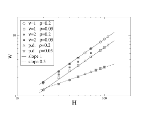
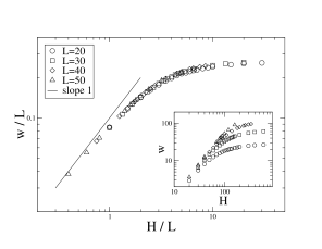
Figure 3: Doubly logarithmic plots for the roughness $w$ of multi-line systems in 3d. Top: Roughness vs. system height $H$ ($L=H$) for different values of line density $\rho$ and for two defect energy distributions ($\nu=1,\,2$); lines have fixed starting points. For comparison are shown also the roughness for point disorder (labeled as “p.d.”). Bottom: Scaling plot for the roughness with fixed system widths for $\rho=0.2$ and $\nu=1$, the un-scaled data are shown in the inset. At this line density the difference between the data with fixed and free starting points is undistinguishable.

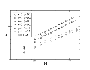
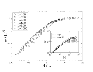
Figure 4: Double logarithmic plots for the roughness $w$ of multi-line systems in 2d. Top: Roughness vs. system height $H$ ($L=H$) for different values of line density $\rho$ and for two defect energy distributions ($\nu=1,2$); lines have fixed starting points. Bottom: Scaling plot of the roughness with fixed system widths $L$ and fixed starting points with line density $\rho=0.1$ and $\nu=1$.

IV Separability of the ground state

We define that the ground state configuration of $N$ lines is separable if it can be obtained by adding successively flux lines to the system without modifying the configurations of the previous lines. This can be checked from the successive shortest path algorithm: whenever segments of flux lines are canceled in the residual graph this implies that adding a line changed the previous configuration (see Fig. 2). Hence we focus on such segments or bonds and calculate the sum of the energy costs $E_{s}=\sum e_{ij}$ of such bonds and use it as a measure of the separability. When $E_{s}=0$ no flux is canceled due to possible rearrangements of line configuration. This means that one has fully separable ground state.

In the case of (splayed) columnar disorder it is obvious that with periodic boundary conditions and the full freedom of choosing the most favorable starting point the lines pick up the defects in the order of their total energy cost from the source to the target. Hence, no rearrangements of flux line configurations is needed. Introducing the boundaries or any other distortions to the pure columnar disorder reduces the separability of the ground state.

In Fig. 5 we demonstrate the difference between the separability of the ground states of splay and point disorder. We consider $L\times H$ systems in two dimensions with periodic boundary conditions in the direction perpendicular to the $z$-axis. In the case of splay disorder $E_{s}$ saturates at a particular system height, because line rearrangements do not take place at greater $z$. Thus $E_{s}$ divided by the system volume goes to zero with increasing $H$, implying separability. Compare with the fact that $E_{s}$ is linear in $H$ in the case of point disorder, indicating non-separability. We calculated $E_{s}$ also in three dimensions and observed the same behavior as in the 2d case as is depicted in Fig. 6.

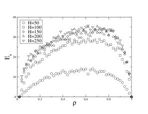
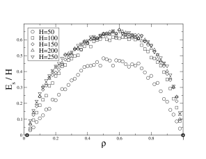
Figure 5: A measure of the separability of the ground state in 2d, periodic boundaries, fixed starting points, L=50. Top: splay disorder, $E_{s}$ saturates as $H$ grows. Bottom: point disorder, $E_{s}$ grows linearly with $H$.

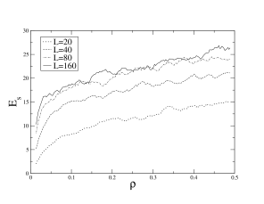
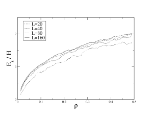
Figure 6: Same as Fig. 5, now in 3d with L=20 and line density only up to $\rho=0.5$ due to increased computational costs. The data is smoothened by taking running averages of each 10 subsequent data points.

V Entanglement

In 3d lines can wind around each other resulting in topologically non-trivial configurations which we analyze here by computing the winding angle of all line pairs as indicated in Fig. 7 (c.f. Drossel ). We define two lines to be entangled when their winding angle becomes larger than $2\pi$ entgl . This provides a measure for topological entanglement Samokhin , since a topologically entangled pair can not be separated by any linear transformation in the basal plane (i.e. the lines almost always would cut each other, if one were shifted).

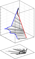
Figure 7: (a) Definition of the winding angle of two flux lines: For each z-coordinate the vector connecting the two lines is projected onto that basal plane. $z=0$ gives the reference line with respect to which the consecutive vectors for increasing $z$-coordinate have an angle $\phi(z)$. Once $\phi(z)>2\pi$ the two lines are said to be entangled. (b) Top : A configuration of six entangled lines with splay disorder. Bottom: The projection of the line configuration on the basal plane, defining a connected cluster. (c) Six entangled lines with point disorder.

Sets or bundles of pairwise entangled lines are defined such that a line belongs to a bundle if it is entangled at least with one other line in the set. In the case of point disorder such bundles are spaghetti-like — i.e. topologically complicated and knotted sets of one-dimensional objects which grow with increasing system height leading finally to one giant bundle. In entgl it was shown that for point disorder there is a sharp transition from an non-entangled phase without giant bundle to an entangled phase: The probability $P_{perc}$ for having an entangled bundle of lines that spans the system in the transverse direction jumps from 0 to 1 at a critical height $H_{c}$ in the infinite system size limit ($L\to\infty$), and is described by the following finite size scaling form

$$P_{perc}=p(L^{1/\nu}(H-H_{c}))\;.$$ (7)

One implication of this scaling form is that the location of the jump of $P_{perc}$ from 0 to 1 for finite size $L$ saturates at some value $H_{c}$ in the limit $L\to\infty$, another that the jump width decreases with $L$.

This appears not to be the case for splay disorder. As one can see from Fig. 8(a) $H_{c}$ does not saturate for the computationally accessible system sizes ($L\lesssim 120$). From the inset one can also see that the width of the transition does not decrease.

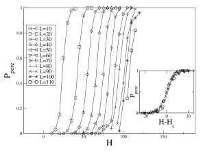
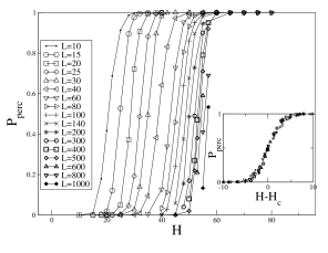
Figure 8: Percolation probability as a function of the height of the system $H$: (a) splay disorder and (b) ballistic random walk. Insets: data shifted with $H_{c}$. For both the transition width does not change, there is only a shift of the jump $H_{c}(L)$.

For a comparison, we use the following model consisting of random walks embedded into a box of size $L\times L\times H$. Since the lines typically change their direction only in the vicinity of the boundaries we consider ballistic random walks. They start from a random point at the basal plane and evolve towards the top level with a random tilt angle taken from the same distribution as for the splayed columns. When the random walk meets the system boundary it is assigned a new tilt angle. This is repeated until the path hits the top of the system. This model corresponds to the high density limit where all defects are occupied, i.e. $B=B_{\phi}$.

We calculate the mutual winding angles and check for entanglement as before. By comparing Fig. 8(a) and Fig. 8(b) one observes no qualitative differences in the dependence of the percolation probability $P_{perc}$ from the system height $H$. No saturation is found for percolation height $H_{c}$ as the system width is increased, though the growth is extremely slow. According to our numerical results the transition height appears to grow asymptotically like $H_{c}\sim(\log L)^{a}$ with $a$ close to 0.5 (Fig. 10).

The inset of Fig. 9 shows the relative size of the percolating bundle $n_{perc}/n_{tot}$ for the data of Fig. 8(a). It tends to zero for increasing system size also for $H>H_{c}$. This is in contrast to what happens for conventional percolation where $n_{perc}/n_{tot}=0$ exactly at the threshold and then increasing as $\sim(H-H_{c})^{\beta}$ with the critical exponent $\beta$. Fig. 9 shows the distribution $P(k)$ of the number of lines $k$ with which a given line is entangled (i.e. wind around it by an angle larger than $2\pi$). One sees that the probability distribution $P(k)$ is almost identical in the cases of splay disorder and ballistic random walks, whereas $P(k)$ for point disorder is much narrower.

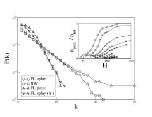
Figure 9: A plot with logarithmic $y$-axis of distribution of the degree of lines’ entanglement $P(k)$. $k$ is defined as the number of lines with which a given line is entangled. The following data sets are shown: flux lines in splay disorder with L=100, H=115 (ovals); ballistic random walks with L=100, H=39 (squares); flux lines in point disorder with L=100, H=48 (triangles up); flux lines in splay disorder with fragmentation L=100, H=70 (triangles down). The system heights are chosen so that the system is in the vicinity of the entanglement transition. Inset: strength of the percolating cluster of flux lines in splay disorder is plotted in a linear scale vs. system height $H$ for different system widths, L=30 (ovals) … 110 (filled ovals).

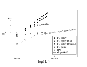
Figure 10: A loglog plot of estimated critical system heights $H_{c}$ vs. logarithm of the system width $L$. From top: flux lines (FL) with free and fixed (fix) starting points in splay disorder; flux lines in splay disorder with fragmentation (fragm.) and in point disorder; ballistic random walks (RW), solid line is a fit to few last data points.

We conclude that in the case of splayed columnar disorder the spanning bundles are formed mostly by few lines which bounce from the boundaries. Thus, there is no entanglement percolation transition in the case of splay disorder and no giant entangled cluster in the thermodynamic limit.

This behavior changes when the splay disorder is perturbed with attractive or repulsive point defects. Here we discuss results for relatively weak attraction. The energy costs per unit length for a fraction $f$ of the bonds are now set to $u=0.5$ whereas the rest of the bonds are as before. Fig. 11 shows the behavior of the percolation probability corresponding to $f=0.1$. It indicates now the presence of an entanglement transition following the conventional percolation scenario (Eq. (7)). The transition height $H_{c}$ saturates in the limit $L\to\infty$ (Fig. 10) and the data obey finite size scaling with the correlation length exponent $\nu=4/3$ of the 2d percolation problem.

The fraction $f$ tunes the typical length that a given line stays on one defect. When this length exceeds the one needed to traverse the system in the lateral direction one observes the properties of pure splay disorder. Consequently as $f$ is decreased one needs increasingly larger system sizes in order to observe the percolation transition. The strength and the nature – repulsive or attractive – of the perturbing point disorder only changes the crossover size of the system as long as the perturbation is strong enough to induces lines to change the defects. However, due to computational limitations we did not attempt to find whether there is a threshold value for strength of point disorder below which the lines cannot be entangled also in the infinite system size limit.

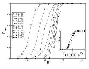
Figure 11: Percolation probability as a function of the height of the system $H$ for splay disorder with fragmentation. Inset: corresponding scaling plots, Eq. (7). Fragmentation causes the sharpening of the transition width with growing $L$ and data scales with the 2d percolation correlation length exponent $\nu=4/3$.

VI Summary and discussion

The ground state of a multi-line system with splay disorder has four different phases as a function of the system height $H$. For small values, there is first a cross-over from trivial behavior to the single-line ground state roughening as lines start to jump between columnar defects. For intermediate $H$, one observes the collective regime where $\zeta$ depends on dimension but not on the splay energy distribution. This arises when the lines transverse wandering becomes of the same order of magnitude as the average line distance. Finally, there is the cross-over to saturation for $L$ finite. The exponent values are a random walk-like $\zeta_{2d}=1/2$ and a ballistic-like $\zeta_{3d}=1$. The cross-over between the collective and single-line scalings is visible in our 2d data. In 3d, this is not possible for numerical restrictions. Note the fact that the 3d single line exponent (which varies with the energy distribution) is smaller than the collective one.

We have also considered the separability and entanglement, to look at the other aspects of these systems as $H$ is varied. The former measures the collective aspects of the line configuration, which are most pronounced for $z$ small. In contrast to the 3d point disorder case, the winding of lines around each other is suppressed, leading to the absence of entanglement in the thermodynamic limit. In the context of our current model, this means that for low line densities ($B<B_{\phi}$) the enhanced pinning expressed by increased critical current, is not a collective effect.

The results for the splay disorder are not expected to change qualitatively when the flux lines are allowed to enter the homogenous bulk between the defects. As discussed in end of Sec. II in this case there will be a fraction of lines staying in the bulk throughout the sample. Since these lines have no transverse fluctuations they reduce the average roughness by a constant factor.

Our numerical results suggest that inserting point-like defects into splay disorder may even further enhance the flux line pinning as the entanglement transition of flux lines is recovered. For large line densities ($B>B_{\phi}$) – where experiments Kwok imply entanglement – one could study the role of additional point disorder. This brings new complications, already for single lines. In the case of one attractive columnar defect competing with point disorder in 2d one finds only a localized line, whereas in 3d there a localization-delocalization transition Balents . Another study has found for a mixture of many columnar defects and point disorder sub-ballistic behavior Arsenin .

Lidmar et al. found by mixing in point disorder that in 2d splay disorder always dominates on the long length scales whereas in 3d it seems that strong enough fragmentation leads to point disorder behavior Lidmar . Here we briefly present a few possible scenarios associated with tuning the strength of point disorder with fixed strength of splay disorder: (i) At large enough system sizes point disorder will always dominate. (ii) There is a crossover from pure splay disorder behavior (no entanglement) to point disorder behavior. (iii) There is a third regime where lines take an advantage of both splay and point disorder leading possibly to more efficient entanglement than in the case of pure point disorder. This would be due to the large displacements along splayed defects. One can expect that the response of the system to point disorder perturbations depends on the line density. It would be interesting to find the full phase diagram including the optimal parameters from the point of view of entanglement.

- (1) G. Blatter, M. V. Feigel’man, V. B. Geshkenbaum, A. I. Larkin, and V. M. Vinokur, Rev. Mod. Phys. 66, 1125 (1994).
- (2) T. Hwa, P. Le Doussal, D. R. Nelson, and V. M. Vinokur, Phys. Rev. Lett. 71, 3545 (1993) .
- (3) V. Petäjä, M. Alava, and H. Rieger, Europhys. Lett. 66, 778 (2004).
- (4) L. Krusin-Elbaum, A. D. Marwick, R. Wheeler, C. Feild, V. M. Vinokur, G. K. Leaf, and M. Palumbo, Phys. Rev. Lett. 76, 2563 (1996).
- (5) L. Civale, A. D. Marwick, T. K. Worthington, M. A. Kirk, J. R. Thompson, L. Krusin-Elbaum, Y. Sun, J. R. Clem, and F. Holtzberg, Phys. Rev. Lett. 67, 648 (1991).
- (6) W. K. Kwok, L. M. Paulius, V. M. Vinokur, A. M. Petrean, R. M. Ronningen, and G. W. Crabtree, Phys. Rev. Lett. 80, 600 (1998).
- (7) S. Hébert, G. Perkins, M. Abd el-Salam, and A. D. Caplin, Phys. Rev. B 62, 15230 (2000).
- (8) C. M. Palmer and T. P. Devereaux, Physica C 341-348, 1219 (2000).
- (9) C. J. Olson, R. T. Scalettar, G. T. Zimányi, and N. Grønbech-Jensen, Phys. Rev. B 62, R3612 (2000).
- (10) J. Lidmar, D. R. Nelson, and D. A. Gorokhov, Phys. Rev. B 64, 144512 (2001).
- (11) T. Halpin-Healy and Y.-C. Zhang, Phys. Rep. 254, 215 (1995).
- (12) C. A. Bolle, V. Aksyuk, F. Pardo, P.L. Gammel, E. Zeldov, E. Bucher, R. Boise, D.J. Bishop, and D.R. Nelson, Nature (London) 399, 43 (1999).
- (13) H. Dai, J. Liu, and C. M. Lieber,Phys. Rev. Lett. 72, 748 (1994).
- (14) V. D. Fil, D. V. Fil, Yu. A. Avramenko, A. L. Gaiduk, and W. L. Johnson, Phys. Rev. B 71, 092504 (2005).
- (15) H. S. Bokil and A. P. Young, Phys. Rev. Lett. 74, 3021 (1995); C. Wengel and A. P. Young, Phys. Rev. B 54, R6869 (1996); J. Kisker and H. Rieger, Phys. Rev. B 58, R8873 (1998)
- (16) V. Petäjä, M. Alava, and H. Rieger, Int. J. Mod. Phys. C 12, 421 (2001).
- (17) M. Alava, P. Duxbury, C. Moukarzel, and H. Rieger, in Phase Transitions and Critical Phenomena, Vol. 18, edited by C. Domb and J.L. Lebowitz (Academic Press, 2000); A. Hartmann and H. Rieger, Optimization Algorithms in Physics (Wiley VCH, Berlin, 2002).
- (18) V. Petäjä, D.-S. Lee, M. Alava, and H. Rieger, J. Stat. Mech., 10010 (2004).
- (19) B. Drossel and M. Kardar, Phys. Rev. E 53, 5861 (1996).
- (20) K. V. Samokhin, Phys. Rev. Lett. 84 1304 (2000).
- (21) L. Balents and M. Kardar, Phys. Rev. B 49, 13030 (1994).
- (22) I. Arsenin, T. Halpin-Healy, and J. Krug, Phys. Rev. E 49, R3561 (1994).