Activated aging dynamics and negative fluctuation-dissipation ratios

Abstract

In glassy materials aging proceeds at large times via thermal activation. We show that this can lead to negative dynamical response functions and novel and well-defined violations of the fluctuation-dissipation theorem, in particular, negative fluctuation-dissipation ratios. Our analysis is based on detailed theoretical and numerical results for the activated aging regime of simple kinetically constrained models. The results are relevant to a variety of physical situations such as aging in glass-formers, thermally activated domain growth and granular compaction.

Glassy materials display increasingly slow dynamics when approaching their amorphous state. At the glass transition, where relaxation times exceed experimentally accessible timescales, they change from equilibrated fluids to non-equilibrium amorphous solids. In the glassy phase, physical properties are not stationary and the system ages Young . A full understanding of the non-equilibrium glassy state remains a central theoretical challenge.

An important step forward was the mean-field description of aging dynamics for both structural and spin glasses CugKur . In this context, thermal equilibrium is never reached and aging proceeds by downhill motion in an increasingly flat free energy landscape laloux . Two-time correlation and response functions depend explicitly on both their arguments, and while the fluctuation-dissipation theorem (FDT) does not hold it can be generalized using the concept of a fluctuation-dissipation ratio (FDR). This led in turn to the idea of effective temperatures CugKurPel97 , and a possible thermodynamic interpretation of aging CugKur ; FraMezParPel98 .

However, in many systems of physical interest, such as liquids quenched below the glass transition or domain growth in disordered magnets, the dynamics is not of mean-field type, displaying both activated processes and spatial heterogeneity FisHus86 ; Ediger00 . While some experiments and simulations CriRit03 nonetheless seem to detect a mean-field aging regime, theoretical studies have found ill-defined FDRs Cri-Vio , non-monotonic response functions newman ; nicodemi ; kr ; buhot , observable dependence FieSol02 ; MayBerGarSol , non-trivial FDRs without thermodynamic transitions BuhGar02 and a subtle interplay between growing dynamical correlation lengthscales and FDT violations barrat ; kennett ; experiments have also detected anomalously large FDT violations associated with intermittent dynamics exp . It is thus an important task to delineate when the mean-field concept of an FDR-related effective temperature remains viable.

Independently of this interpretation, FDRs have additionally been recognized as universal amplitude ratios for non-equilibrium critical dynamics. This makes them important markers for distinguishing dynamic universality classes. This area has seen a recent surge of interest CalGam .

Here we study kinetically constrained models, which are simple models for glassy systems with heterogeneous dynamics RitSol03 . We use them to study systematically the impact of activated, and therefore strongly non mean-field, dynamics on FDRs and associated effective temperatures. In addition, the dynamics of these models becomes critical at low temperatures, where dynamical lengthscales diverge. Our work therefore also pertains to the study of FDRs in non-equilibrium critical dynamics. We show that FDT violations retain a simple structure with well-defined FDRs in the activated regime, elucidate the physical origin of negative dynamical response functions, and predict the generic existence of negative FDRs for observables directly coupled to activated processes.

We focus mainly on the one-spin facilitated model of Fredrickson and Andersen FreAnd84 (FA model), defined in terms of a binary mobility field, $n_{i}\in\{0,1\}$, on a cubic lattice; $n_{i}=1$ indicates that a site is excited (or mobile). The system evolves through single-site dynamics obeying detailed balance with respect to the energy function $H=\sum_{i}n_{i}$. The dynamics is subject to a kinetic constraint that permits changes at site $i$ only if at least one nearest neighbor of $i$ is in its excited state. In any spatial dimension $d$, relaxation times follow an Arrhenius law at low temperatures RitSol03 ; WhiBerGar04 .

At low temperatures, $T<1$, the dynamics of the FA model is effectively that of diffusing excitations, which can coalesce and branch WhiBerGar04 ; SchTri99 . Such a problem can be described in the continuum limit by a dynamical field theory action with complex fields $\varphi(\boldsymbol{r},t)$, $\bar{\varphi}(\boldsymbol{r},t)$ WhiBerGar04 ; tauber ,

$$S=\int_{\boldsymbol{r},t}\bar{\varphi}(\partial_{t}-D\nabla^{2}-\gamma)\varphi-\gamma\bar{\varphi}^{2}\varphi+\lambda\bar{\varphi}(1+\bar{\varphi})\varphi^{2},$$ (1)

with $n_{i}\to(1+\bar{\varphi})\varphi$ tauber . In terms of the equilibrium concentration of excitations, $c\equiv\langle n_{i}\rangle=1/(1+e^{1/T})$, the effective rates for diffusion, coalescence and branching are, respectively, $D\propto c$, $\lambda\propto c$, and $\gamma\propto c^{2}$ SchTri99 ; WhiBerGar04 . The aging dynamics following a quench from $T=\infty$ to low $T$ consists of two regimes. Initially, clusters of excitations coalesce on timescales of $O(1)$, reaching a state made of isolated excitations. This process and the subsequent energy plateau are reminiscent of the descent to the threshold energy in mean-field models CugKur . For times larger than $1/D$, excitations diffuse via thermal activation and decrease the energy as they coalesce.

Following Lee94 we calculated the connected two-time correlation to all orders in $\lambda$ at tree level,

$$N\,C_{q}(t,t_{\mathrm{w}}) = \langle\varphi_{q}(t)\varphi_{-q}(t_{\mathrm{w}})\rangle+\langle\varphi_{q}(t)\bar{\varphi}_{-q}(t_{\mathrm{w}})\rangle\langle\varphi_{0}(t_{\mathrm{w}})\rangle$$

$$\approx N\,t_{\mathrm{w}}(\lambda t^{2})^{-1}e^{-Dq^{2}(t-t_{\mathrm{w}})}f(z).$$

Here $C_{q}(t,t_{\mathrm{w}})$ is the Fourier transform of $\langle n_{i}(t)n_{j}(t_{\mathrm{w}})\rangle_{\rm c}\equiv\langle n_{i}(t)n_{j}(t_{\mathrm{w}})\rangle-\langle n_{i}(t)\rangle\langle n_{j}(t_{\mathrm{w}})\rangle$, and $\varphi_{q}(t),\bar{\varphi}_{q}(t)$ are those of $\varphi(\boldsymbol{r},t),\bar{\varphi}(\boldsymbol{r},t)$. Subscripts $q$ indicate wavevector, $N$ is the system size, and $z\equiv Dq^{2}t_{\mathrm{w}}$. We have assumed that both waiting time $t_{\mathrm{w}}$ and final time $t$ are large ($\gg 1/D$), and set $\gamma=0$ to get the leading contribution at low $T$. The function $f(z)$ goes as $f\approx 1-1/z$ for $z\gg 1$, and $f\approx(1+z)/3$ for $z\ll 1$. At $q=0$ we get the energy auto-correlation: $C_{0}(t,t_{\mathrm{w}})=N^{-1}\langle H(t)H(t_{\mathrm{w}})\rangle_{\rm c}\approx n(t)t_{\mathrm{w}}/(3t)$, where $n(t)=\langle n_{i}(t)\rangle\approx(\lambda t)^{-1}$ is the mean energy per site. These classical expressions should be accurate above the critical dimension $d_{c}$ where fluctuations are negligible. The limit $\gamma=0$ corresponds to diffusion limited pair coalescence (DLPC) which has $d_{c}=2$ tauber .

Consider now a perturbation $\delta H=-h_{q}A_{q}$ at time $t_{\mathrm{w}}$, with $A_{q}=\sum_{i}\cos(\boldsymbol{q}\cdot\boldsymbol{r}_{i})n_{i}$. The action changes by note

$$T\frac{\delta S}{\delta h_{q}}=\int_{p,s}\lambda\bar{\varphi}_{p}\varphi_{s}\varphi_{-q-p-s}+\int_{p}D\bar{\varphi}_{p}\varphi_{-q-p}p(p+2q),$$

to leading order in $c$. For the two-time response function $NR_{q}(t,t_{\mathrm{w}})=T\delta\langle A_{q}(t)\rangle/\delta h_{q}(t_{\mathrm{w}})=-T\langle\varphi_{-q}(t)\frac{\delta S}{\delta h_{q}}(t_{\mathrm{w}})\rangle$ we then find at tree level

$$R_{q}(t,t_{\mathrm{w}})\approx(\lambda t^{2})^{-1}e^{-Dq^{2}(t-t_{\mathrm{w}})}(z-1).$$ (2)

The energy response follows as $R_{0}(t,t_{\mathrm{w}})\approx-n(t)/t$. The corresponding susceptibility, $\chi_{0}(t,t_{\mathrm{w}})=\int_{t_{\mathrm{w}}}^{t}dt^{\prime}R_{0}(t,t^{\prime})$ is always negative, and proportional to the density of excitations at time $t$, $\chi_{0}(t,t_{\mathrm{w}})\approx-n(t)(1-t_{\mathrm{w}}/t)$.

The FDR $X_{q}(t,t_{\mathrm{w}})$, defined through $R_{q}(t,t_{\mathrm{w}})=X_{q}(t,t_{\mathrm{w}})\,\partial_{t_{\mathrm{w}}}C_{q}(t,t_{\mathrm{w}})$ if $T$ is included in $R_{q}$, reads

$$X_{q}(t,t_{\mathrm{w}})\approx\frac{z-1}{(1+\partial_{z})zf(z)}\approx\left\{\begin{array}[]{cc}1-1/z&(z\gg 1)\\ -3+12z&(z\ll 1)\\ \end{array}\right..$$

At any waiting time $t_{\mathrm{w}}$, for inverse wavevectors $q^{-1}$ smaller than the dynamical correlation length, $\xi(t_{\mathrm{w}})=\sqrt{Dt_{\mathrm{w}}}$, FDT is recovered: $X_{q}\approx 1$. However, at small wavevectors, $q\xi\ll 1$, the FDR becomes negative. In the $q\to 0$ limit, one gets the FDR for energy fluctuations,

$$X_{\infty}\equiv X_{0}(t,t_{\mathrm{w}})=-3\quad(d>d_{c}).$$ (3)

This simple form means that on large, non-equilibrated lengthscales a quasi-FDT holds with $T$ replaced by $T/X_{\infty}$. Contrary to pure ferromagnets at criticality, however, $X_{\infty}$ is negative. This feature is not predicted by earlier mean-field studies as it is a direct consequence of thermal activation: if temperature is perturbed upwards during aging, the dynamics is accelerated; the energy decay is then faster, giving a negative energy response.

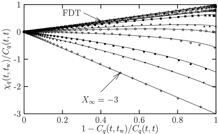
Figure 1: Normalized FD-plots for the FA model at $T=0.1$ in $d=3$ with fixed $t=2\times 10^{5}$ and running $t_{\mathrm{w}}\in[0,t]$. Symbols are results from simulations, full lines are the tree-level predictions. Wavevectors shown are $q=\pi/x$ with $x=1$, 2, 2.4, 3, 3.2, 4, 5.33, 6, 8, 12, and 16 (top to bottom). System size was $N=32^{3}$. Averages are over $4\times 10^{4}$ initial conditions.

The fluctuation-dissipation (FD) plots in Fig. 1 show that the tree-level calculations compare very well with numerical simulations of the FA model in $d=3$. We have also confirmed the diffusive scaling with $z=Dq^{2}t_{\mathrm{w}}$. Simulations were performed using a continuous time Monte Carlo algorithm. We measure $C_{q}(t,t_{\mathrm{w}})$ as the auto-correlation of the observable $A_{q}$, on a cubic lattice with periodic boundary conditions, $N=L^{3}$ and a linear size $L\gg\sqrt{Dt_{\mathrm{w}}}$. The susceptibility $\chi_{q}(t,t_{\mathrm{w}})$ is obtained by direct generalization of the “no-field” method of chatelain to continuous time. We show data using the prescription of Ref. mayer0 , plotting $\chi_{q}(t,t_{\mathrm{w}})/C_{q}(t,t)$ as a function of $1-C_{q}(t,t_{\mathrm{w}})/C_{q}(t,t)$ for fixed observation time, $t$, and varying waiting time, $0<t_{\mathrm{w}}\leq t$. The abscissa runs from 0 ($t_{\mathrm{w}}=t$) to $\approx$$1$ ($t_{\mathrm{w}}\ll t$). Using $t_{\mathrm{w}}$ as the running variable ensures that the slope of the plot is the FDR $X_{q}(t,t_{\mathrm{w}})$ MayBerGarSol . Other procedures, e.g. keeping $t_{\mathrm{w}}$ fixed, would give very different results Cri-Vio ; nicodemi ; newman ; kr ; buhot that could lead to erroneous conclusions.

In dimensions $d<d_{c}$ we need to take fluctuations into account. For $d=1$ exact scaling results can be derived for the FA model by considering a DLPC process with diffusion rate $D=c/2$. Because the long-time behavior of DLPC dynamics is diffusion controlled tauber we are free to choose the coalescence rate as $\lambda=D$ without affecting scaling results in the long-time regime ($t,t_{\mathrm{w}}\gg 1/c$) MaySol05 . We focus on the low temperature dynamics ($c\to 0$) and times $t\ll 1/\gamma\propto 1/c^{2}$ where branching can be neglected; the system is then still far from equilibrium as it ages.

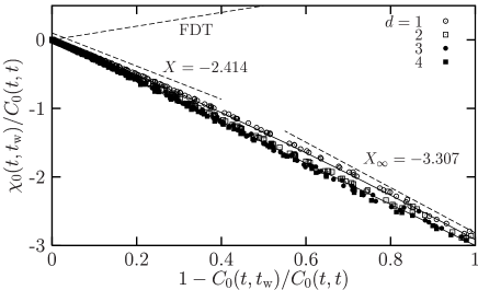
Figure 2: Normalized energy FD-plots for the FA model in dimensions $d=1$ to $4$, for fixed times $t$ and running waiting times $t_{\mathrm{w}}\in[0,t]$. Symbols show simulation data, for $T=0.2$ to 0.06 and $t=10^{4}$ to $10^{8}$. Full curves show a straight line with slope $X_{\infty}=-3$ and the exact limit plot in $d=1$ with asymptotic slopes shown as dashed lines.

To analyze our DLPC process we use the standard quantum mechanical formalism Kre95 : probabilities are mapped to states $|P(t)\rangle=\sum_{\boldsymbol{n}}p(\boldsymbol{n},t)|\boldsymbol{n}\rangle$, where $|\boldsymbol{n}\rangle=|n_{1},\ldots,n_{N}\rangle$, so that the master equation reads $\partial_{t}|P(t)\rangle=W_{C}|P(t)\rangle$, with $W_{C}$ the DLPC master operator. Correlations are then $\langle A(t)A(t_{\mathrm{w}})\rangle=\langle 1|A\mathrm{e}^{W_{C}\Delta t}A\mathrm{e}^{W_{C}t_{\mathrm{w}}}|P(0)\rangle$, where $\langle 1|=\sum_{\boldsymbol{n}}\langle\boldsymbol{n}|$ and $\Delta t\equiv t-t_{\mathrm{w}}$. DLPC dynamics is closely related to diffusion limited pair-annihilation (DLPA) Kre95 by a similarity transformation $B$: $W_{C}=BW_{A}B^{-1}$ where $W_{A}$ is the DLPA master operator with diffusion rate $D=c/2$ and annihilation rate $2\lambda=c$. Introducing empty and parity interval observables, $E_{\boldsymbol{i}}=\prod_{k=i_{1}}^{i_{2}-1}(1-n_{k})$ and $P_{\boldsymbol{i}}=\prod_{k=i_{1}}^{i_{2}-1}(1-2n_{k})$ respectively, where $\boldsymbol{i}=(i_{1},i_{2})$, one has $\langle 1|E_{\boldsymbol{i}}\mathrm{e}^{W_{C}\Delta t}=\langle 1|P_{\boldsymbol{i}}\mathrm{e}^{W_{A}\Delta t}B^{-1}$, $\langle 1|B=\langle 1|$ and $\langle 1|n_{i}B=2\langle 1|n_{i}$ Kre95 . If we interpret the $n_{i}$ in DLPA as domain walls in an Ising spin system, $n_{i}=\frac{1}{2}(1-\sigma_{i}\sigma_{i+1})$, then $P_{\boldsymbol{i}}\equiv\sigma_{i_{1}}\sigma_{i_{2}}$, and $W_{A}\equiv W_{\sigma}$ becomes the $T=0$ master operator for the Glauber-Ising spin chain. Substituting the two-spin propagator $\langle 1|\sigma_{i_{1}}\sigma_{i_{2}}\mathrm{e}^{W_{\sigma}c\Delta t}$ derived in MaySol04 and mapping back to DLPC then gives

$$\langle 1|E_{\boldsymbol{i}}\mathrm{e}^{W_{C}\Delta t}=H_{i_{2}-i_{1}}(2c\Delta t)\langle 1|+\sum_{j_{1}<j_{2}}G_{\boldsymbol{i},\boldsymbol{j}}^{(2)}(c\Delta t)\langle 1|E_{\boldsymbol{j}},$$ (4)

where $G_{\boldsymbol{i},\boldsymbol{j}}^{(2)}(\cdot)$ and $H_{n}(\cdot)$ are given in MaySol04 .

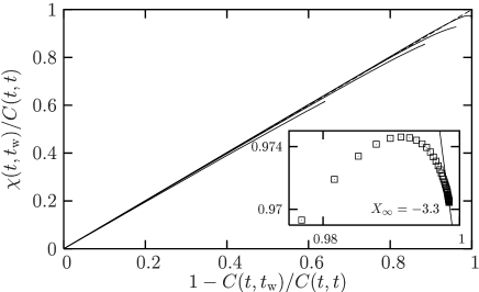
Figure 3: Normalized FD-plot for the local observable $n_{i}$ in the $d=1$ FA model at $T=0.1$ and $t=2\times 10^{4}$, $5\times 10^{4}$, $10^{5}$ and $10^{6}$ (bottom to top). The dashed diagonal is FDT. Inset: final part of the $t=10^{6}$ data, enlarged to show the non-monotonic response and $X_{\infty}\approx-3.307$ (full line).

Eq. (4) together with the identity $n_{i}=1-E_{(i,i+1)}$ is the key ingredient for the calculation of the two-time energy correlation and response functions $C_{0}(t,t_{\mathrm{w}}),R_{0}(t,t_{\mathrm{w}})$ in the $d=1$ FA model MaySol05 . Qualitatively a picture similar to $d>d_{c}$ emerges, but with the FDR now showing a weak dependence on the ratio $t/t_{\mathrm{w}}$. At equal times, $X_{0}(t/t_{\mathrm{w}}\to 1)=-(1+\sqrt{2})=-2.414\ldots$, while for $t/t_{\mathrm{w}}\to\infty$ the FDR approaches

$$X_{\infty}={3\pi}/({16-6\pi})=-3.307\ldots\quad(d=1).$$ (5)

Fig. 2 demonstrates complete agreement between our scaling predictions and simulation data in all dimensions. In $d=1$ the data fall on the curved limit FD-plot MaySol05 derived from (4). In dimensions $d=3,4$ the simulations are compatible with a constant FDR $X_{\infty}=-3$, Eq. (3). The data for $d=d_{c}=2$ suggest a slightly curved limit plot, possibly due to logarithmic corrections, but are still compatible with $X_{\infty}\approx-3$.

Numerically, the no-field method of chatelain becomes unreliable for small $q$. To get precise data as shown in Fig. 2 we used instead the exact relation

$$2R_{0}(t,t_{\mathrm{w}})=(1-2c)\partial_{t}n(t)+\partial_{t_{\mathrm{w}}}C_{0}(t,t_{\mathrm{w}})+C_{*}(t,t_{\mathrm{w}}).$$

for the energy-temperature response of a general class of kinetically constrained spin models MaySol05 . The quantity $C_{*}(t,t_{\mathrm{w}})$ is defined as $N^{-1}\langle H(t)U(t_{\mathrm{w}})\rangle_{\rm c}$, with $U=$ $\sum_{i}f_{i}(n_{i}-c)$ and $f_{i}\in\{0,1\}$ the kinetic constraint.

The auto-correlation $C(t,t_{\mathrm{w}})=\langle n_{i}(t)n_{i}(t_{\mathrm{w}})\rangle_{\rm c}$, and associated auto-response, $R(t,t_{\mathrm{w}})=T\delta\langle n_{i}(t)\rangle/\delta h_{i}(t_{\mathrm{w}})$, to a local perturbation $\delta H=-h_{i}n_{i}$, also have a negative FDR regime. Previous studies BuhGar02 ; buhot had suggested that the corresponding FD-plot has an equilibrium form, even during aging. A more careful analysis, however, reveals nonequilibrium contributions (Fig. 3). Exact long-time predictions for $C(t,t_{\mathrm{w}})$ and $R(t,t_{\mathrm{w}})$, and the resulting FDR, can be derived from (4) MaySol05 . One finds that, as for the energy, the FDR has the aging scaling $X(t/t_{\mathrm{w}})$. It crosses over from quasi-equilibrium behavior, $X\approx 1$, at $t/t_{\mathrm{w}}\approx 1$, to $X\approx X_{\infty}$ for $t/t_{\mathrm{w}}\gg 1$; notably, $X_{\infty}$ here is the same as for the energy, Eq. (5). However, the region in the FD-plot that reveals the nonequilibrium behavior shrinks as $O(1/\sqrt{t})$ as $t$ grows. This explains previous observations of pseudo-equilibrium and makes a numerical measurement of $X_{\infty}$ from the local observable $n_{i}$ very difficult. On the other hand, Fig. 2 shows that with the coherent counterpart, i.e. the energy, this would be straightforward, confirming a point made in MayBerGarSol . Numerical simulations for $d>1$ produce local FD-plots analogous to Fig. 3 but with $X_{\infty}=-3$. We emphasize that the non-monotonicity observed is not an artefact of using $t$ as the curve parameter, as in e.g. Cri-Vio ; kr .

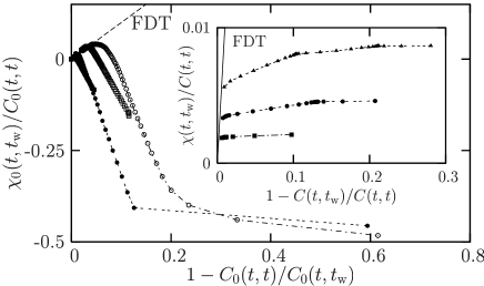
Figure 4: Normalized energy FD-plots for the East model for $(T,t)=(.15,100)$, $(.15,10^{5})$, $(.2,50)$ and $(.2,5000)$ (from left to right). Inset: Normalized FD-plot for local observables for $T=0.15$ and $t=10^{2}$, $10^{5}$ and $10^{7}$ (from bottom to top).

We have shown that some important components of the mean-field picture survive in systems with activated dynamics, in particular the concepts of time sectors (initial relaxation versus activated aging on long timescales) with associated well-defined FDRs. However, activation effects make these FDRs negative. This effect has not previously been observed in non-equilibrium critical dynamics, and calls into question whether effective temperature descriptions are possible for activated dynamics. Our arguments show that negative non-equilibrium responses should occur generically for observables whose relaxation couples to activation effects; activation need not be thermal, but can be via macroscopic driving, e.g. tapping of granular materials nicodemi ; DepSti . To illustrate how quantitative effects may vary, we consider briefly the East model RitSol03 of fragile glasses, leaving all details for a separate report. The behavior is richer due to the hierarchical nature of the relaxation, which leads to plateaux in the energy decay. Properly normalized energy FD-plots nevertheless have a simple structure, with three regimes (Fig. 4): for given $t$, equilibrium FDT is obeyed at small time differences $t-t_{\mathrm{w}}$, indicating quasi-equilibration within a plateau; a regime with a single negative FDR follows, coming from the activated relaxation process preceding the plateau at $t$; finally, the plot becomes horizontal, corresponding to all previous relaxation stages which decorrelate the system but do not contribute to the energy response. Interestingly, in the FD-plots for auto-correlation and auto-response (Fig. 4, inset), each relaxation stage of the hierarchy is associated with a well-defined effective temperature, a structure reminiscent of that found in mean-field spin glasses CugKur .

This work was supported by the Austrian Academy of Sciences and EPSRC grant 00800822 (PM); EPSRC grants GR/R83712/01, GR/S54074/01, and University of Nottingham grant FEF3024 (JPG).

References

- (1) Spin Glasses and Random Fields, edited by A.P. Young (World Scientific, Singapore, 1998).
- (2) L.F. Cugliandolo and J. Kurchan, Phys. Rev. Lett. 71, 173 (1993); J. Phys. A 27, 5749 (1994).
- (3) J. Kurchan and L. Laloux, J. Phys. A 29, 1929 (1996).
- (4) L. F. Cugliandolo, J. Kurchan, and L. Peliti, Phys. Rev. E 55, 3898 (1997).
- (5) S. Franz, M. Mézard, G. Parisi, and L. Peliti, Phys. Rev. Lett. 81, 1758 (1998).
- (6) D.S. Fisher and D.A. Huse, Phys. Rev. Lett. 56, 1601 (1986).
- (7) M.D. Ediger, Annu. Rev. Phys. Chem. 51, 99 (2000).
- (8) A. Crisanti and F. Ritort, J. Phys. A 36, R181 (2003).
- (9) A. Crisanti, F. Ritort, A. Rocco, and M. Sellitto, J. Chem. Phys. 113, 10615 (2000); P. Viot, J. Talbot, and G. Tarjus, Fractals 11, 185 (2003).
- (10) M. Nicodemi, Phys. Rev. Lett. 82, 3734 (1999).
- (11) J.P. Garrahan and M.E.J. Newman, Phys. Rev. E 62, 7670 (2000).
- (12) F. Krzakala, Phys. Rev. Lett. 94, 077204 (2005).
- (13) A. Buhot, J. Phys. A 36, 12367 (2003).
- (14) S. Fielding and P. Sollich, Phys. Rev. Lett. 88, 050603 (2002).
- (15) P. Mayer, L. Berthier, J.P. Garrahan, and P. Sollich, Phys. Rev. E 68, 016116 (2003); 70, 018102 (2004).
- (16) A. Buhot and J.P. Garrahan, Phys. Rev. Lett. 88, 225702 (2002).
- (17) A. Barrat and L. Berthier, Phys. Rev. Lett. 87, 087204 (2001).
- (18) H.E. Castillo, C. Chamon, L.F. Cugliandolo, and M.P. Kennett, Phys. Rev. Lett. 88, 237201 (2002).
- (19) L. Bellon, S. Ciliberto and C. Laroche, Europhys. Lett. 53, 511 (2001).
- (20) For a review see P. Calabrese and A. Gambassi, J. Phys. A 38, R133 (2005).
- (21) F. Ritort and P. Sollich, Adv. Phys. 52, 219 (2003).
- (22) G.H. Fredrickson and H.C. Andersen, Phys. Rev. Lett. 53, 1244 (1984).
- (23) S. Whitelam, L. Berthier, and J.P. Garrahan, Phys. Rev. Lett. 92, 185705 (2004); Phys. Rev. E 71, 026128 (2005).
- (24) M. Schulz and S. Trimper, J. Stat. Phys. 94, 173 (1999).
- (25) For a recent review see U.C. Täuber, M.Howard, and B.P. Vollmayr-Lee, J. Phys. A 38, R79 (1999).
- (26) B.P. Lee, J. Phys. A 27, 2633 (1994).
- (27) The form of the diffusion term arises because hopping is via creation of a defect at the arrival site. The hopping rate from site to depends only on the field at site .
- (28) C. Chatelain, J. Stat. Mech. P06006 (2004).
- (29) P. Sollich, S. Fielding, and P. Mayer, J. Phys. Condens. Matter 14, 1683 (2002).
- (30) P. Mayer and P. Sollich, unpublished.
- (31) K. Krebs, M.P. Pfannmüller, B. Wehefritz, H. Hinrichsen, J. Stat. Phys. 78, 1429 (1995).
- (32) P. Mayer and P. Sollich, J. Phys. A 37, 9 (2004).
- (33) M. Depken and R. Stinchcombe, Phys. Rev. E 71, 065102 (2005).