An algebraic approach to the study of weakly excited states for a condensate in a ring geometry

Abstract

We determine the low-energy spectrum and the eigenstates for a two-bosonic mode nonlinear model by applying the Inönü-Wigner contraction method to the Hamiltonian algebra. This model is known to well represent a Bose-Einstein condensate rotating in a thin torus endowed with two angular-momentum modes as well as a condensate in a double-well potential characterized by two space modes. We consider such a model in the presence of both an attractive and a repulsive boson interaction and investigate regimes corresponding to different values of the inter-mode tunneling parameter. We show that the results ensuing from our approach are in many cases extremely satisfactory. To this end we compare our results with the ground state obtained both numerically and within a standard semiclassical approximation based on su(2) coherent states.

PACS: 03.75.Fd, 03.65.Sq, 03.75Lm

1 Introduction

The dynamics of a bosonic fluid rotating within a thin torus and, particularly, the study of the properties relevant to its weakly-excited states have received recently a large attention [1]-[5] due to the rich phenomenology that characterizes such a system. For example, the quantization of fluid circulation is shown [3] to disappear whenever the physical parameters cause the hybridization of condensate ground state over different angular momentum (AM) states. A similar effect is found in the mean-field dynamics of the condensate wavefunction on a circle [4], where the circulation loses its quantized character when the system is in the soliton regime. The rotating fluid exhibits low-energy AM quantum states (corresponding to the presence of plateaus of quantized circulation) that determine the hybridization effect by a suitable tuning of the model interaction parameters [3]. In the simplest possible case, the model exhibits two momentum (bosonic) modes associated to two AM states (the ground-state and the first excited state) of the fluid. An almost identical model [6]-[13] has been studied thoroughly in the recent years within Bose-Einstein condensates (BEC) physics, where a condensate is distributed in two potential wells that exchange bosons via tunneling effect. The two-well model $H=U(n_{0}^{2}+n_{1}^{2})-\Delta(n_{0}-n_{1})/2-V_{0}(a_{0}a^{+}_{1}+a_{1}a^{+}_{0})$, where $a_{0}$, $a_{1}$ are bosonic space-modes and $n_{i}=a^{+}_{i}a_{i}$, displays hybridized states when the well-depth imbalance vanishes ($\Delta=0$).

For both models the energy regime of interest is that corresponding to the ground-state or to weakly excited states. In this respect, many authors have tried to develop approximation schemes able to provide a satisfactory analytical description of the low energy spectrum and of its states. The nonlinear character of the model Hamiltonian entails a difficult diagonalization process unless one resorts to numerical calculations. In this case the exact form of the spectrum is obtained quite easily. However, for N-well systems such as condensate arrays described by the Bose-Hubbard model, Josephson-junction arrays and, in general, N-mode bosonic systems [14], [15], the exact diagonalization requires a computational effort rapidly increasing with N. This motivates the interest in developing effective, analytical approximation methods able to solve the diagonalization problem.

The present work has been inspired by papers [2] and [3] where, among the variuos issues considered, the structure of the ground state of a ring condensate (within a two-AM-mode approximation of the bosonic quantum field) has been studied. As to the closely related two-well boson model, the same problem has been investigated in [16] within the hermitian phase operator method. In order to obtain a satisfactory description of the system ground state as well as of the weakly-excited states for the two-mode model, we implement, in the present paper, an algebraic approach based on the Inönü-Wigner contraction method [17]. This method allows one to simplify the algebraic structure of the Hamiltonian reducing the latter in a form apt to perform a completely analytic derivation of its spectrum. A well defined limiting procedure, mapping the original Hamiltonian generating algebra to a simpler algebra, often succeeds in reducing the nonlinear terms to a tractable form. These terms, originated by the boson-boson interaction and thus occurring in any model inherent in BEC dynamics, are known to make the Hamiltonian diagonalization a hard task. Such a technique and the effect of simplifying the algebraic structure of model Hamiltonians, has found a wide application in many fields of theoretical physics. It is well illustrated, e. g., in reference [18] where it is applied to study collective phenomena in nuclear models.

The contraction-method approach (CMA) –namely the contraction procedure and the ensuing approximation of weakly excited states– works well for the spectrum sectors where the energy levels are close to the minima and the maxima of the classical Hamiltonian and thus seems suitable for studying the low-energy regime of two-mode nonlinear models. The results obtained within the CMA in sections 2 and 3 will be compared both with the exact spectrum calculated numerically and with an alternative approch based on the coherent-state semiclassical appproximation (CSSA) reviewed in section 4.

We consider $N$ interacting bosons with mass $m$ whose boson-boson interaction can be either attractive or repulsive. These are confined in a narrow annulus whose thickness $2r$ is much smaller than the annulus radius $R$. Bosons are also acted by an external potential which causes inter-mode tunneling. Particularly, the rotating fluid with attractive interaction can be shown to be equivalent to the two-well model of repulsive bosons introduced previously. In the coordinate frame of the potential rotating with angular velocity $\omega$ and with $z$ axis parallel to total angular momentum $L_{tot}={L}_{z}$, the bosonic-field Hamiltonian reads

$${\hat{H}}_{bf}=\int d^{3}\,{\bf r}{\hat{\psi}}^{+}_{\bf r}\left[\frac{P^{2}}{2m}-\omega L_{z}+V_{ext}({\bf r})\right]{\hat{\psi}}_{\bf r}+\frac{1}{2}\int\!\!\int d^{3}{\bf r}\,d^{3}{\bf s}\,{\hat{\psi}}^{+}_{\bf r}\,{\hat{\psi}}^{+}_{\bf s}U(|{\bf r}-{\bf s}|){\hat{\psi}}_{\bf s}\,{\hat{\psi}}_{\bf r}$$

where ${\hat{\psi}}_{\bf r}=\hat{\psi}({\bf r})$ (${\hat{\psi}}^{+}_{\bf r}$) is the destruction (creation) boson field operator at ${\bf r}$. $V_{ext}$ is the confining potential. At low temperature, the interaction between dilute bosons is well represented by the Fermi contact interaction which entails the standard approximation $U(|{\bf r}-{\bf s}|)\simeq({4\pi\hbar^{2}a}/{m})\delta(|{\bf r}-{\bf s}|)$, where $a$ is the $s-$wave scattering length [2].

1.1 Two-mode approximation

The two-mode approximation involves only the first two states of AM, with eigenvalue equations $L_{z}\psi_{0}({\bf r})=0$ and $L_{z}\psi_{1}({\bf r})=\hbar\psi_{1}({\bf r})$. Field operator ${\hat{\psi}}({\bf r})$ in the two-mode basis of $L_{z}$ is thus written as ${\hat{\psi}}({\bf r})\simeq{a}_{0}\psi_{0}({\bf r})+{a}_{1}\psi_{1}({\bf r})$, where $a_{0}$, $a_{1}$ are bosonic operators and the validity of the two-mode approximation requires the condition $0<\omega<2\omega_{c}$ (greater angular velocities would involve other angular-momentum states). Within such an approximation [6, 9] and considering a thin torus ($r<<R$) ${\hat{H}}_{bf}$ reduces to [2] $H={g}(n^{2}_{0}+n^{2}_{1}-n_{0}-n_{1}+4n_{0}n_{1})/{2}-{\Delta}\hbar n_{1}/2-V_{0}(a_{1}^{+}a_{0}+a_{0}^{+}a_{1})$, where $n_{i}=a^{+}_{i}a_{i}$, $\Delta=2\hbar(\omega-\omega_{c})$, while $\omega_{c}=\hbar/(2mR^{2})$, $g=2\hbar^{2}a/(mR\pi r^{2})$, and $V_{0}$ are the critical angular frequency, the mean interaction energy per particle, and the asymmetry of potential $V_{ext}=V_{0}(e^{i\theta}+e^{i\theta})$, respectively. In the Schwinger picture [7] of algebra su(2) $H$ further simplifies becoming, up to a constant term,

$$H=-g\,J_{3}^{2}-2V_{0}J_{1}-\Delta J_{3}\,,$$ (1)

where $J_{3}=({n}_{1}-{n}_{0})/2$, $J_{1}=(J_{+}+J_{-})/2$, $J_{2}=(J_{+}-J_{-})/2i$ and $J_{+}=a^{+}_{1}a_{0}$ , $J_{-}=(J_{+})^{+}$. Such generators satisfy the commutators $[J_{r},J_{s}]=i\epsilon_{rsv}J_{v}$ ($\epsilon_{rsv}$ is the antisymmetric symbol) and commute with the total boson number operator ${n}_{1}+{n}_{0}$ ($n_{i}=a^{+}_{i}a_{i}$) whose eigenvalue $N$ is connected with the su(2)-representation index $J$ by $J=2N$. In such a scheme, the AM states are defined by

$$|J;m\rangle:=|n_{0}\rangle\otimes|n_{1}\rangle,\quad n_{1}=J+m,\,\,n_{0}=J-m,$$

where the $J_{3}$-basis states satisfy the eigenvalue equations $J_{3}|J;m\rangle=m|J;m\rangle$, and $J_{4}|J;m\rangle=J|J;m\rangle$, the index $J$ being the eigenvalue of $J_{4}=(n_{1}+n_{0})/2$. The positive (negative) sign of $g$ in model 1 implies that the effective interaction between bosons is repulsive (attractive). The conditions of weak asymmetry and interaction ensuring the validity of the model [2] are given by $|V_{0}|\ll\hbar\omega_{c}$, and $|g|\ll\hbar\omega_{c}$. The simple spin form of Hamiltonian 1 evidences how the attractive model ($g<0$) coincides with a (repulsive) two-site Bose-Hubbard Hamiltonian [7, 11] modeling two potential wells of different depth that share $N=2J$ bosons and exchange them via tunnel effect. The $N$-boson physical states can be written as $|\psi\rangle=\sum_{m=-J}^{J}X_{m}|J;m\rangle\,,$ while the Schrödinger equation $(i\hbar\partial_{t}-H)|\psi\rangle=0$ can be expressed in components as

$$i\hbar{\dot{X}}_{m}=\left(-gm^{2}-m\Delta\right)X_{m}-V_{0}\left[R^{J}_{m+1}X_{m+1}+R^{J}_{m}X_{m-1}\right],$$

once the symbol $R^{J}_{m}=[(J+m)(J-m+1)]^{1/2}$ has been defined. It worth noting that the study the algebraic structure characterizing the second-quantized Hamiltonian for a condensate trapped in two potential wells has received a large attention in the literature. In the seminal work [14] and in reference [15], in particular, such Hamiltonian has been shown to reduce, within a standard mean-field approach, to the sum of mode Hamiltonians describing the momentum conservation in the presence of inter-well boson exchange due to the tunneling. Each mode Hamiltonian is written in terms of operators $a_{k}$, $a_{-k}$ ($\pm k$ are the momentum modes) and can be reformulated as a linear combination of su(1,1) generators. In model 1 the momentum conservation is explicitly violated since one of the mode takes into account the fluid rotation. This fact entails that the previuos Schwinger realization of algebra su(2), rather than the algebra su(1,1) connected with the momentum conservation, characterizes the system.

In our analysis the dimensionless mean-value per boson of the angular momentum $\left<l_{z}\right>=\langle L_{z}\rangle/{\hbar N}$ (where the notation $\langle A\rangle=\langle\psi|A|\psi\rangle$ has been introduced) represents an important quantity. The angular momentum, in fact, expressed as

$$\left<l_{z}\right>=\sum_{m=-J}^{J}\frac{J+m}{2J}|X_{m}|^{2}=\left(\frac{1}{2}+\frac{\left<J_{3}\right>}{2J}\right),$$ (2)

relates the macroscopic behavior of the rotating condensate to the minimum-energy state properties through the ground-state components $X_{m}$. In the sequel we consider the spectral properties of model 1 both in the attractive case ($g<0$)

$$H_{a}=|g|\,J_{3}^{2}-2V_{0}J_{1}-\Delta J_{3},$$ (3)

and in the repulsive case ($g>0$)

$$H_{r}=-\left(|g|\,J_{3}^{2}+2V_{0}J_{1}+\Delta J_{3}\right).$$ (4)

It is worth noting that the study the ground-state properties of the repulsive case is closely related to the study the maximum-energy state for the attractive Hamiltonian. In fact, after the substitutions $V_{0}\rightarrow-V_{0}$ and $\Delta\rightarrow-\Delta$, the repulsive Hamiltonian is identical to the attractive one up to a factor $(-1)$. Since these two changes can be effected in a unitary way by means of transformations $e^{+i\pi J_{3}}J_{1}e^{-i\pi J_{3}}=-J_{1}$, and $e^{+i\pi J_{1}}J_{3}e^{-i\pi J_{1}}=-J_{3}$, respectively, the spectra of $H_{r}$ and $H_{a}$ turn out to satisfy the equation $spect[H_{a}(V_{0},\Delta)]$ $=-spect[H_{r}(-V_{0},-\Delta)]$. Concerning the parameter $\Delta$ of Hamiltonian 1, we note that the constraint $0\leq\omega\leq 2\omega_{c}$, implies the inequality $-2\hbar w_{c}<\Delta<2\hbar w_{c}$. The definition of the further parameters $\gamma={J|g|}/{2\hbar w_{c}}$, $\tau={V_{0}}/{J|g|}$, allows one to better characterize the regimes of the rotational dynamics as well as the conditions of validity of the present model. Parameter $\gamma$ (representing the ratio of the self-interaction energy per particle to the single-particle energy-level spacing) should satisfy the inequalities $2\gamma<<J$, $\tau<<{1}/{2\gamma}$, owing to the conditions $|g|<<\hbar\omega_{c}$ and $V_{0}<<\hbar\omega_{c}$, respectively. Both these conditions can be satisfied if $J=N/2$ is not excessively large [2]. Moreover, parameter $\tau={V_{0}}/(J|g|)$ allows one to distinguish, in both the attractive and repulsive case, three regimes:

• Fock regime, where $|g|\gg V_{0}J$ entails $\tau\ll{1}/{J^{2}}$,

• Josephson regime, where $V_{0}/J\ll|g|\ll V_{0}J$ entails ${1}/{J^{2}}\ll\tau\ll 1$,

• Rabi regime, where $|g|\ll V_{0}/J$ entails $\tau\gg 1$.

We note that the condition of weak asymmetry $|V_{0}|\ll\hbar\omega_{c}$ given by $\tau\ll{1}/{2\gamma}$ appears to be compatible with the first two regimes and with part of the Rabi regime.

2 The Inönü - Wigner contraction in the attractive case

We introduce a simple algebraic approach for studying the low-energy spectrum of Hamiltonians 3 and 4 for large $J$ whose essence consists in simplifying the nonlinearity due to the term $J^{2}_{3}$. The Inönü-Wigner contraction [19] supplies a method for mapping some given algebraic structure in a new one, as the result of a singular limiting process. The contraction is realized by defining a set of new operators $h_{i}$ as linear combinations $h_{i}=\sigma_{i}I+\Sigma_{k}c_{ik}g_{k}$ of the generators $g_{k}$ of a given algebra (identified by its commutators $[g_{r},g_{s}]=\varepsilon_{rsk}g_{k}$) and of the identity operator $I$. Selecting an appropriate parametrization $c_{ik}(x)$ of the linear-map coefficients, the contraction enacted by means of the limit $x\to 0$ is able to generate the new algebraic structure $[h_{i},h_{j}]=e_{ijk}h_{k}$ whose structure constants $\{e_{ijk}\}$ differ from the original ones $\{\varepsilon_{rsk}\}$. For the algebra su(2) the contraction of the algebra mapping is driven by $x=1/\sqrt{J}$ (with $J\rightarrow\infty$) and generates, in this limit, the harmonic oscillator (namely the Heseinberg-Weyl) algebra [20].

The classical study of attractive ($g<0$) Hamiltonian $H_{a}=|g|\,J_{3}^{2}-2V_{0}J_{1}-\Delta J_{3}$ developed in A demonstrates (see formula 35) how $J_{1}\simeq+J$, $J\gg|J_{2}|,|J_{3}|\simeq 0$, at low energies. This suggests the correct way to implement the contraction scheme. In the present attractive case we can build the following transformation

$$h_{1}=J_{1}-{I}/{x^{2}},\,\,h_{2}=xJ_{2},\,\,h_{3}=xJ_{3},$$ (5)

where $J_{4}=J\,I$. The Inönü-Wigner contraction is realized when such a $x$-dependent transformation is considered in the (singular) limit $J=1/x^{2}\rightarrow\infty$. In this case the objects $\{J_{i}\}$ (with $i=1,2,3,4$), defining algebra $u(2)$, transform into the new objects $\{h_{i},I\}$ (with $i=1,2,3$) that satisfy the following commutation relations:

$$[h_{2},h_{3}]=i(x^{2}h_{1}+I)\to iI,\,\,[h_{1},h_{2}]=x[J_{1},J_{2}]=ih_{3}\,,$$ (6)

$$[h_{1},h_{3}]=x[J_{1},J_{3}]=-ih_{2}\,,\,\,[h_{i}\,,\,I\,]=0\,.$$ (7)

In the limit $x={1}/{\sqrt{J}}\to 0$, the latter reproduce the commutation relations of Weyl-Heisemberg algebra: $[q,p]=i$, $[n,q]=-ip$, $[n,p]=iq$, $n=(q^{2}+p^{2})/2$, thereby suggesting the identifications $h_{1}\equiv-n$, $h_{2}\equiv-p$, $h_{3}\equiv q$. By combining the latter with definitions 5 we find that the contraction gives $J_{1}\rightarrow J-n$, $J_{2}\rightarrow-\sqrt{J}p$, $J_{3}\rightarrow\sqrt{J}q$. Correspondingly, Hamiltonian $H_{a}$ becomes $H_{a}=|g|Jq^{2}+2V_{0}n-2V_{0}J-\Delta\sqrt{J}q$, which, by defining $\Omega=[1+{1}/{\tau}]^{1/2}$, and $Q=q-\chi$ with $\chi={\sqrt{J}\Delta}/{2V_{0}\Omega^{2}}$, and $\tau=V_{0}/J|g|$, reduces to the form

$$H_{a}=V_{0}\left[{p^{2}}+\Omega^{2}Q^{2}-2J-\frac{J\Delta^{2}}{4V_{0}^{2}\Omega^{2}}\right]\,.$$ (8)

Since ${p^{2}}+\Omega^{2}Q^{2}=2\Omega(n+1/2)$ is diagonalized by the harmonic-oscillator eigenstates $\Psi_{n}(Q)=\langle Q|E_{n}\rangle=N_{n}e^{-\Omega Q^{2}/{2}}H_{n}\left({\sqrt{\Omega}Q}\right)$, the eigenvalues of Hamiltonian 8 are found to be

$$E_{n}=V_{0}\left[2\Omega(n+1/2)-2J-\frac{J\Delta^{2}}{4\Omega^{2}V^{2}_{0}}\right]\,.$$ (9)

The corresponding eigenvalue equation $H_{a}|E_{n}\rangle=E_{n}|E_{n}\rangle$ in the $J_{3}$ basis, where $|E_{n}\rangle=\Sigma_{m}X_{n}(m)|J,m\rangle$, can be written as $\Sigma_{m}(H_{a})_{\ell m}X_{n}(m)=E_{n}X_{n}(\ell)$ with $(H_{a})_{\ell m}=\langle J,\ell|H_{a}|J,m\rangle$. In the limit $J>>1$, equation $J_{3}|J,m\rangle=m|J,m\rangle$ is replaced by $q|J,m\rangle=(m/{\sqrt{J}})|J,m\rangle$. Therefore the eigenvalue $m/\sqrt{J}$ can be seen as a continuous variable which naturally identifies with the variable $q\simeq J_{3}/\sqrt{J}$ used within the approximation scheme just discussed. The component version of the eigenvalue equation for $H_{a}$ then reduces (see reference [20] for details) to the equation $H_{a}(Q,p)\Psi_{n}(Q)=E_{n}\Psi_{n}(Q)$ solved above. Components $X_{m}(E_{n})$ thus appear to be given by $X_{m}(E_{n})=\Psi_{n}(Q)$ that entail the explicit expression for the eigenstates

$$|E_{n}\rangle=\Sigma_{m}X_{m}(E_{n})|J;m\rangle,\quad X_{m}(E_{n})=N_{n}H_{n}({\sqrt{\Omega}Q})e^{-{\Omega Q^{2}}/{2}}$$ (10)

with $Q={m}/{\sqrt{J}}-\chi$. The normalization constants $N_{n}$ are determined through the condition $\langle E_{n}|E_{n}\rangle=1$ implying that

$$\!1=\sum^{J}_{m=-J}X^{2}_{m}(E_{n})\simeq\int^{\infty}_{-\infty}dq\frac{N^{2}_{n}}{\sqrt{J}}\,H^{2}_{n}\left[{\sqrt{\Omega}}(q-\chi)\right]\,e^{-\Omega(q-\chi)^{2}}\,,$$ (11)

where $\pm J$ has been replaced with $\pm\infty$. Such an approximation is acceptable until the condition

$$|\chi|<{\sqrt{J}}-\sqrt{2n/\Omega}$$ (12)

–evinced from the interval containing the Hermite-polynomial zeros– is fulfilled. Excluding the case $\tau\gg 1$, this condition is always valid provided $n<<J$. Thus constants $N_{n}$ are given by $N_{n}=[(J\Omega)^{1/2}/(\pi^{1/2}2^{n}n!)]^{1/2}$.

Another important check concerns the possibility of considering $m/\sqrt{J}$ as a continuous variable. The characteristic scale is established by the gaussian deviation $\sqrt{2/\Omega}$ which must be compared with the smallest variation $1/\sqrt{J}$ of $q$. The resulting condition $1/\sqrt{J}<\sqrt{2/\Omega}$ can be written as

$$1<\frac{2J}{\Omega}=2J\left[\frac{V_{0}}{V_{0}+J|g|}\right]^{1/2}=2J\left[\frac{\tau}{\tau+1}\right]^{1/2}.$$

While in the Rabi and Josephson regimes ($1/J^{2}<<\tau$) the latter is fully satisfied, in the Fock regime, where $\tau<<1/J^{2}$, such condition is violated. We notice that for $\tau\simeq 1/J^{2}$ (namely $|g|\approx JV_{0}$) a unique component $X_{m}$ appears to contribute to states $|E_{n}\rangle$ since the gaussian amplitude becomes very small. For example, in the case of the ground-state one has

$$|E_{0}\rangle=\Sigma_{m}N_{0}e^{-\frac{\Omega}{2}\left(\frac{m}{{\sqrt{J}}}-\chi\right)^{2}}|J,m\rangle\simeq N_{0}e^{-\frac{\Omega}{2}\left(\frac{m_{*}}{{\sqrt{J}}}-\chi\right)^{2}}|J,m_{*}\rangle\,,$$ (13)

where $m_{*}$ is the integer closest to ${\sqrt{J}}\chi\simeq\Delta/2|g|$. Nevertheless, in the special case when $\Delta/2|g|=m_{*}+1/2$, the two states $|J,m_{*}\rangle$ and $|J,m_{*}+1\rangle$ equally contribute to $|E_{0}\rangle$ which is given by

$$|E_{0}\rangle\simeq N_{0}e^{-\frac{\Omega}{8J}}(|J,m_{*}\rangle+|J,m_{*}+1\rangle).$$ (14)

To summarize, we note how the ground-state $|E_{0}\rangle$ is essentially formed by a unique component corresponding to $|J,m_{*}\rangle$ in the whole parameter range $m_{*}-1/2<\Delta/2|g|<m_{*}+1/2$. The resonance of the system between two equivalent states crops up whenever $\Delta/|g|$ assumes integer values given by $\Delta/|g|\equiv 2m+1$ with $-J\leq m\leq J$. Such condition can be implemented by varying $\Delta$ with $|g|=const$ thus leaving $\Omega$ unchanged.

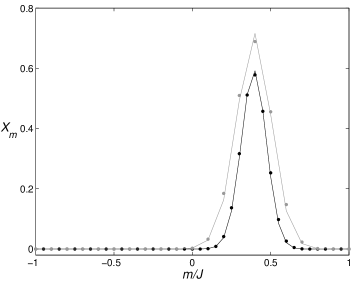
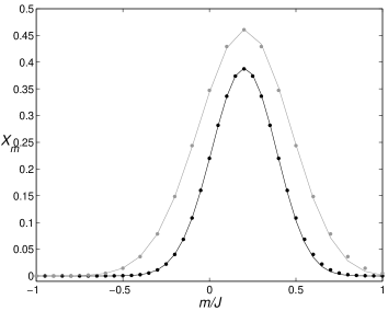
Figure 1: In both panels, grey (dark) diamonds describe the ground-state components $X_{m}$, obtained from formula 10, for $N=20$ ($N=40$) within the contraction-method approach (CMA). The edges of the grey/dark piecewise linear curves represent components $X_{m}$’s calculated numerically. Left panel: Josephson regime in the attractive case with $\tau=0.02$, $\nu=0.8$. CMA components $X_{m}$’s and $X_{m}$’s calculated numerically are almost indistinguishable. Right panel: Attractive case with $\tau=1.0$ (transition point from Josephson to Rabi regime) and $\nu=0.8$. No difference is visible between CMA $X_{m}$’s and $X_{m}$’s calculated numerically.

2.1 Comparison of different regimes

For $\tau>1/J^{2}$ (Rabi and Josephson regimes), one easily calculates the dimensionless mean AM per boson $\langle l_{z}\rangle$ based on state $|E_{0}\rangle$, as given by formula 10, and exploiting the normalization integral 11. Recalling that $\langle J_{3}\rangle=\sum^{J}_{m=-J}mX^{2}_{m}(E_{0})$, one finds

$$\!\!\langle l_{z}\rangle=\frac{1}{2}\left(1+\frac{\langle J_{3}\rangle}{J}\right)\simeq\frac{1}{2}+\frac{\tau\Delta}{4V_{0}(1+\tau)}\,,\,\,\,\langle J_{3}\rangle\simeq{\sqrt{J}}\chi=\frac{{J}\tau\Delta}{2V_{0}(1+\tau)},$$ (15)

where $\langle J_{3}\rangle$ matches exactly formula 36 obtained in the classical study of the attractive model. This result cannot be used in the Fock regime where the ground state has, at most, either one or two dominating components. In the other two regimes, the second of equations 15 entails the further consistence condition

$$-1\leq\langle J_{3}\rangle/J={\tau\Delta}/{[2V_{0}(1+\tau)]}\leq+1\,,$$ (16)

which has to be verified in each regime. In view of the condition $|\langle J_{3}\rangle|<<J$ required to implement the contraction procedure, formula 16 should be imposed in the stronger version $|\tau\Delta/[2V_{0}(1+\tau)]|<<1$. However, the numerical (exact) determination of the ground state for various choices of parameters reveals that our approximate procedure works well also in the case when $|\tau\Delta/[2V_{0}(1+\tau)]|$ is not particularly small.

Fock regime. The main feature of this case ($\tau\ll{1}/{J^{2}}$) is that the mean dimensionless AM per boson is a step function of $\Delta$ (as to this well-known effect see, e. g., reference [3]). If one simplifies the form of states 13 and 14 by setting $|E_{0}\rangle=|J,m\rangle$ and $|E_{0}\rangle=(|J,m\rangle+|J,m+1\rangle)/\sqrt{2}$ in correspondence to the appropriate values of $\Delta$, the dimensionless mean AM per boson is found to be

$$\langle l_{z}\rangle=\frac{1}{2}+\frac{m}{2J},\quad\langle l_{z}\rangle=\frac{1}{2}+\frac{m}{2J}\pm\frac{1}{4J},$$

for $m-1/2<\Delta/2|g|<m+1/2$ and $\Delta/2|g|=m\pm 1/2$, respectively, corresponding to the two choices of the Fock ground state $|E_{0}\rangle$. This illustrates the AM step character (related to the Hess-Fairbank effect) as well as its ”singular” behavior when $\Delta/2|g|=m\pm 1/2$. Notice that considering the simplified form for $|E_{0}\rangle$ is equivalent to assume the net predominance of one or two components. The results just found are consistent with the limit $\tau\to 0$, where $H_{a}=|g|J_{3}^{2}-\Delta J_{3}$ can be diagonalized in a direct way.

Josephson and Rabi regimes. In these cases $1/J^{2}<<\tau<<1$ and $1<<\tau$, respectively. Based on the above formulas, one finds $\langle J_{3}\rangle\simeq{{J}\tau\Delta}/{2V_{0}}$ (Josephson case) and $\langle J_{3}\rangle\simeq{J\Delta}/{2V_{0}}$ (Rabi case) giving the mean dimensionless AM per boson

$$\langle l_{z}\rangle=\frac{1}{2}\left[1+\frac{\tau\Delta}{2V_{0}}\right]\,,\quad\langle l_{z}\rangle=\frac{1}{2}\left[1+\frac{\Delta}{2V_{0}}\right]\,,$$

respectively. Owing to formulas 15 and 16, in the Josephson case, the range of parameter $\Delta$ is $[-2J|g|,\,\leq 2J|g|]$. For this regime, the further condition 12 reduces to $(2n\tau^{1/2}/J)^{1/2}+(\Delta/2J|g|)<1$. In the Rabi case, condition 16 on $\langle J_{3}\rangle$ entails that $\Delta$ ranges in $[-2J\tau|g|,\,2J\tau|g|]$ ($2J\tau|g|=2V_{0}$) which is, in principle, much larger than the range allowed in the Josephson case. Considering once more condition 12, this gives in the Rabi case $(2n\tau^{1/2}/J)^{1/2}+(\Delta/2V_{0})<1$. On easily checks that weakly excited states $|E_{n}\rangle$ satisfy the conditions on the restricted range of $\Delta$ provided $n<<J$, and $|\Delta|<<2J|g|$, $|\Delta|<<2V_{0}$ in the Josephson case and in the Rabi case, respectively. In both cases the latter inequalities represent condition 16 in its stronger version.

3 The Inönü - Wigner contraction in the repulsive case

The classical study of repulsive Hamiltonian $H_{r}=-(|g|\,J_{3}^{2}+2V_{0}J_{1}+\Delta J_{3})$, discussed in A, shows that, with $\tau=V_{0}/J|g|>1$ (Rabi regime), the energy minimum is such that $J_{1}=J$, $J_{2}=J_{3}=0$. As shown by equation 38, a generic state near the minumun is such that $J_{1}\simeq J$, $|J_{2}|$, $|J_{3}|\ll J$. In the Fock/Josephson regimes, where $\tau=V_{0}/J|g|<1$, Hamiltonian $H_{r}$ displays two minimum-energy states (see equation 40) entailing low-energy configurations characterized by $J_{3}\simeq\pm J$, $|J_{2}|$, $|J_{1}|\ll J$.

3.1 Repulsive regime with $\tau>1$

In the Rabi regime ($\tau>1$), the CPA valid for the attractive model can be implemented again. Then assuming $h_{1}$, $h_{2}$, $h_{3}$ as in formulas 5 the result of the contraction gives $J_{1}\rightarrow J-n$, $J_{2}\rightarrow-\sqrt{J}p$, and $J_{3}\rightarrow\sqrt{J}q$, which reduce $H_{r}$ to a quadratic form. By defining $Q=q-c$, with $c={\sqrt{J}}\Delta/(2V_{0}W^{2})$, the final form of $H_{a}$ is found to be

$$H_{a}=V_{0}\left[p^{2}+W^{2}Q^{2}-2J-\frac{{J}\Delta^{2}}{4V^{2}_{0}W^{2}}\right].$$ (17)

Since the eigenvalues of $p^{2}+W^{2}q^{2}$ are $\Lambda_{n}=2W(n+1/2)$, the spectrum of $H_{r}$ is

$$E_{n}=V_{0}\left[2W(n+1/2)-2J-\frac{{J}\Delta^{2}}{4V^{2}_{0}W^{2}}\right].$$ (18)

As in the attractive case, the eigenfunctions $\Phi_{n}(Q)$ of Hamiltonian 17 allow one to determine components $X_{m}$ through the formula $X_{m}(E_{n})=\Phi_{n}(Q)$. The energy eigenstates turn out to be

$$|E_{n}\rangle=\Sigma_{m}X_{m}(E_{n})|J;m\rangle\,,\quad X_{m}(E_{n})=N_{n}H_{n}({\sqrt{W}}Q)e^{-\frac{WQ^{2}}{2}},$$ (19)

with $Q={m}/{\sqrt{J}}-c$. This description is valid if the conditions on the gaussian deviation and the Hermite-polynomyal zeros ${1}/{\sqrt{J}}<\sqrt{{2}/{W}}$ and $|c|<{\sqrt{J}}-{\sqrt{{2n}/{W}}}$, respectively, which can be rewritten as $1<2J\tau/(\tau-1)$ and $|\Delta|\tau/[2V_{0}(\tau-1)]<1-\{2n\tau^{1/2}/[J(\tau-1)^{1/2}]\}^{1/2}$, are satisfied. For $\tau\gg 1$, the first condition is fulfilled, while the second one gives ${\Delta}/{2V_{0}}<1-\sqrt{2n/J}$. The latter is satisfied if ${\Delta}/{2V_{0}}<1$. Weakly excited states $|E_{n}\rangle$ with $n>0$ can be also considered provided $J\gg 2n$. Under such conditions, the mean dimensionless AM per boson is a linear function of $\Delta$

$$\left<l_{z}\right>=\frac{1}{2}(1+\langle J_{3}\rangle/J)=\frac{1}{2}\left[1+\frac{\Delta\tau}{2V_{0}(\tau-1)}\right]\,,\quad\langle J_{3}\rangle=c\sqrt{J}={J\Delta\tau}/{2V_{0}(\tau-1)}\,,$$

giving $\left<l_{z}\right>\simeq(1+{\Delta}/{2V_{0}})/2$ for $\tau>>1$. Notice that $\langle J_{3}\rangle$ coincides with formula 39 for the minimum of the classical repulsive model and that, in the Rabi regime, $\left<l_{z}\right>$ has the same form both for attractive bosons ($g<0$) and for repulsive bosons ($g>0$).

3.2 Repulsive case with $\tau<1$

In this case, the classical ground-state configuration corresponds to two minima. The contraction scheme can be implemented in two ways by assuming $h_{2}=xJ_{2}$, $h_{1}=xJ_{1}$, and $h_{3}=J_{3}\mp{I}/{x^{2}}$ which entails $[h_{1},h_{2}]=\pm ix^{2}h_{3}$, $[h_{2},h_{3}]=ih_{1}$, and $[h_{3},h_{1}]=ih_{1}$. Notice that $h_{3}=J_{3}\mp{I}/{x^{2}}$ allows to describe the two classical minima by further selecting a suitable definition for $h_{3}$. The result of the contractions demonstrates the two possible choices

$$h_{3}=-n,\,h_{2}=J_{2}/\sqrt{J}\rightarrow p,\,h_{1}=J_{1}/\sqrt{J}\rightarrow q,$$ (20)

and

$$h_{3}=+n,\,h_{2}=J_{2}/\sqrt{J}\rightarrow-p,\,h_{1}=J_{1}/\sqrt{J}\rightarrow q,$$ (21)

that are naturally associated to the $J_{3}$-positive and $J_{3}$-negative minimum, respectively. The repulsive Hamiltonian $H_{r}=-(|g|\,J_{3}^{2}+2V_{0}J_{1}+\Delta J_{3})$ thus can be cast in the two (local) forms

$$H_{r}=-|g|\Bigl{[}J^{2}-2J\,n+2\tau J^{3/2}q+\frac{s\Delta}{|g|}(J-n)\Bigr{]},$$ (22)

where $s=\pm$ recalls the presence of two minima. Notice that $H_{r}$ could be diagonalized by means of the procedure used in the attractive case, provided one adopts the rotated basis $\{|m\rangle_{1}=\exp(-i\pi J_{2}/2)|m\rangle\}$ of $J_{1}$ and regards the $q$ eigenvalues $m/\sqrt{J}$ as a continuous index. Unfortunately, while the evaluation of the energy eigenvalues is very easy in the ”rotated” $J_{1}$ basis $\{|m\rangle_{1}=\exp(-i\pi J_{2}/2)|m\rangle,|m|\leq J\}$, the eigenstates must be counter-rotated to recover the $J_{3}$-basis representation that we have adopted in the other cases/regimes. This is a difficult problem in that recovering the eigenstates description in the $J_{3}$ basis requires that the transformation matrix element $\langle m^{\prime}|\exp(-i\pi J_{2}/2)|m\rangle$ is calculated explicitly and is formulated in the limit where $m/\sqrt{J}$ is a continuous index.

To skip this problem, we observe that, owing to formulas 20 and 21 derived by the contraction procedure, $J^{2}_{3}+J^{2}_{2}+J^{2}_{1}=J(J+1)\simeq J^{2}$ can be rewritten as $J^{2}_{3}\simeq 2Jn-J^{2}$ while $J_{3}=\pm(J-n)$. We thus obtain the linearized expression $J^{2}_{3}\simeq-J^{2}\pm 2JJ_{3}$. Hamiltonian 22 reduces to $H_{r}=-|g|\bigl{[}-J^{2}\pm 2JJ_{3}+2\tau JJ_{1}+({\Delta}/{|g|})J_{3}\bigr{]}$, whose digonalization is rather simple owing to the linear dependence on su(2) generators. Rewriting the latter as $H^{\pm}_{r}=|g|\Bigl{[}J^{2}\mp(2J\pm\delta)J_{3}-2\tau JJ_{1}\Bigr{]}$ where $\delta=\Delta/|g|$, the unitary transformations $U_{\pm}=\exp(\mp iJ_{2}\phi_{\pm})$ entail

$$H^{\pm}_{r}=|g|\Bigl{[}J^{2}\mp R_{\pm}\,U_{\pm}J_{3}U^{+}_{\pm}\Bigr{]}\,,$$ (23)

with $R_{\pm}=\sqrt{(2J\pm\delta)^{2}+4\tau^{2}J^{2}}$. The action of $U_{\pm}$ is given by

$$U_{-}J_{3}U^{\dagger}_{-}=J_{3}\cos\phi_{-}-J_{1}\sin\phi_{-}\,,\quad U_{+}J_{3}U^{\dagger}_{+}=J_{3}\cos\phi_{+}+J_{1}\sin\phi_{+}\,,\quad$$ (24)

where angles $\phi_{\pm}$ are definded by ${\rm tg}\phi_{-}={2\tau J}/{(2J-\delta)}$, ${\rm tg}\phi_{+}={2\tau J}/{(2J+\delta)}$. The energy spectrum is thus represented by the eigenstates and the eigenvalues

$$|E^{\pm}_{m}\rangle=U_{\pm}\,|m\rangle,\quad E^{\pm}_{m}=|g|\Bigl{[}J^{2}\mp m\sqrt{(2J\pm\delta)^{2}+4\tau^{2}J^{2}}\Bigr{]},$$ (25)

respectively. One should recall that, within the present approximation scheme, these eigenvalues are significant for $|m|\approx J$. Moreover, we notice that $U_{\pm}\to\bf 1$ for $\tau\to 0$ thus reproducing the correct spectrum of the uncoupled model. The eigenvalues corresponding to the energy minima are obtained by setting $m=-J$ and $m=+J$ for $H^{-}_{r}$ and $H^{+}_{r}$, respectively, and read

$$E^{\pm}_{M}(\delta):=E^{\pm}_{\pm J}=|g|\Bigl{[}J^{2}-J\sqrt{(2J\pm\delta)^{2}+4\tau^{2}}\,\Bigr{]}.$$ (26)

The choice of the signs $\pm$, and thus the recognition of the lowest-energy states, is related to the sign of $\delta$. This is discussed below.

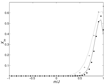
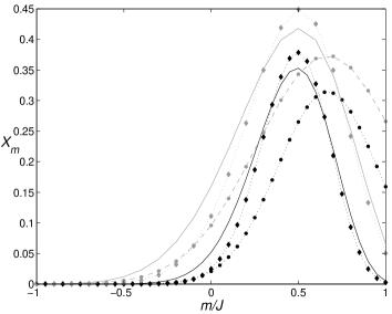
Figure 2: Both panels concern the repulsive case. Grey (dark) squares, diamonds, points and (piecewise-linear, continuous, dotted or dashed) curves are relevant to $N=20$ ($N=40$). Left panel: $\tau=0.6$ (Josephson regime), $\nu=0.8$. Within the CMA, the ground-state components $X_{m}$’s, given by formula 29 and described by squares, well approximate the $X_{m}$’s (edges of the grey/dark piecewise-linear curves) calculated numerically. Right panel: $\tau=1.6$ (Rabi regime), $\nu=0.8$. Points (diamonds) –joined by dashed/dotted lines to better distiguish different cases– describe ground-state $X_{m}$’s within the CMA (CSSA) referred to formula 19 (formula 33). Continuous piecewise-linear curves represent $X_{m}$’s obtained numerically. The CSSA is qualitatively better than the CMA approximation where curves are shifted on the right. Further comments are given in section 5.

The states associated with eigenvalues 26 take the form of su(2) coherent states [22]. The standard su(2) picture of such states, also known as Bloch states, is given by

$$|{-\,J},\xi\rangle=e^{\xi J_{+}-\xi^{*}J_{-}}|-\!J\rangle=\sum^{2J}_{s=0}\frac{C_{Js}z^{s}|s-J\rangle}{(1+|z|^{2})^{J}}$$ (27)

with $C_{Js}=\sqrt{(2J)!/s!(2J-s)!}$, while the coherent-state labels $z=|z|e^{i\theta}$ and $\xi=|\xi|e^{i\theta}$ are such that $|z|={\rm tg}|\xi|$, $z\in\bf C$. Since the minimum-energy states have the form

$$|E^{\pm}_{M}\rangle=e^{\mp iJ_{2}\phi_{\pm}}\,|\pm J\rangle,$$ (28)

where $\mp iJ_{2}\phi_{\pm}=\mp(\phi_{\pm}/2)(J_{+}-J_{-})$, the link with the coherent-state picture is almost immediate. Upon setting $\xi=\mp\phi_{\pm}/2$, the corresponding $z$ reads $z=\mp{\rm tg}(\phi_{\pm}/2)=\mp{2\tau J}/({2J\pm\delta})$. In view of this, eigenstate $|E^{-}_{M}\rangle$ takes the new form

$$|E^{-}_{M}\rangle=\cos^{2J}(\phi_{-}/2)\sum^{2J}_{s=0}C_{Js}{\rm tg}^{s}(\phi_{-}/2)|s-J\rangle.$$ (29)

If $\delta<0$, state $|E^{-}_{M}(\delta)\rangle$ (we make explicit the dependence from $\delta$ to illustrate clearly the difference between the absolute minumum and the local minimum) corresponds to the lowest-energy state with eigenvalue $E^{-}_{M}(\delta)=|g|[\,J^{2}-J\sqrt{(2J+|\delta|)^{2}+4\tau^{2}}\,]$, since $E^{-}_{M}(\delta)<E^{+}_{M}(\delta)$ (see equation 26). The remaining state $|E^{+}_{M}(\delta)\rangle$ represents the local minimum found in the classical dynamics. In the opposite case $\delta>0$, the lowest energy state identifies with $|E^{+}_{M}\rangle$. This in fact corresponds to (see equation 26) $E^{+}_{M}(\delta)=|g|[\,J^{2}-J\sqrt{(2J+\delta)^{2}+4\tau^{2}}\,]$, which satisfies $E^{+}_{M}(\delta)<E^{-}_{M}(\delta)$ for $\delta>0$. Notice that $E^{-}_{M}(-|\delta|)\equiv E^{+}_{M}(\delta)$. This feature is important because it confirms the symmetry property $e^{+i\pi J_{1}}H_{r}(\delta)\,e^{-i\pi J_{1}}$ $=H_{r}(-\delta)$ of repulsive Hamiltonian $H_{r}(\delta)=-|g|(J_{3}^{2}+2J\tau J_{1}+\delta J_{3})$ stating that the spectra of the cases $\delta>0$ and $\delta<0$ must coincide, the relevant Hamiltonians being related by a unitary transformation. Based on this fact, we find as well $|E^{+}_{M}(\delta)\rangle=e^{+i\pi J_{1}}|E^{-}_{M}(-|\delta|)\rangle$. By acting with $e^{i\pi J_{1}}$ on $|E^{-}_{G}(-|\delta|)\rangle$ we get the expression

$$|E^{+}_{M}(\delta)\rangle=e^{-iJ_{2}\phi_{-}}e^{+i\pi J_{1}}\,|-\!J\rangle=e^{iJ\pi}e^{-iJ_{2}\phi_{-}}|+\!J\rangle$$ (30)

[notice that $\phi_{-}=\phi_{-}(-|\delta|)$], where we have used the property of the $J_{3}$-basis states $e^{iJ_{1}\pi}|m\rangle=e^{iJ\pi}|-m\rangle$. Upon observing that $\phi_{-}(-|\delta|)=\phi_{+}(+|\delta|)$ we conclude that the unitary transformation reproduces, up to a phase factor, the diagonalization-process formula $|E^{+}_{M}\rangle=e^{-iJ_{2}\phi_{+}}\,|+\!J\rangle$ in a consistent way.

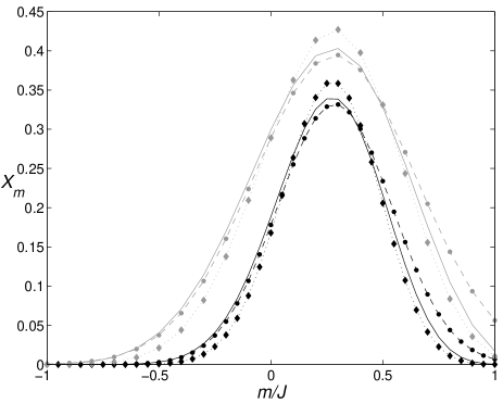
Figure 3: Repulsive case, $\tau=2.4$ (Rabi regime), $\nu=0.8$. Grey (dark) diamonds, points and piecewise-linear curves are relevant to $N=20$ ($N=40$). Diamonds (points) –joined by dashed/dotted lines to better distiguish different cases– describe ground-state $X_{m}$’s given by formula 19 (formula 33) within the CMA (CSSA). Piecewise-linear curves have the usual meaning. Both CSSA and CMA are satisfactory. Further comments are given in section 5.

Therefore, the ground state of the case $\delta>0$ is obtained by calculating formula 30 explicitly, which gives

$$|E^{+}_{M}\rangle=\cos^{2J}\left({\phi_{+}}/{2}\right)\,\sum^{2J}_{s=0}{C_{Js}{\rm tg}^{s}\left({\phi_{+}}/{2}\right)\,|J-s\rangle},$$ (31)

where $\phi_{+}(+|\delta|)=\phi_{-}(-|\delta|)$. We notice that $|E^{+}_{M}\rangle$ corresponds to a coherent state $|+\!J,\xi\rangle=e^{\xi J_{+}-\xi^{*}J_{-}}|+\!J\rangle$ whose extremal state is $|J\rangle$ (instead of $|-J\rangle$) where $|v|=tg|\xi|$ with $v=-tg(\phi_{-}/2)$ reproduces 31. As in the case $\delta<0$, the remaining state $|E^{-}_{M}(\delta)\rangle$ describes the quantum counterpart of the local minimum. The expectation value of $J_{3}$ is easily carried out. By using equations 24, one finds ($\langle J_{k}\rangle_{\pm}=\langle E^{\pm}_{M}|J_{k}|E^{\pm}_{M}\rangle$, $k=1,2,3$) $\langle J_{3}\rangle_{\pm}=\langle\pm J|(J_{3}\cos\phi_{\pm}\mp J_{1}\sin\phi_{\pm})\,|\pm J\rangle$, $\langle J_{1}\rangle_{\pm}=J\sin\phi_{\pm}$, $\langle J_{2}\rangle_{\pm}=0$, namely

$$\langle J_{3}\rangle_{\pm}=\frac{\pm J}{\sqrt{1+\mu_{\pm}^{2}}},\quad\langle J_{1}\rangle_{\pm}=\frac{J\mu_{\pm}}{\sqrt{1+\mu_{\pm}^{2}}},$$ (32)

where $\mu_{\pm}=2\tau J/(2J\pm\delta)$, which, expanded up to second order in $\tau$, appear to be consistent with the classical values 41 of the minimum-energy configurations. The choice $+$ ($-$) for the lowest-energy state, corresponding to $\delta>0$ ($\delta<0$), entails $2J\pm\delta=2J+|\delta|$ in $\mu_{\pm}$. Thus $\langle J_{3}\rangle_{+}$ and $\langle J_{3}\rangle_{-}$ simply differ of a factor $-1$. In passing we notice that states $|E^{\pm}_{M}(\delta)\rangle$ with the same $\delta$, should satisfy the condition $\langle E^{+}_{M}|E^{-}_{M}\rangle=0$ they corresponding to different eigenvalues. $|E^{\pm}_{M}(\delta)\rangle$ obtained within the CPA can be shown to be almost orthogonal [21]. Excited states labeled by $m=\pm(n-J)$ with $n<<J$ can be derived explicitly from formula 25. By expressing them as $|E^{\pm}_{m}\rangle=U_{\pm}J^{n}_{\mp}|\pm J\rangle/({n!C_{Jn}})$, one obtains $|E^{\pm}_{m}\rangle=(U_{\pm}J_{1}U^{\dagger}_{\pm}\mp iJ_{2})^{n}|E^{\pm}_{\pm J}\rangle/({n!C_{Jn}})\,,$ with $U_{\pm}J_{1}U^{\dagger}_{\pm}=\cos(\phi_{\pm})J_{1}\mp\sin(\phi_{\pm})J_{3}$, that can be used to calculate the expectation values of operators $J_{k}$, $k=1,2,3$ . The condition under which the eigenvalue that corresponds to the local minimum represents the first excited state can be determined quite easily (e. g., for $\delta<0$) from $E^{+}_{M}(\delta)\leq E^{-}_{m}(\delta)$ with $m=-J+1$.

Within Fock and Josephson regimes ($\tau<1$), the AM per boson is readily evaluated from formula 32 giving $\langle\ell_{z}\rangle=[1\pm(2J\pm\delta)/{\sqrt{4\tau^{2}J^{2}+(2J\pm\delta)^{2}}}]/2$. If $\tau<<1$, due to $\phi_{\pm}\simeq 2\tau J/(2J\pm\delta)$ and in view of equations 29 and 30, the ground state reduces to $|E^{\mp}_{G}\rangle\simeq[1-2J(\phi_{\mp}/2)^{2}]\bigl{[}|\mp J\rangle+{\sqrt{{J}/{2}}}\phi_{\mp}|\mp J\pm 1\rangle\bigr{]}$ where $-$ and $+$ are related to the cases $\delta<0$ and $\delta>0$, respectively. Thus in the Fock regime ($\tau<<1/J^{2}$) it is natural to set $\phi_{\pm}\simeq 0$. By neglecting also the first order corrections, the ground state is approximated by $|E_{G}(\delta)\rangle=\theta(\delta)|J\rangle+\theta(-\delta)|-J\rangle$ which, inserted in formula 32, gives $\langle\ell_{z}\rangle=\theta(\delta)=(1\mp 1)/2$. This well matches the case $\tau=0$ where $E_{G}(\pm|\delta|)=-(|g|J^{2}\pm J\Delta)$ with $\delta=\Delta/|g|$.

4 The coherent-state semiclassical approximation.

An alternative way to approximate both the ground state and the corresponding energy is to find the quantum counterpart of a classical configuration in terms of coherent states. If the hamiltonian algebra of a given model is known together with the coherent state relevant to such an algebra, classical variables can be put in a one-to-one correspondence with the complex labels parametrizing a coherent state [22]. This is the case for Hamiltonian 3 and 4 that are written in terms of su(2) generators $J_{3}$, $J_{\pm}$. Coherent states $|{-\,J},\xi\rangle$ of algebra su(2) are defined by equation 27. The latter allows one to parametrize a coherent state by $z$ since $\xi=|\xi|e^{i\theta}$ is related to $z=|z|e^{i\theta}$ by $|z|={\rm tg}|\xi|$. For a generic $|z\rangle$ the expectation values $\langle J_{k}\rangle=\langle z|J_{k}|z\rangle$, $k=\pm,3$, given by

$$\langle J_{3}\rangle=J(|z|^{2}-1)/(|z|^{2}+1),\quad\langle J_{+}\rangle=2Jz^{*}/(|z|^{2}+1),$$ (33)

with $\langle J_{-}\rangle=\langle J_{+}\rangle^{*}$, allow one to determine $z$ when $\langle J_{k}\rangle$ are known. Notice that $\langle J_{1}\rangle=(\langle J_{+}\rangle+\langle J_{-}\rangle)/2$ and $\langle J_{2}\rangle=(\langle J_{+}\rangle-\langle J_{-}\rangle)/2i$. Therefore classical configurations characterized by known values of $J_{1}$, $J_{2}$ and $J_{3}$ can be associated with a specific $z$ by identifying each classical $J_{k}$ with $\langle J_{k}\rangle$ and observing that, owing to equations 27, the phase $\theta$ of $z$ coincides with the phase of $J_{+}=J_{1}+iJ_{2}$ while $|z|^{2}=(J+J_{3})/(J-J_{3})$. Recalling that this assumption becomes exact in the semiclassical limit $J\to\infty$, we name the map $J_{1},J_{2},J_{3}\to z$ coherent-state semiclassical approximation (CSSA). Determining $J_{k}$’s that characterize the classical energy minimum thus provide the ground-state approximation $|E_{M}\rangle\simeq|z\rangle$ where $|z\rangle$ is determined by the previous semiclassical map. The correponding energy is obtained by $E^{sc}_{M}=\langle z|H|z\rangle$.

5 Conclusions

We have discussed the effectiveness of the CPA based on the Inönü-Wigner transformation by comparing the ground state (GS) obtained in the various regimes of both the repulsive and the attractive models with the exact lowest-energy eigenstate determined numerically. In the attractive case ($g<0$), both for $\tau<1$ and for $\tau>1$, and in the repulsive case ($g>0$) for $\tau>1$ the CPA leads to approximate $X_{m}$’s of weakly excited states through the eigenfunctions of equivalent harmonic-oscillator problems represented by formulas 10 and 19, respectively. Due to the presence of two classical minima in model 4, the repulsive case with $\tau<1$ requires that a different diagonalization scheme is developed after implementing the CPA on Hamiltonian 4. This involves weakly excited states represented in terms su(2) coherent states 29 and 31.

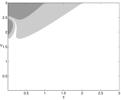
Figure 4: Attractive case. Comparison of the exact ground-state (GS) energy with the ground-state energy 9 within CPA. Different colors in the $\tau\nu$ plane are related to different value of indicator $\sigma$. White regions are characterized by an excellent agreement of the exact and the approximated GS energies. See section 5 for details.

In the attractive case, figures 1 show that the exact components (calculated numerically) are almost indistinguishable from components $X_{m}$’s obtained within the CPA and described by formula 10. The cases $N=20$ and $N=40$ that correspond to $\tau=0.02>1/J^{2}=0.01$ and $\tau=0.02>1/J^{2}=0.0025$, respectively, describe the approach from above to the lower bound of Josephson regime. In the repulsive case, figures 2 allow one to compare the exact components (calculated numerically) with components $X_{m}$’s obtained within the CPA and described by formula 29 for $\tau=0.6$ (Josephson regime), $\nu=0.8$ and $N=20,\,40$, and by formula 19 for $\tau=1.6$ (Rabi regime), $\nu=0.8$ and $N=20,\,40$. While in the first case formula 29, representing a su(2) coherent state, provides a satisfactory approximation, in the second case formula 19 exhibits a shift on the right of highest weight components $X_{m}$’s that, in addition, are smaller than the exact ones. In figure 2 (right panel) $X_{m}$’s evaluated within the CSSA better match the exact ones both qualitatively and quantitatively. When $\tau$ is increased (see figure 3), the CPA approximation (CSSA) is satisfactory even if it tends to underestimate (overestimate) exact $X_{m}$’s.

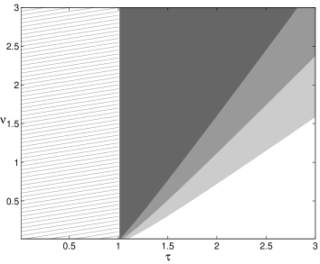
Figure 5: Repulsive case. Comparison of the exact ground-state (GS) energy with approximate GS energies. Different colors in the $\tau\nu$ plane are related to different value of indicator $\sigma$. White regions are characterized by an excellent agreement of the exact and the approximated GS energies. Details are discussed in section 5. Left panel: $\sigma$ for the GS energy 18 ($\tau>1$). Right panel: $\sigma$ for the GS energy within the CSSA. (expectation value of $H_{r}$ for the GS relevant to formula 33).

Figures 4 and 5 illustrate, through the parameter $\sigma=(E^{e}_{M}-E^{ap}_{M})/\Delta E$, the deviation of the GS energies obtained within the CPA or the CSSA from the GS energy calculated numerically. Energies $E^{e}_{M}$, $E^{ap}_{M}$, and $\Delta E$ are the exact GS energy, the approximated GS energy and the energy range defined as $\Delta E=E^{e}_{max}-E^{e}_{M}$, respectively. $E^{e}_{max}$ is the exact maximum energy. White, light grey, and dark grey colors identify the regions in the $\tau\,\nu$ plane where $\sigma<0.001$, $0.001<\sigma<0.01$ and $0.01<\sigma<0.1$, respectively. In figure 4, describing the attractive case, $E^{ap}_{M}$ is given by formula 9. $E^{ap}_{M}$ well approximates the exact GS energy in the large (white) region in the $\tau\,\nu$ plane. The repulsive case is considered in figure 5. In the left panel, $E^{ap}_{M}$ given by formula 18 is shown to well approximate the exact GS energy in a rather restricted region in the $\tau\,\nu$ plane. On the contrary, right panel shows that evaluating $E^{ap}_{M}$ based on ground-state 33 within the CSSA provides the best approximation ($\sigma<0.001$) almost everywhere. Concluding, except for the repulsive Josephson regime, where the CPA is not satisfactory, both the CPA and the CSSA provide a satisfactory approximation. The CPA is particularly good in the attractive-boson case. Among the many applications to bosonic-well systems currently studied, such approaches seem quite appropriate for studying the low-energy spectrum of the three-well boson systems where the complexity of the energy-level structure mirrors the dynamical instabilities of the chaotic three-well classical dynamics [23]. The study of similar aspects in the three-AM mode rotational fluid outlined in [3] is currently in progress.

Appendix A Classical energy minima

The classical version of the attractive model 3 displays a dynamics characterized by four (two) fixed points if $1\gg\tau$ ($\tau\gg 1$). This can be seen by considering the relevant motion equations

$${\dot{J}}_{1}=(\Delta-2|g|J_{3})J_{2},\quad{\dot{J}}_{3}=-2V_{0}J_{2},\quad{\dot{J}}_{2}=2(|g|J_{1}+V_{0})J_{3}-\Delta J_{1},\quad$$ (34)

equipped with the motion constant $J^{2}=J_{3}^{2}+J_{2}^{2}+J_{1}^{2}$, that entail the fixed-point equations $J_{2}=0$, $2|g|J_{3}J_{1}+2V_{0}J_{3}-\Delta J_{1}=0$, with the constraint $J^{2}=J_{3}^{2}+J_{1}^{2}$. Their exact solution involves a fourth-order equation in $J_{3}$, except for $\Delta=0$ when the possible solutions are either $J_{1}=-V_{0}/|g|=-J\tau$ or $J_{3}=0$. In the general case $\Delta\neq 0$, if $1\gg\tau$ and $J|g|>\Delta>0$ (namely, for $\Delta$ sufficiently small), the searched solutions are such that either $J_{3}\simeq\pm J$, $J\gg|J_{1}|$, or

$$J_{1}\simeq\pm J,\quad J\gg J_{3}>0\,.$$ (35)

This feature can be proved explicitly. Particularly, the second pair of solution is obtained by implementing the approximation $J_{1}=s{\sqrt{J^{2}-J_{3}^{2}}}$ $\simeq sJ(1-J_{3}^{2}/2J^{2})$, $s=\pm 1$. Neglecting the third order terms in $J_{3}/J$, the second fixed-point equation becomes $({\Delta}/{2J})J_{3}^{2}+2J|g|(1+s\tau)J_{3}-J\Delta=0$, whose roots are found to be $J_{3}=2J\sigma^{-1}_{s}[-1\pm{\sqrt{1+\sigma_{s}^{2}/2}}]$ with $\sigma_{s}=\Delta/[J|g|(1+s\tau)]$. While the negative root must be discarded because it entails $|J_{3}|>J$, the positive root –this can be shown to describe both a minimum ($s=+1$) and a saddle point ($s=-1$)– can be approximated as

$$J_{3}\simeq\frac{J\tau\Delta}{2V_{0}(1+s\tau)},$$ (36)

if $\delta=\Delta/|g|<J$. When $\tau>1$ (and thus for $\tau\gg 1$) the choices $s=-1,\,+1$ are related to a maximum and a minimum, respectively. Notice that the previous formula giving the $J_{3}$ coordinate is well defined for the minimum ($s=+1$) also when $\tau\gg 1$.

Let us consider now the (classical) repulsive model 4. The corresponding Hamiltonian equations read

$${\dot{J}}_{1}=(\Delta+2|g|J_{3})J_{2},\quad{\dot{J}}_{3}=-2V_{0}J_{2},\quad{\dot{J}}_{2}=2(V_{0}-|g|J_{1})J_{3}-\Delta J_{1},\quad$$ (37)

and exhibit once more the motion constant $J^{2}=J_{1}^{2}++J_{2}^{2}+J_{3}^{2}$. For $\Delta=0$ and $\tau>1$, the energy minimum is easily shown to correspond to $J_{1}=J$, $J_{2}=J_{3}=0$. Thus a generic state near the minumun is such that

$$J_{1}\simeq J,\quad|J_{2}|,\,|J_{3}|\ll J\,.$$ (38)

If $\Delta\neq 0$, provided $\Delta/J|g|$ is sufficiently small, this statement is certainly valid for $1\ll\tau=V_{0}/J|g|$ (Rabi regime). In fact, by setting $J_{1}={\sqrt{J^{2}-J_{3}^{2}}}$ $\simeq J(1-J_{3}^{2}/2J^{2})$ and neglecting the third order terms in $J_{3}/J$ in the fixed-point equation $0=2(V_{0}-|g|J_{1})J_{3}-\Delta J_{1}$, one finds $({\delta}/{2J})J_{3}^{2}+2J(\tau-1)J_{3}-\delta J=0$, whose roots are found to be $J_{3}=2J\alpha^{-1}[-1\pm{\sqrt{1+\alpha^{2}/2}}]$, with $\alpha=\Delta/[J|g|(\tau-1)]$. Discarding the negative root which entails $|J_{3}|>J$, the positive root can be approximated as

$$J_{3}\simeq\frac{\Delta}{2|g|(\tau-1)}=\frac{J\tau\Delta}{2V_{0}(\tau-1)},$$ (39)

if $\Delta/J|g|\ll\tau-1$. In the Rabi regime where $1\ll\tau\simeq\tau-1$ such condition reduces to $\Delta\ll V_{0}$. In the Fock/Josephson regimes, where $\tau<1$, the two configurations $J_{1}=\tau J$, $J_{3}=\pm J{\sqrt{1-\tau^{2}}}$ are found to minimize the energy if $\Delta=0$. This suggests that, even with $\Delta\neq 0$, low-energy states are such that

$$J_{3}\simeq\pm J,\quad|J_{2}|,\quad|J_{1}|\ll J\,.$$ (40)

To obtain the energy-minimum configurations, in addition to $J_{2}=0$, we consider the second fixed-point equation under the approximation $J_{3}=s{\sqrt{J^{2}-J_{1}^{2}}}\simeq sJ(1-J_{1}^{2}/2J^{2})$ with $s=\pm 1$. Neglecting the third order terms in $J_{1}/J$, the latter entails $0=({V_{0}}/{J})J_{1}^{2}+(2|g|J-s\Delta)J_{1}-2V_{0}J$, which supply, with $s=+1$, two minimum-energy configurations ($\delta=\Delta/|g|$)

$$J_{1}\simeq\frac{\tau J}{1+s\delta/2J},\quad J_{3}=sJ{\sqrt{1-(J_{1}/J)^{2}}}\simeq sJ\Bigl{[}1-\frac{2J^{2}\tau^{2}}{(2J+s\delta)^{2}}\Bigr{]}\,.$$ (41)

These reproduce correctly the formula of the case $\Delta=0$.

References

- [1] Rokhsar D S, preprint cond-mat/9812260
- [2] Leggett A J 2001 Rev. Mod. Physics 73 307
- [3] Ueda M and Leggett A J 1999 Phys. Rev. Lett. 8 83
- [4] Kanamoto R, Saito H, and Ueda M 2003 Phys. Rev. A 68 043619
- [5] Kanamoto R, Saito H, and Ueda M 2005 Phys. Rev. Lett. 94 090404
- [6] Milburn G J, Corney J, Wright E M and Walls D F 1997 Phys. Rev. A 55 4318
- [7] Steel M J and Collett M J 1998 Phys. Rev. A 57 2920
- [8] Spekkens R W and Sipe J E 1999 Phys. Rev. A 59 3868
- [9] Menotti C, Anglin R, Cirac J I, and Zoller P 2001 Phys. Rev. A 63 023601
- [10] Mahmud K W, Perry H and Reinhardt W P 2003 J. Phys. B: At. Mol. Opt. Phys. 36 L265
- [11] Franzosi R, Penna V and Zecchina R 2000 Int. J. Mod. Phys. B 14 943
- [12] Benet L, Jung C and Leyvraz F 2003 J. Phys. A: Math. Gen. 36 L217
- [13] Tonel A P, Links J and Foerster A cond-mat/0412214
- [14] Solomon A I 1971 J. Math. Phys. 12 390
- [15] Solomon A I, Feng Y, and Penna V 2001 Phys. Rev. B 60 3044
- [16] Kostrun M, 2004 Phys. Rev. A 70 012105
- [17] Inönü E and Wigner E P 1953 Proc. Nat. Acad. Sci. (US) 39 510
- [18] Rowe D J and Thiamova G, The many relationships between the IBM and the Bhor model to appear on Nuclear Physics A, 2005
-
[19]
Gilmore R 1974 Lie algebras lie groups and some of their applications
(Wiley, New York)
Amico L 2000 Mod. Phys. Lett. B 14 759 - [20] Franzosi R, Penna V 2001 Phys. Rev. A 63 043609
- [21] An explicit calculation gives , with . This term certainly vanishes being and . Since and then very rapidly due to the factor .
- [22] Zhang W M, Feng D H, and Gilmore R, Rev. Mod. Phys. 1990 Rev. Mod. Phys. 62, 867
-
[23]
Buonsante P, Franzosi R and Penna V
2003 Phys. Rev. Lett. 90, 050404
Pando C L, Doedel E J 2005 Phys. Rev. E 71, 056201