Renormalization group approach to multiscale modelling in materials science

Abstract

Dendritic growth, and the formation of material microstructure in general, necessarily involves a wide range of length scales from the atomic up to sample dimensions. The phase field approach of Langer, enhanced by optimal asymptotic methods and adaptive mesh refinement, copes with this range of scales, and provides an effective way to move phase boundaries. However, it fails to preserve memory of the underlying crystallographic anisotropy, and thus is ill-suited for problems involving defects or elasticity. The phase field crystal (PFC) equation— a conserving analogue of the Hohenberg-Swift equation —is a phase field equation with periodic solutions that represent the atomic density. It can natively model elasticity, the formation of solid phases, and accurately reproduces the nonequilibrium dynamics of phase transitions in real materials. However, the PFC models matter at the atomic scale, rendering it unsuitable for coping with the range of length scales in problems of serious interest. Here, we show that a computationally-efficient multiscale approach to the PFC can be developed systematically by using the renormalization group or equivalent techniques to derive appropriate coarse-grained coupled phase and amplitude equations, which are suitable for solution by adaptive mesh refinement algorithms.

I Introduction

During the last thirty years or so, the field of computational materials science has emerged as a flourishing sub-discipline of condensed matter physics. It is now relatively straightforward to compute realistic-looking materials microstructures for a variety of processing conditions, and, with enough computer power, to begin to make quantitative predictions about phase diagrams, morphological phase diagrams, growth rates and other probes of the kinetics of phase transitions. But this was not so, nor even obviously within the realms of possibility, during the 1970’s when Jim Langer, Pierre Hohenberg and others initiated studies of phase transitions kinetics and instabilities in spatially-extended systems, whose fruitful union in the 1980’s gave birth to the field of pattern formation as practiced today. In those early days, the key problems were to understand the nature of the instabilities around uniform or similarity solution states, and to capture correctly the intricate non-local and retarded feedback between interface dynamics and the (typically) diffusion fields around them. To paraphrase John Archibald Wheeler’s epigram on general relativity: solidification fronts tell heat how to flow; heat tells solidification fronts how to move.

Following a variety of innovations from Langer and collaborators, especially the introduction of phase field modelsLanger (1986); Collins and Levine (1985), and their practical implementation with improved asymptoticsKarma and Rappel (1998) and adaptive mesh refinementProvatas et al. (1998), these difficulties are largely resolved, certainly in principle, and to a significant extent in practiceWarren et al. (2002). Three dimensional structures, including fluid flow effects, can now be simulated on desktop computersJeong et al. (2001, 2003). The key conceptual difficulty that remains as a challenge to this day is the huge range of length and time scales encountered in pattern formation processes. For example, in solidification, one encounters the capillary length on the scale of $10^{-8}m$ and the dendrite tip radius on a scale ranging from tens of microns to millimetres, depending on the undercooling. The latent heat around a solidification front extends to a distance known as the diffusion length, which can be $10^{-4}m$ or larger; and finally, in a real processing experiment, there will be the system size itself, many orders of magnitude larger still.

The problem of “bridging the length and time scales” between atomic and sample dimensions is the focus of the present article. Despite much activity to address the scale-up problemPhillips (2001); Vvedensky (2004), including quasi-continuum methodsTadmor et al. (1996); Shenoy et al. (1998); Knap and Ortiz (2001); Miller and Tadmor (2002), the heterogeneous multiscale methodE et al. (2003); E and Huang (2001), multi-scale molecular dynamicsRudd and Broughton (1998); Broughton et al. (1998); Denniston and Robbins (2004); Curtarolo and Ceder (2002) and multigrid variantsFish and Chen (2004), most existing work is currently limited to crystalline materials with a few isolated defectsE and Li (2004). We mention as an exception a promising approachWarren et al. (2003) based on the phase field approach, due originally to Langer (but not published for many years)Langer (1986).

The approach advocated here introduces the atomic level of description into phase field approaches using a recently developed formalism known as the phase field crystal (PFC)Elder et al. (2002); Elder and Grant (2004). The PFC describes atom crystalline structure as a periodic density wave, and posits a natural equation of motion for the density field. Having the character of a continuum partial differential equation, it can be coarse-grained using renormalization group (RG)Goldenfeld et al. (1990); Goldenfeld (1992) and related methods (see, e.g. Bowman and Newell (1998)), developed for the quite different problem of analyzing hydrodynamic instabilitiesCross and Hohenberg (1993) in spatially-extended dynamical systemsChen et al. (1996); Graham (1996); Nozaki et al. (2000); Sasa (1997); Shiwa (2000); Cross and Newell (1984); Passot and Newell (1994); Newell et al. (1993). The coarse-grained counterparts of the density field are its amplitude and phase, for which we derive equations of motion. Once known, the density field can then be reconstructed. In this article, we sketch the derivation of effective equations at the mesoscale, and show that the numerical solution of the renormalization group equations generates solutions that are virtually indistinguishable from brute force solutions of the PFC equations of motion.

A further aspect of our work is that computational efficiency is in practice best achieved by using adaptive mesh refinement. The basic idea is that for any field whose spatial variation is essentially uniform everywhere, with localized regions of rapid variation, it makes no sense to use a uniform mesh in numerical calculations. A coarse mesh can be used in places where the field is spatially uniform, and a coarser one is used in the transition zones. In the context of phase field models, we have developed techniques to implement these ideas in an efficient manner, and demonstrated that the computational complexity of this sort of algorithm scales not with the system’s volume, but with the surface area of solidification front (transition zones)—a considerable saving for large systemsProvatas et al. (1998). The renormalization group equations derived below have solutions with the desired character: thus we intend in future work to develop adaptive mesh refinement codes for solving these equations. This topic is briefly discussed at the end of this article.

II The Phase Field Crystal Model

The phase field crystal model for a single component system describes the space-time behavior of the density $\rho(\vec{x},t)$ and is capableElder et al. (2002); Elder and Grant (2004) of capturing realistic aspects of materials dynamics, including grain growth, ductile fracture, epitaxial growth, solidification processes, and reconstructive phase transitions. By construction, the stationary states of $\rho(\vec{x})$ are periodic, and distortions of the density field by external perturbations applied to boundaries or by defects, for example, result in a raising of the free energy in accord with Hooke’s law, with higher order terms representing non-linear elasticity. This feature makes the PFC an ideal tool with which to explore nanoscale strain effects and their influence upscale to the continuum.

Let $F\{\rho\}$ denote the coarse-grained free energy functional whose minima correspond to the equilibrium (lattice) state of a $d$-dimensional system, and whose corresponding chemical potential gradient drives the dynamics of $\rho$. For single component, two-dimensional systems with a hexagonal lattice state, the appropriate form of $F$ is that originally due to BrazovskiiBrazovskii (1975):

$$F\{\rho({\bf x})\}=\int d^{d}\vec{x}\left[\rho\left(\alpha\Delta T+\lambda\left(q_{o}^{2}+\nabla^{2}\right)^{2}\right)\rho/2+u\rho^{4}/4\right]$$ (1)

where $\alpha$, $\lambda$, $q_{o}$ and $u$ can be related to material propertiesElder et al. (2002); Elder and Grant (2004), and $\Delta T$ denotes the temperature difference from some reference high temperature. For convenience it is useful to rewrite this free energy in dimensionless units, i.e., $\vec{x}\equiv\vec{r}q_{o}$, $\psi\equiv\rho\sqrt{u/\lambda q_{o}^{4}}$, $r\equiv a\Delta T/\lambda q_{o}^{4}$ and $F\rightarrow Fu/\lambda^{2}q_{o}^{8-d}$. We also use dimensionless time units $t$, related to the physical time $\tilde{t}$ in terms of the phenomenological mobility $\Gamma$ by $t\equiv\Gamma\lambda q_{o}^{6}\tilde{t}$. In these units, the equation of continuity for the density becomes

$$\partial\psi/\partial t=\nabla^{2}\left(\left[r+(1+\nabla^{2})^{2}\right]\psi+\psi^{3}\right)+\zeta.$$ (2)

The conserved Gaussian noise, required by the fluctuation-dissipation theorem to satisfy $\langle\zeta(\vec{r}_{1},t_{1})\zeta(\vec{r}_{2},\tau_{2})\rangle=-{\cal E}\nabla^{2}\delta(\vec{r}_{1}-\vec{r}_{2})\delta(\tau_{1}-\tau_{2})$ with ${\cal E}\equiv uk_{B}Tq_{o}^{d-4}/\lambda^{2}$, will not generally be important for describing phase transition kinetics, and so will henceforth be neglected here.

Elder and GrantElder and Grant (2004) have studied the mean field phase diagram of the PFC equation (2) in the one mode approximation, that is valid in the limit of small $r$, and represented in the plane of dimensionless temperature, $r$, and dimensionless average density, $\bar{\psi}$. There are three possible equilibrium solutions: a ‘liquid’, $\psi_{C}=\bar{\psi}$, a two-dimensional ‘crystal’ with triangular symmetry, $\psi_{T}=A_{T}\left(\cos(q_{T}x)\cos(q_{T}y/\sqrt{3})-\cos(2q_{T}y/\sqrt{(}3))/2\right)+\bar{\psi}$, and a smectic phase which will be ignored for present purposes. The triangular lattice can exhibit defect structures during the relaxation to equilibrium, thus capturing the kinetics of phase transformations.

III Coarse-graining of the phase field crystal equations

The dynamics of the slowly-varying amplitude and phase describes fluctuations about a given set of lattice vectors, but must be covariant with respect to rotations of those lattice vectors, so that we can properly describe polycrystalline materials with arbitrarily oriented grains. A similar situation arises in describing amplitude and phase variations of convection rolls, and in the context of the model Swift-Hohenberg Swift and Hohenberg (1977) equations, the form of the governing equations was originally proposed by Gunaratne et al. Gunaratne et al. (1994), and derived systematically from the RG formalism of Chen et al.Chen et al. (1996) by GrahamGraham (1996) (see also ref. Nozaki et al. (2000)).

The details of the corresponding calculations for the PFC will be given elsewhere, but the results can be quickly obtained by considering the linearized equation governing small variations $\widetilde{\psi}$ about the constant solution $\bar{\psi}$:

$$\frac{\partial\widetilde{\psi}}{\partial t}=\nabla^{2}\left[\left\{r+(1+\nabla^{2})^{2}\right\}+3\bar{\psi}^{2}\right]\widetilde{\psi}$$ (3)

We consider a one-mode triangular perturbation with wavenumber $q_{t}$, given by $\widetilde{\psi}=\exp(\omega t)\left[\cos(q_{t}x)\cos(q_{t}y/\sqrt{3})-\cos(2q_{t}y/\sqrt{3})/2\right]$. Substitution into (3) yields the following dispersion relation:

$$\omega=-\frac{4}{3}q_{t}^{2}\left[r+3\bar{\psi}^{2}+\left(1-\frac{4}{3}q_{t}^{2}\right)^{2}\right].$$ (4)

The fastest growing mode has $q_{t}=\pm\sqrt{3}/2$ for this perturbation, which, as was shown by Elder and GrantElder and Grant (2004) working in the one-mode approximation, is the mode which minimizes the free energy functional $\mathcal{F}[\rho]$. Thus, the uniform phase becomes unstable to hexagonal perturbations when $|\bar{\psi}|<\sqrt{-r/3}$.

The triangular phase solution can be written in more general form as

$$\psi({\vec{x}})=\sum_{j}A_{j}(t)\exp(i{\vec{k_{\it{j}}}\cdot\vec{x}})+\bar{\psi},$$ (5)

where ${\vec{k_{1}}}=k_{0}({-\vec{\mbox{i}}\sqrt{3}/2}-{\vec{\mbox{j}}/2})$, ${\vec{k_{2}}}=k_{0}{{\vec{\mbox{j}}}}$ and ${\vec{k_{3}}}=k_{0}({\vec{\mbox{i}}\sqrt{3}/2}-{\vec{\mbox{j}}/2})$ are the reciprocal lattice vectors, $\vec{\mbox{i}}$ and $\vec{\mbox{j}}$ are unit vectors in the $x$- and $y$-directions, $k_{0}$ is given by $q_{t}$ and $A_{j}(t)\equiv A_{j}^{0}\exp(\omega_{j}t)$.

Substituting into (3) and applying orthogonality conditions, we readily obtain

$$\omega_{j}=-|{\vec{k_{\it{j}}}}|^{2}\left[-\Gamma+\left\{1-|{\vec{k_{\it{j}}}}|^{2}\right\}^{2}\right],$$ (6)

where $\Gamma\equiv-(r+3\bar{\psi}^{2})$, and we have transformed to units where $k_{0}=1$. In order to obtain the spatial component of the amplitude equation we study the effect of applying small spatial modulations to the amplitude, i.e.

$$A_{j}(t)\longmapsto A_{j}(x,y,t)=A_{j}^{0}\exp(\omega_{j}({\vec{Q}})t)\exp(i{\vec{Q}\cdot\vec{x}}),$$ (7)

where ${\vec{Q}}=Q_{x}\;{\vec{i}}+Q_{y}\;{\vec{j}}$ is the perturbation vector. The exponent controlling the growth rate along each lattice basis vector is given by

$$\omega_{j}({\vec{Q}})=|{\vec{Q}}+{\vec{k_{\it{j}}}}|^{2}\left[\Gamma-\left\{1-|{\vec{Q}}+{\vec{k_{\it{j}}}}|^{2}\right\}^{2}\right].$$ (8)

Replacing Fourier variables by gradient operators, we obtain

$$|{\vec{Q}}+{\vec{k_{\it{j}}}}|^{2}\equiv-{\vec{\nabla}}^{2}-2i{\vec{k_{\it{j}}}}\cdot{\vec{\nabla}}+1.$$ (9)

Putting together Eq. (8) and Eq. (9), we find that space-time amplitude variations along each basis are governed by:

$$\frac{\partial A_{j}}{\partial t}=\left[1-{\vec{\nabla}}^{2}-2i{\vec{k_{\it{j}}}}\cdot{\vec{\nabla}}\right]\left[\Gamma-\left\{{\vec{\nabla}}^{2}+2i{\vec{k_{\it{j}}}}\cdot{\vec{\nabla}}\right\}^{2}\right]A_{j}.$$ (10)

The manifestly rotationally covariant operator on the right hand side of (10) will be denoted by $\widetilde{\mathcal{L}}_{j}$.

The non-linear component of the amplitude equation is obtained by renormalizing the secular terms in the perturbation series about the periodic stateChen et al. (1996); Graham (1996); Nozaki et al. (2000). Expanding about the one-mode triangular phase solution, scaling $\psi$ by the factor $\sqrt{-r}$, and renaming the new variable $\psi$,yields the PFC equation in the form

$$\frac{\partial\psi}{\partial t}=\vec{{\nabla}}^{2}(1+\vec{{\nabla}}^{2})^{2}\psi+\epsilon\vec{{\nabla}}^{2}(\psi^{3}-\psi),$$ (11)

where $\epsilon\equiv-r$. Expanding $\psi$ as $\psi=\psi_{0}+\epsilon\psi_{1}+\epsilon^{2}\psi_{2}+\mathcal{O}(\epsilon^{3})$ and substituting in Eq. (11), using Eq. (5) for $\psi_{0}$, we obtain at $\mathcal{O}(\epsilon)$,

$$\frac{\partial\psi_{1}}{\partial t}-\vec{{\nabla}}^{2}(1+\vec{{\nabla}}^{2})^{2}\psi_{1}=\vec{{\nabla}}^{2}(\psi_{0}^{3}-\psi_{0}).$$ (12)

The secular terms on the right hand side can be identified from the expansion

$$\vec{{\nabla}}^{2}(\psi_{0}^{3}-\psi_{0})=(1-3\bar{\psi}^{2})\sum_{j}A_{j}\exp(i{\vec{k_{\it{j}}}\cdot\vec{x}})$$

$$-3A_{1}\left(|A_{1}|^{2}+2|A_{2}|^{2}+2|A_{3}|^{2}\right)\exp(i{\vec{k}_{1}\cdot\vec{x}})$$

$$-3A_{2}\left(2|A_{1}|^{2}+|A_{2}|^{2}+2|A_{3}|^{2}\right)\exp(i{\vec{k}_{2}\cdot\vec{x}})$$

$$-3A_{3}\left(2|A_{1}|^{2}+2|A_{2}|^{2}+|A_{3}|^{2}\right)\exp(i{\vec{k}_{3}\cdot\vec{x}})$$

$$-6A_{2}^{*}A_{3}^{*}\bar{\psi}\exp(i{\vec{k}_{1}\cdot\vec{x}})-6A_{1}^{*}A_{3}^{*}\bar{\psi}\exp(i{\vec{k}_{2}\cdot\vec{x}})$$

$$-6A_{1}^{*}A_{2}^{*}\bar{\psi}\exp(i{\vec{k}_{3}\cdot\vec{x}}).$$ (13)

Aligning the secular terms in Eq. (III) along each basis, and scaling back to the original variables, we obtain the amplitude equations as

$$\frac{\partial A_{1}}{\partial t}=\widetilde{\mathcal{L}}_{1}A-3A_{1}\left(|A_{1}|^{2}+2|A_{2}|^{2}+2|A_{3}|^{2}\right)-6\bar{\psi}A_{2}^{*}A_{3}^{*}.$$ (14)

together with the appropriate permutations for $A_{2}$ and $A_{3}$.

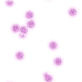
(a) $t=56.04$

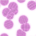
(b) $t=184.04$

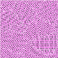
(c) $t=720.04$

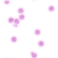
(d) $t=56.04$

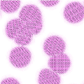
(e) $t=184.04$

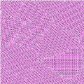
(f) $t=720.04$

Figure 1: Comparison of heterogeneous nucleation and growth in the PFC equation Eq. (2) (panels (a)-(c)) and its RG-generated mesoscale counterpart Eq. (14) (panels (d)-(f)). The order parameter is shown at the times indicated starting from the same initial condition with $\bar{\psi}=0.285$ and $r=-0.25$.

Fig. (1) shows the time evolution for the nucleation and growth of a two-dimensional film, calculated using the PFC equation and its RG-generated mesoscale counterpart. Starting from the same initial condition of randomly-oriented seeds, crystalline domains grow, colliding to form a polycrystalline microstructure. The solutions from the two different computational algorithms are essentially indistinguishable. Without the PFC formulation, it would not have been possible to capture successfully the formation of a polycrystalline material, with grain boundaries and other defects. We conclude that it is indeed possible to compute large scale microstructure from effective equations at the mesoscale.

IV Computational efficiency

In order for our scheme to be computationally efficient, we need to establish that the solutions for the fundamental mesoscale variables are indeed slowly varying. In Fig. (2) are shown the amplitude and phase gradient of one of the components during the computation of the two-dimensional grain growth. It is evident that the variables are indeed essentially uniform, except near the edges of the grains.

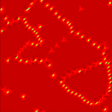
(a)

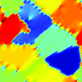
(b)

Figure 2: Color map of the spatial variation of the amplitude (a) and phase gradient (b) of the solution displayed in Fig. (1) at time $t=720.04$.

In order to exploit this property computationally, we need to work with a formulation which is independent of the particular orientation of our reference directions. To this end, we reformulate the RG-PFC equations for the complex amplitudes $A_{j}$ etc. in terms of their real amplitude and phase variables, denoted by $\Psi_{j}>0$ and $\Phi_{j}$. Expanding out the terms in Eq. (14), and equating real and imaginary parts, we obtain equations of motion for $\Psi_{j}$ and $\nabla\Phi_{j}$ which can readily be solved by adaptive mesh refinement, to be reported elsewhere. This formulation is also important in treating the beats that can arise if the crystallographic axes of a grain are not collinear to the basis axes used in the numerical solution. Such beats can be dealt with by either adaptive mesh refinement or the polar coordinate formulation, and will be discussed in detail elsewhere. As we have previously shownProvatas et al. (1998), adaptive mesh refinement algorithms scale optimally, with the number of computations being proportional to the number of mesh points at the finest scale, i.e. to the grain boundary length (two dimensions) or surface area (three dimensions).

In summary, we have shown that multiscale modeling of complex polycrystalline materials microstructure is possible using a combination of continuum modeling at the nanoscale using the PFC model, RG and related techniques from spatially-extended dynamical systems theory. The PFC model can be extended to include three dimensions, multi-component systems, thermal fields and realistic atomic correlations. Our analysis is ideally-suited for efficient adaptive mesh refinement, thus enabling realistic modeling of large-scale materials processing and behavior.