Classical Region of a Trapped Bose Gas

Abstract

The classical region of a Bose gas consists of all single-particle modes that have a high average occupation and are well-described by a classical field. Highly-occupied modes only occur in massive Bose gases at ultra-cold temperatures, in contrast to the photon case where there are highly-occupied modes at all temperatures. For the Bose gas the number of these modes is dependent on the temperature, the total number of particles and their interaction strength. In this paper we characterize the classical region of a harmonically trapped Bose gas over a wide parameter regime. We use a Hartree-Fock approach to account for the effects of interactions, which we observe to significantly change the classical region as compared to the idealized case. We compare our results to full classical field calculations and show that the Hartree-Fock approach provides a qualitatively accurate description of classical region for the interacting gas.

I Introduction

There has been much recent work on using the classical field approximation to model Bose-Einstein condensates at zero and finite temperatures Davis et al. (2002); Davis and Morgan (2003); Davis and Blakie (2005, 2006); Simula and Blakie (2006); Gardiner et al. (2002); Gardiner and Davis (2003); Gòral et al. (2001); Davis et al. (2001a, b); Lobo et al. (2004); Marshall et al. (1999); Norrie et al. (2005); Polkovnikov and Wang (2004); Sinatra et al. (2001, 2002); Steel et al. (1998); Bradley et al. (2005); Blakie and Davis (2005). At zero temperature a single mode of the system (the condensate) is macroscopically occupied and its evolution is well-described by the Gross-Pitaevskii equation. The classical field approximation is also suited to finite temperature regimes where many modes of the system are highly occupied (also see Svistunov and Shlyapnikov (1991)). The major advantage of classical field approaches over other methods is that interactions between the modes can be treated non-perturbatively, making the formalism suitable for non-equilibrium studies.

The purpose of this paper is to fully characterize the size and nature of the classical region for typical experimental parameters. These properties of the classical region are not a priori obvious, especially for the case of an interacting gas. Better characterization of the classical region will be useful for: (a) informing better choice of parameters for classical field simulations of finite temperature gases; and (b) demonstrating the regimes of applicability of this theory.

I.1 Historic Motivation: Blackbody Radiation

We begin by reviewing a topic of modern physics that was responsible for the quantum revolution, yet also serves as motivation for the application of the classical field approximation to quantum fields: the spectrum of radiation from a blackbody. Approximately a century ago the Rayleigh-Jeans theory of the light spectrum emitted from a blackbody was developed upon a classical field theory (i.e. Maxwell’s electromagnetic theory) in conjunction with statistical methods. The famous failure of this theory eventually led to the discovery that light is constituted of photons, and initiated the quantum revolution in physics. However, an observation of prime importance is that the Rayleigh-Jeans theory is actually extremely successful at predicting the behaviour of the blackbody spectrum for the long wavelength modes. We illustrate this point in Fig. 1(a), where the quantum and classical predictions for the spectrum are compared for a blackbody at a temperature of $T=2500$ K. The most distinctive feature of this graph is the rather alarming disagreement at small wavelengths, the so-called ultra-violet catastrophe. However at larger wavelengths, greater than $5\mu$m say, the agreement between the quantum and classical predictions becomes increasingly good. For these long wavelength modes each photon carries only a small amount of energy compared to $k_{B}T$, so that on average these modes contain a large number of photons. This high occupancy is what we will refer to as the classical limit for a field. For these modes the discreteness of the energy each photon carries is masked by the large number of other photons in the same mode and the classical theory provides a good description. We note that this is quite different from the high temperature classical limit for particles, when Bose/Fermi statistics can be approximated by Maxwell-Boltzmann statistics. The ultra-violet catastrophe occurs because the classical theory fails to describe the short wavelength modes correctly. These modes are sparingly occupied by photons and require a proper quantum treatment. In Fig. 1(b) the mean number of photons per mode is shown, and comparison with Fig. 1(a) clearly reveals that the quantum and classical theories agree well where the mean number of photons is large. In general any electromagnetic mode can be made classical by making the temperature sufficiently large as photon number is not conserved.

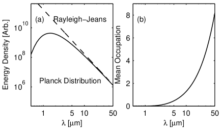
Figure 1: (a) Quantum and classical theories for the energy spectrum of a blackbody at $T=2500$ K. (b) The mean number of photons in each mode at $T=2500$ K calculated using the Planck distribution.

I.2 Classical Region of a Bose Gas

Atoms are necessarily conserved and require a chemical potential ($\mu$) in their statistical description. By expanding the Planck and Bose-Einstein distributions for high occupation $n(\epsilon)\gg 1$ we find the following requirements on the single particle energies

$$\epsilon \ll k_{B}T\qquad\rm{Planck},$$ (1)

$$\epsilon-\mu \ll k_{B}T\qquad\rm{Bose-Einstein}.$$ (2)

We note that in these limits the classical equipartition theorem holds . For the Bose gas at high temperatures (the Maxwell-Boltzmann limit) the chemical potential is large and negative

$$\mu\approx-k_{B}T\ln\left[\frac{V}{N}\left(\frac{2\pi mk_{B}T}{h^{2}}\right)^{3/2}\right],$$ (3)

where $V$ is the system volume and $N$ is the number of atoms. In contrast to the photon case, this behaviour of $\mu$ prevents the mean occupation of any individual mode from becoming large as $T$ increases.

Indeed, for a gas of atoms at temperatures above the microkelvin regime, the average occupation of the system modes is much less than unity and the particle-like behaviour of the system dominates over the wave-like behaviour. However, at temperatures approaching the condensation temperature ($T_{c}$), the chemical potential approaches the ground state energy, and many modes of the system may become highly occupied. The nature of these highly occupied modes (outside of the condensate itself) is not widely appreciated, and is the central topic we address in this paper. We refer to these modes as the constituting the classical region, for which the classical field approximation is appropriate: We can replace the quantum mode operators $\{\hat{a}_{j}\}$, satisfying the commutation relations $[\hat{a}_{i},\hat{a}_{j}^{\dagger}]=\delta_{ij}$, with the c-number amplitudes $\{c_{j}\}$. Modes outside the classical region are more sparsely occupied and are poorly described by the classical field approximation — these modes constitute the incoherent region. In this paper we characterize the classical region of a trapped Bose gas as a function of temperature and total particle number, and show that the classical field approximation should be widely applicable to current experiments.

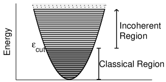
Figure 2: Schematic diagram showing the classical and incoherent regions of the single particle spectrum for a harmonically trapped Bose gas. At the energy $\epsilon_{{\rm cut}}$ the average occupation is $n_{{\rm cut}}\sim 3$ (see the text).

Schematically we show the classical and incoherent regions in Fig. 2, for the case of the harmonically trapped gas. The classical region is quantitatively defined as those single particle modes with mean occupation greater than $n_{{\rm{cut}}}$, where $n_{{\rm{cut}}}$ is the minimum occupation we require for a mode to be designated as classical. As the single particle occupation monotonically decreases with increasing energy, the boundary of the classical region occurs at an energy we define to be the cutoff energy, $\epsilon_{{\rm cut}}$. With reference to the electromagnetic case shown in Figs. 1(a)-(b), we see that an adequate condition for the classical field description to be valid is found by taking $n_{{\rm cut}}\sim 3$ (i.e. blackbody modes with a mean occupation of $\geq 3$ photons are equally well-described by the Planck and Rayleigh-Jeans distributions). We note that other authors have suggested that taking $n_{{\rm cut}}\sim 5$ to $10$ particles may be more suitable Gardiner and Davis (2003). The precise value of $n_{{\rm cut}}$ used will be unimportant for the qualitative characteristics of the classical region we investigate here.

I.3 Projected Gross-Pitaevskii Equation Formalism

In this paper we are not primarily concerned with the details of applying the classical field technique to model Bose gases, but will briefly review the formalism to establish the context and importance of the classical region. The evolution equation for the classical modes of an interacting Bose field is given by Projected Gross-Pitaevskii equation (PGPE) Davis et al. (2001b, a, 2002); Blakie and Davis (2005):

$$i\hbar\frac{\partial\Psi}{\partial t} = \left(-\frac{\hbar^{2}}{2m}\nabla^{2}+V_{{\rm trap}}(\mathbf{x})\right)\Psi+\,\mathcal{P}\bigg{\{}U_{0}|\Psi|^{2}\Psi\bigg{\}},$$ (4)

where $\Psi=\Psi(\mathbf{x},t)$ is the classical matter wave field (i.e. describes the atoms in the classical region), $V_{{\rm trap}}(\mathbf{x})$ is the external trapping potential and $U_{0}=4\pi a\hbar^{2}/m$, with $a$ the s-wave scattering length. The projector is defined as

$$\mathcal{P}\{F(\mathbf{x})\}\equiv\sum_{n\in\mathcal{C}}\varphi_{n}(\mathbf{x)}\int d^{3}\mathbf{x}^{\prime}\varphi_{n}^{*}(\mathbf{x^{\prime}})F(\mathbf{x^{\prime}}),$$ (5)

where $\varphi_{n}(\mathbf{x})$ are eigenstates of the single particle Hamiltonian $H_{{\rm sp}}=-\frac{\hbar^{2}}{2m}\nabla^{2}+V_{{\rm trap}}(\mathbf{x})$ and the summation is restricted to modes in the classical region. The action of $\mathcal{P}$ in Eq. (5) is to project the arbitrary function $F(\mathbf{x})$ into the classical region. A description of the incoherent particles will also be required for quantitative comparison with experiments and a formalism for including this into the PGPE theory has been presented in Ref. Gardiner and Davis (2003).

Previous work has shown that the PGPE will evolve randomised initial conditions to thermal equilibrium Davis et al. (2001b, 2002); Blakie and Davis (2005); Gòral et al. (2001, 2002). The equilibrium state that is reached depends on three input parameters: (i) The number of atoms in the classical region, which we refer to as $N_{{\rm below}}$; (ii) The total energy content of the classical region $E$; (iii) The cutoff energy $\epsilon_{{\rm cut}}$ determining the size of the classical region (i.e. the number of classical modes $M_{\rm{below}}$ ).

In dynamical simulations of Eq. (4), interactions cause the system to rapidly thermalize Davis et al. (2002), and subsequently (using the ergodic hypothesis) time-averaging can be used to extract equilibrium quantities. A major challenge for classical field approaches has been to determine thermodynamics quantities that are derivatives of entropy, such as temperature. This was recently overcome in Ref. Davis and Morgan (2003); Davis and Blakie (2005), using formalism initially developed by Rugh Rugh (1997). A remaining issue with using the classical field approach is that the thermodynamic parameters for the simulation (such as the temperature, and the total number of atoms in the system, i.e. including those above the cutoff) are only apparent a posteriori. The characterization of the classical region we give here should facilitate making a reasonable a priori estimate of parameters for PGPE simulations and should be of great practical benefit.

II Formalism

For the results presented in Figs. 3 and 4 we consider (bosonic) rubidium-87 in an isotropic harmonic trapping potential with single-particle energy spectrum $\epsilon=\hbar\omega(n_{x}+n_{y}+n_{z}+\frac{3}{2}),$ where $\omega=2\pi\times 100$ Hz is the harmonic trap frequency (chosen to be comparable with typical experiments). To account for interaction effects we use the semiclassical Hartree-Fock (HF) density of states

$$\rho_{\rm{HF}}(\epsilon)=\int\frac{d^{3}\mathbf{x}d^{3}\mathbf{p}}{(2\pi\hbar)^{3}}\delta\left(\epsilon-\left[\frac{p^{2}}{2m}+V_{\rm{trap}}(\mathbf{x})+2U_{0}n_{c}(\mathbf{x})\right]\right),$$ (6)

where the condensate density is given by the Thomas-Fermi approximation

$$n_{c}(\mathbf{x})=\left\{\begin{matrix}\frac{1}{U_{0}}(\mu_{\rm{TF}}-V_{\rm{trap}}(\mathbf{x})),\qquad&\mu-V_{\rm{trap}}(\mathbf{x})\geq 0,\\ 0,&\mu_{\rm{TF}}-V_{\rm{trap}}(\mathbf{x})<0,\\ \end{matrix}\right\}$$ (7)

and $\mu_{\rm{TF}}$ is the Thomas-Fermi approximation to the condensate eigenvalue (e.g. see Dalfovo et al. (1999); Bijlsma et al. (2000)). The Thomas-Fermi approximation is only valid for large condensate number, however, for small condensate numbers the density of states is largely unchanged from the ideal gas case, and so for our purposes this approximation is valid for all temperatures.

To study the statistical properties of this system at finite temperature we work in the grand canonical ensemble thermally occupying the particle states described by (6) using the Bose-Einstein distribution function

$$n_{{\rm BE}}(\epsilon)=\frac{1}{e^{\beta\epsilon}/z-1},$$ (8)

where $\beta=1/k_{B}T$ is the inverse temperature, $z=e^{\beta\mu}$ is the fugacity, and the excitation energy $\epsilon$ is measured relative to the chemical potential ($\mu_{\rm{TF}}$). To calculate the thermodynamic properties as a function of the total number of particles $N_{T}$ it is necessary to find the fugacity subject to the requirement that the mean number of particles is equal to $N_{T}$. This parameter must be adjusted carefully as the condensate number, condensate density and excitation spectrum all change with $z$.

Of interest for us is to identify the properties of the classical region, in particular the number of classical modes ($M_{\rm{below}}$) and their combined occupation ($N_{\rm{below}}$). According to Eq. (8) the energy at which the mean occupation is equal to $n_{\rm{cut}}$ is given by

$$\epsilon_{{\rm cut}}=k_{B}T\ln\left[z\left(1+\frac{1}{n_{{\rm cut}}}\right)\right],$$ (9)

Integrating the density of states (6) up to this energy we obtain the number of particle states,

$$M_{\rm{below}}=\int_{0}^{\epsilon_{\rm{cut}}}d\epsilon\,\rho_{\rm{HF}}(\epsilon),$$ (10)

which we refer to as the number of classical modes. Finally, the combined occupation of the classical modes is given by

$$N_{\rm{below}}=\int_{0}^{\epsilon_{\rm{cut}}}d\epsilon\,n_{\rm{BE}}(\epsilon)\rho_{\rm{HF}}(\epsilon).$$ (11)

III Results

III.1 Ideal Gas

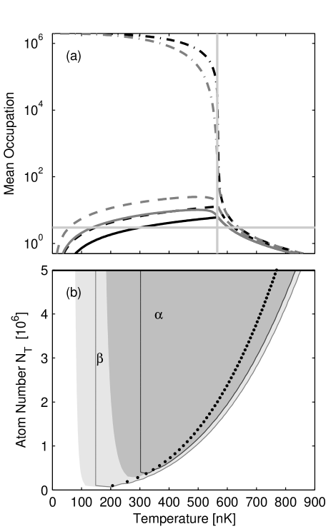
Figure 3: (a) Mean occupation of the condensate and selected excited single particle states for both ideal (black curves) and interacting (grey curves) systems of $2\times 10^{6}$ rubidium-87 atoms in a 3D 100 Hz isotropic trap. Condensate: dash-dot. $M=120^{\rm{th}}$ single particle level: solid. $M=1000^{\rm{th}}$ single particle level: dashed. The horizontal light-grey line indicates $n_{{\rm cut}}=3$ particles per mode. The vertical light-grey line marks $T_{c}$ for this system. (b) Phase diagram of the classical region. The dark shaded region labelled $\alpha$ is where the $M=1000{}^{{\rm th}}$ single particle level has a mean occupation of greater than 3 particles. The lighter shaded region labelled $\beta$ is where the $M=120{}^{{\rm th}}$ single particle level has a mean occupation of greater than 3 particles. The boundaries of these regions for the non-interacting case are shown as grey lines and $T_{c}$ is shown as with black dots.

Typical results for the mode occupations are shown in Fig. 3(a) for a system of $N_{T}=2\times 10^{6}$ atoms. Here we discuss the ideal gas results, and refrain from considering the interacting results until the next subsection.

Far above the transition temperature, $T_{c}\approx 566$ nK, the occupation of all modes is small compared to unity and there is no classical region. At $T\approx 640$ nK the occupation of several modes exceed $n_{{\rm cut}}=3$ atoms and a classical region develops in the system. At temperatures equal to, or less than $T_{c}$, the occupation of the condensate mode dominates the system, however a large number of other modes have occupations exceeding $n_{{\rm cut}}$. At temperatures near $T_{c}$ of order a thousand single particle states participate in the classical region. This can be seen from Fig. 3(a) where the where the dashed line representing the occupation of the $1000^{{\rm th}}$ single particle state is above the dotted line marking $n_{{\rm cut}}$ for a range of temperatures encompassing $T_{c}$. States of lower energy remain highly occupied over a broader temperature range (e.g. the $\epsilon=8.5\hbar\omega$ mode occupation, represented by the dash-dot line in Fig. 3(a), exceeds $n_{{\rm cut}}$ over a broader range than the $\epsilon=17.5\hbar\omega$ mode). Thus the number of modes in the classical region $M_{\rm{below}}$ varies significantly with temperature, but is largest at $T_{c}$ where the non-condensate modes have their maximum occupation.

The classical regions for two particular modes are shown in Fig. 3(b) as a function of temperature and total number of particles. In region $\alpha$ the mean occupation of the $\epsilon=17.5\hbar\omega$ state exceeds $n_{{\rm cut}}$. In the broader region $\beta$ the mean occupation of the $\epsilon=8.5\hbar\omega$ state exceeds $n_{{\rm cut}}$. The left hand edges of the regions are independent of $N_{T}$ (i.e. the boundary of the region is vertical). This is because the thermal cloud is saturated for $T<T_{c}$, and the mode occupation only depends on temperature. We can quantitatively predict the left-hand boundary by noting that below transition temperature the chemical potential is well approximated by taking it equal to the ground state energy, i.e. $\mu\approx\epsilon_{0}$, inverting the Bose-Einstein distribution function we obtain

$$T_{LH}=\frac{\epsilon-\epsilon_{0}}{k_{B}\ln(1+1/n_{{\rm cut}})},$$ (12)

independent of $N_{T}$ and in agreement with the left-hand boundaries in Fig. 3(b).

The right hand boundary occurs above $T_{c}$ where $\mu$ is different from $\epsilon_{0}$, and is seen to be dependent on $N_{T}$. We note that for large $N_{T}$ the classical region extends to temperatures considerably above $T_{c}$, indeed for the case considered in Fig. 3(b) the classical region begins $\sim 100$ nK above $T_{c}$ for $N_{T}>3\times 10^{6}$ particles.

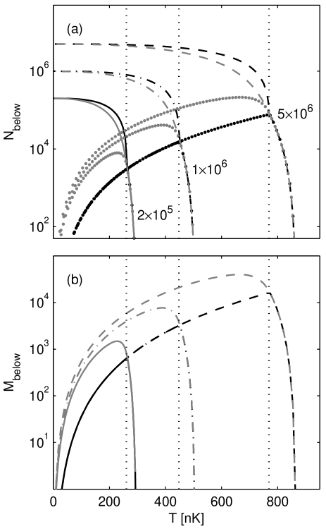
Figure 4: The classical region for rubidium-87 atoms in a 3D isotropic harmonic trap with $\omega=2\pi\times 100$ Hz. (a) The total number of atoms in modes with occupation greater than 3 ($N_{{\rm below}}$) for systems with a total of $5\times 10^{5}$ (solid line), $1\times 10^{6}$ (dash-dot line), and $5\times 10^{6}$ (dashed line) atoms. The dotted curves show the number of atoms constituting $N_{{\rm below}}$ that are not in the condensate. (b) The number of modes in the classical region $M_{{\rm below}}$ for the systems in (a). For all curves in this plot black curves are for the non-interacting case and grey curves include the effects of interactions. For reference $T_{c}$ is indicated using vertical dotted lines in each plot.

In Fig. 4 we characterise the total number of atoms ($N_{{\rm below}}$) and modes ($M_{{\rm below}}$) participating in the classical region as a function of temperature for several values of $N_{T}$. For $T<T_{c}$, $N_{{\rm below}}$ is dominated by the condensate mode and scales as $N_{{\rm{\rm below}}}\sim\{1-(T/T_{c})^{3}\}$, as can be seen for the three cases of $N_{T}$ considered in Fig. 4(a). The number of classical region particles not in the condensate is shown as the dotted curve in Fig. 4(a). We notice that up to the transition temperature this curve is independent of $N_{T}$, due to the saturated nature of the thermal cloud. Though the population of these classical non-condensate particles is much less than the condensate, for the cases considered in Fig. 4(a) we see that they may constitute up to $\leavevmode\nobreak\ \sim 10^{5}$ particles. Additionally, above $T_{c}$ there is no condensate and the classical non-condensate particles dominate the classical region.

In Fig. 4(b) we consider the behaviour of the cutoff energy. For $T<T_{c}$ the cutoff energy increases linearly with temperature, and is independent of $N_{T}$. As discussed above, for $T<T_{c}$ the chemical potential is well-approximated as the ground state energy $\mu\to\epsilon_{0}$, and we can find an explicit expression for the cutoff energy in terms of the temperature

$$\epsilon_{{\rm cut}}=k_{B}T\ln\left(1+\frac{1}{n_{{\rm cut}}}\right)+\epsilon_{0},\qquad(T\leq T_{c}),$$ (13)

(or equivalently, $M_{\rm{below}}=\epsilon_{\rm{cut}}^{3}/6(\hbar\bar{\omega})^{3}$, where $\bar{\omega}$ is the geometric mean of the harmonic trap frequencies). Reaching its maximum value at $T_{c}$, the cutoff energy decreases for $T>T_{c}$ as the classical region shrinks due to the rapid decrease in $\mu$.

III.2 Hartree-Fock Results

The results for the interacting gas, calculated using the density of states given in Eq. (6), are also shown in Figs. 3 and 4. There are many qualitative differences introduced in the interacting case. First, for the interacting system the size and number of particles in the classical regions tends to be larger than the ideal case. Second, the number of modes of the classical region ($M_{\rm{below}}$) tends to peak at temperatures below $T_{c}$ for the interacting case, whereas it peaks at $T_{c}$ for the ideal case. These effects are related and can be understood by examining the density of states (6). Due to the mean field repulsion of the condensate, the lowest energy excitations do not occupy the phase space coordinates near the origin, but for position values near the surface of the condensate. Because of the increased amount of phase space available at the surface of the condensate more low energy states are available. As the temperature increases the condensate fraction and radius both decrease, reducing this phase space enhancement. The observed maximum of $M_{\rm{below}}$ in Fig. 4(b) occurs due to the competition between increasing temperature (which tends to increase the number of accessible states) and reducing condensate radius (which reduces the number of low energy modes).

IV Comparison to PGPE

It is of interest to assess how well the ideal gas and Hartree-Fock results for the classical region describe the classical field case. Because the PGPE approach includes interactions between the excitations we expect quantitative differences with the Hartree-Fock results to arise. Our procedure for calculating equilibrium properties for the trapped Bose gas is discussed in Ref. Davis and Blakie (2006). Briefly, the PGPE system is a microcanonical system with external constants of motion (i.e. thermodynamic constraints) of $N_{below}$ and total energy $E$. Additionally, to avoid an ultraviolet divergence a restriction in the single particle modes must be made by selecting $M_{below}$. After equilibrium is found and the properties of the classical region are determined, such as mean density, temperature and chemical potential, the incoherent region can be found using a semiclassical Hartree-Fock analysis.

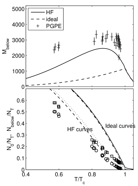
Figure 5: Comparison of classical region estimates using the methods described in this paper to the numerical PGPE results as a function of temperature. (a) Number of classical region modes for $n_{\rm{cut}}=2.8$: HF (solid), ideal gas (dashed), PGPE solution (+), indicating estimated error bars vertically. (b) Classical region fractional population: HF (dotted), ideal gas (solid), PGPE solution (square). Condensate fraction: HF (dashed), ideal gas (dash-dot), PGPE solution (circle). Harmonic trap with oscillation frequencies $\{f_{x},f_{y},f_{z}\}=\{1,1,\sqrt{8}\}\times 40$ Hz containing approximately $3\times 10^{5}$ ⁸⁷Rb atoms.

The results of this study are shown in Fig. 5. These confirm that the HF predictions are qualitatively in much better agreement with the PGPE theory than the ideal case. We note the following points:

1. Temperature in Fig. 5 has been scaled in terms of the ideal transition temperature. The PGPE exhibits the condensation transition at $T/T_{c}<1$ due to the downward shifts in critical temperature arising from finite size and interaction effects (neither of these effects are in the ideal or HF results).

2. The PGPE results suggest that number of classical modes, $M_{\rm{below}}$, does not increase up to the critical point (as predicted by the ideal result), and are consistent with the HF prediction of a maximum value occurring for $T<T_{c}$.

3. The number of classical region modes is considerably larger than predicted by the HF method. However, as the total number of modes $M_{\rm{below}}$ is proportional to $\epsilon_{cut}^{3}$ for the ideal gas then the increase in $\epsilon_{cut}$ is not as significant.

V Conclusions and Outlook

We have characterized the classical region, containing modes with occupations higher than $n_{{\rm cut}}\sim 3$, as a function of the total number of particles and temperature for a harmonically trapped Bose gas. To do this we have examined the number of modes and number of particles in the classical region, and the behaviour of the energy cutoff.

For the ideal case we have shown that for $T>T_{c}$ the cutoff energy is dependent on the total number of atoms in the system and the temperature, whereas for $T<T_{c}$ the cutoff energy increases linearly with temperature and is independent of $N_{T}$.

We have studied interaction effects using a Hartree-Fock approach which we have compared with full PGPE simulations. Our results show that interactions have a considerable effect on the classical region, and appear to make the size of the classical region much greater than predicted by an ideal gas analysis.

In general we have demonstrated that for systems with of order a million particles the classical region may consist of thousands of single particles states and extend to temperatures of order $100$ nK above $T_{c}$. Overall these results demonstrate that the PGPE technique has a wide range of applicability to trapped Bose gases and should facilitate better parameter estimation necessary for effectively applying the PGPE formalism to model experiments.